


ABSTRACT
The interaction of gas-rich galaxies with the intracluster medium (ICM) of galaxy clusters has a remarkable impact on their evolution, mainly due to the gas loss associated with this process. In this work, we use an idealized, high-resolution simulation of a Virgo-like cluster, run with ramses and with dynamics reproducing that of a zoom cosmological simulation, to investigate the interaction of infalling galaxies with the ICM. We find that the tails of ram pressure stripped galaxies give rise to a population of up to more than a hundred clumps of molecular gas lurking in the cluster. The number count of those clumps varies a lot overtime – they are preferably generated when a large galaxy crosses the cluster (M200c > 1012 M⊙), and their lifetime (≲ 300 Myr) is small compared to the age of the cluster. We compute the intracluster luminosity associated with the star formation that takes place within those clumps, finding that the stars formed in all of the galaxy tails combined amount to an irrelevant contribution to the intracluster light. Surprisingly, we also find in our simulation that the ICM gas significantly changes the composition of the gaseous discs of the galaxies: after crossing the cluster once, typically 20 per cent of the cold gas still in those discs comes from the ICM.
1 INTRODUCTION
The environment of a galaxy is an important driver for its evolution across a range of scales. One recurrent scenario is that of a small satellite orbiting a large halo and being affected by it, which can be a dwarf galaxy orbiting a massive one or a galaxy orbiting a galaxy cluster (see Gunn & Gott 1972; Mateo 1998). These interactions give rise to a universal dependence of galaxy properties on local density (Kauffmann et al. 2004; Wetzel et al. 2013), suggesting that, in a model of galaxy evolution, the environment must be taken into account in order to explain the observed properties of galaxies in the Universe.
In the case of galaxy clusters, orbiting galaxies suffer the influence of the diffuse and hot gaseous medium of these structures, known as the intracluster medium (ICM). As described in Gunn & Gott (1972), the ram pressure exerted by the ICM can remove gas from the galaxies, in a process called ram pressure stripping. This process has been extensively reported in observations and is often associated with remarkable ‘jellyfish’ morphologies, in which the galaxies feature a tail of stars and stripped gas organized in filaments and clumps (Ebeling, Stephenson & Edge 2014; McPartland et al. 2016; Poggianti et al. 2016). For a gas-rich disc galaxy, the ram pressure strips first the less gravitationally bound outskirts of its gaseous disc, causing it to feature a truncated H i disc after a partial stripping event, such as has been observed in several Virgo (Cayatte et al. 1990; Kenney et al. 2004) and Coma (Bravo-Alfaro et al. 2000) cluster galaxies. The remaining gas, on the other hand, can in some cases be shock compressed by the pressure, giving rise to an increase in the star formation rate and luminosity of the galaxy (Ebeling et al. 2014; Pérez-Martínez et al. 2017).
The tails of ram pressure stripped galaxies have been observed in several wavelengths, for instance in H i for Virgo cluster galaxies (Cayatte et al. 1990; Chung et al. 2007), in H α for a sample of Coma cluster galaxies (Smith et al. 2010), and in X-rays (e.g. Sun et al. 2010). It has been suggested that the tails can remain partly in a molecular, star-forming state even after the galaxy is already several tens of kpc away from the stripped region, although the star formation within this stripped gas is presumably inefficient (Verdugo et al. 2015; Jáchym et al. 2017). A prominent example is the large (110 × 25 kpc) cloud of H i gas that has been observed near the centre of the Virgo cluster (Oosterloo & van Gorkom 2005), and that is likely to be the result of the ram pressure stripping of the nearby NGC 4388 galaxy. Another possible source of intracluster molecular gas is cooling-flows, as shown by radio observations of the central region of cool-core clusters (e.g. Edge 2001; Salomé & Combes 2003). Tail-like features can also be associated with tidal interactions between two or more galaxies in a cluster, as has been observed in Virgo (Weżgowiec et al. 2012) and Shapley (Merluzzi et al. 2016), although these features tend to be more local, not stretching over large distances such as ram pressure tails and to not be directly associated with a clumpy morphology.
Recently, lone clumps of cold gas have been reported in the Virgo cluster, without obvious association with any galaxy (Kent 2010; Sand et al. 2017) and also in other massive clusters (Muzahid et al. 2017). These clumps are low in mass (typically MH i < 109 M⊙), and either do not have any optical counterpart or feature an exclusively young stellar population, indicating that they are not simply dwarf galaxies that have been accreted into the cluster but instead are by-products of relatively recent stripping events. They are also preferentially found in the outskirts of their host galaxy clusters. Sand et al. (2017) refer to the objects they report as ultra compact high-velocity clouds, a term most commonly used for similar systems in the local group (e.g. Adams, Giovanelli & Haynes 2013; Sand et al. 2015). Similar objects have also been reported in the intragroup medium of other galaxy groups (de Mello, Torres-Flores & Mendes de Oliveira 2008; Torres-Flores et al. 2009), which could possibly have an analogous origin to the clouds observed in much more massive systems such as the Virgo cluster.
Several numerical works have been performed to characterize the ram pressure stripping process. Regarding the ram pressure tails, Roediger & Brüggen (2008) have studied in detail their dynamics, showing that they are significantly turbulent and feature a flaring spatial distribution. Tonnesen, Bryan & Chen (2011) have shown that these tails are not always expected to be bright in X-rays since that depends on the local pressure – higher densities favouring the appearance of X-ray emission due to a favourable mixing between the stripped gas and the ICM. The local pressure has also been shown to affect the star formation rate in the tail (Tonnesen & Bryan 2012).
The novelty of the work we present here is to use a realistic set-up, including an entire spherical galaxy cluster (as in Roediger & Brüggen 2008; Ruggiero & Lima Neto 2017) and infalling galaxies extracted from a cosmological simulation, to characterize in detail the clumps of gas left behind by these galaxies, including both their internal and dynamic properties. We focus not on the clumps that have just been ejected from the galaxy but on the ones that survive for long enough to distance themselves from it. We additionally use our data to predict the level of contamination of the ICM gas within their gaseous discs as they interact with the cluster and the contribution of the star formation in the clumps to the intracluster light.
We structure this paper in the following manner. In Section 2, we describe the initial conditions and numerical methods of our simulations. In Section3, we show our results, which are divided into those regarding the clumps, those regarding the galaxies, and a brief analysis of the intracluster light; and in Section4, we discuss the results and summarize.
2 SIMULATIONS
This work involves two simulations. The first is a dark matter only, zoom cosmological simulation of a Virgo-like galaxy cluster, which is used as an input for the main simulation: an idealized, high-resolution re-simulation of this same cluster including detailed gas physics. The second simulation features the infalling galaxies from the cosmological cluster, modelled as gas-rich disc galaxies, allowing us to study in detail the gaseous interactions between those galaxies and the ICM of the cluster. The density profile of the idealized cluster reproduces that of the cosmological one, and the infalling galaxies are same both in halo mass, entry time, and 3D entry location/velocity. We have additionally run a lower resolution version of the idealized simulation in order to assess its numerical convergence. All simulations were run with the adaptive mesh refinement code ramses (Teyssier 2002).
2.1 Zoom cosmological simulation
In our cosmological simulations, we assume a ΛCDM cosmology with Ωm = 0.3, |$\Omega _\Lambda$| = 0.7, and H0 = 70 km s−1 Mpc−1, consistent with Planck 2015 data (Planck Collaboration XIII 2016). The initial conditions are generated with the code music (Hahn & Abel 2011), considering a cosmological box with side length of 70 Mpc h−1 and only including dark matter particles. The simulations start at z = 30, and a second-order Lagrangian perturbation theory is used to set the initial positions and velocities of these particles.
We first ran a series of periodic box cosmological simulations with 28 × 28 × 28 (∼1.6 × 10⁷) particles each to search for a suitable cluster to zoom. The selection was based on the properties of the clusters at z = 0. The criteria were that the cluster had a similar mass to the Virgo cluster, for which the M200c (defined as the mass within the radius where the average density of the object is 200 times the critical density of the universe) has recently estimated to be 1.05 × 10¹⁴ M⊙ (Simionescu et al. 2017); that it did not have any major substructure, ensured by requiring that no subhalo with |$v$|max > 300 km s−1 was present within the virial radius, so that it was as undisturbed and hence generic as possible; and that no large structure could be seen close to it, for the same reason. Our selected cluster fulfilled all of these criteria.
We then generated the zoom initial conditions with music using as an input a convex hull containing all of the selected cluster’s particles, as identified with the code hast.1 In the zoom simulation, two levels of refinement were added to the zoom region, and one level was removed from the base grid. Between two levels of refinement, a padding of four cells was added. The resulting mass resolution in the zoom region is 3.4 × 10⁷ M⊙. After the simulation, the resulting M200c of the zoom cluster at z = 0 was 1.03 × 10¹⁴ M⊙, very close to the Virgo cluster. Its virial radius is 1023 kpc, and its R200c is 1126 kpc.
For the purpose of the idealized re-simulation, we consider the last 5 Gyr of evolution of this zoom cluster, between redshifts z = 0.5 and z = 0. In the beginning of this interval, it has already reached 80 per cent of its final mass, and from then on, it grows in mass gradually and without any major disturbance to its dynamical state. We identify all haloes in the relevant snapshots using the rockstar halo finder (Behroozi, Wechsler & Wu 2013a) and select the ones with M200c above 1011 M⊙ that cross the virial radius of the cluster for the first time in this interval. These haloes will represent the infalling galaxies that will be used in our idealized re-simulation. They are shown in Table1, along with other structural parameters that will be described in Section 2.2.
The infalling galaxies extracted from the zoom cosmological simulation. The first four columns were extracted directly from the simulation, and the last two were computed having as an input the M200c. Here, |$v$|0, t0, and b0 are the velocity, time, and impact parameter at entry, respectively.
| M200c (M⊙) | |$v$|0 (km s−1) | t0 (Myr) | b0 (kpc) | M⋆ (M⊙) | Rd (kpc) |
|---|---|---|---|---|---|
| 1.8 × 10¹² | 1026 | 0 | 507 | 3.9 × 10¹⁰ | 3.48 |
| 1.1 × 10¹² | 980 | 2330 | 248 | 2.6 × 10¹⁰ | 2.92 |
| 3.8 × 10¹¹ | 917 | 1920 | 424 | 7.1 × 10⁹ | 1.65 |
| 3.1 × 10¹¹ | 524 | 490 | 351 | 4.7 × 10⁹ | 1.38 |
| 2.9 × 10¹¹ | 928 | 1760 | 720 | 3.8 × 10⁹ | 1.25 |
| 2.6 × 10¹¹ | 1102 | 90 | 483 | 3.0 × 10⁹ | 1.13 |
| 2.0 × 10¹¹ | 991 | 430 | 764 | 1.6 × 10⁹ | 0.86 |
| 1.7 × 10¹¹ | 979 | 490 | 114 | 1.3 × 10⁹ | 0.77 |
| 1.7 × 10¹¹ | 1032 | 2990 | 721 | 1.2 × 10⁹ | 0.76 |
| 1.6 × 10¹¹ | 935 | 490 | 600 | 1.1 × 10⁹ | 0.71 |
| 1.4 × 10¹¹ | 1066 | 2990 | 639 | 7.9 × 10⁸ | 0.63 |
| 1.3 × 10¹¹ | 948 | 2540 | 678 | 7.1 × 10⁸ | 0.60 |
| 1.2 × 10¹¹ | 993 | 1450 | 738 | 6.2 × 10⁸ | 0.56 |
| 1.1 × 10¹¹ | 997 | 4070 | 464 | 4.7 × 10⁸ | 0.50 |
2.2 Idealized simulation
The initial conditions for our idealized simulation were generated with the code dice.2 The output of this code contains particle data, which are read into ramses using the dice patch.3 They consist of a spherical galaxy cluster in equilibrium, representing the zoom cluster, and the infalling galaxies described in the previous section. In order to ensure that the galaxies will enter the virial radius of the cluster at the same time and location as in the zoom simulation, we integrate their orbits back in time considering the potential of the cluster and their 3D position and velocity at entry and place them in the initial conditions in the appropriate location, 5 Gyr before z = 0.
The simulation is run in a box with side length of 8000 kpc. It follows, additionally to the regular gas quantities, a passive scalar, which is initially defined as 1 in the gas cells of the discs of the galaxies and 0 elsewhere. As the simulation runs, the scalar is advected with the gas, and we use it to restrict the refinement to the gas coming from the galaxies, ensured by checking if the value of the scalar in each cell is larger than 10−3. The ICM is thus left unrefined, being resolved only by a base grid with eight levels of refinement, corresponding to a cell size of 31.25 kpc. The maximum level of refinement is 16, corresponding to a maximum resolution of 122 pc, and a padding of five cells is added between each level of refinement. A cell is refined if it contains more than eight particles, which ensures that the collisionless components of the simulation (dark matter and stellar particles) are always resolved; or if its size is larger than the local Jeans length divided by 64, which is enough to force all the cold gas in the simulation (e.g. the gas in the discs of the galaxies) to be refined up to the maximum level of refinement. We do not employ a mass-based refinement criterion for the gas in the simulation since that would overly resolve the tails of the galaxies, making the simulation intractable. This means that although the grid structure is made very dense within and around the cold gas in the tails, regions in an advanced state of mixing with the ICM, which are of secondary importance for our purposes, will have their internal structure resolved in less detail.
Radiative cooling is included but restricted to the cells associated with the galaxies, using the same passive scalar threshold as for the refinement. The purpose of this restriction is to prevent a cooling-flow from happening in the ICM. The cooling rate is calculated assuming a constant metallicity of 1 Z⊙, and a cooling floor of 100 K is used to prevent an artificial runaway cooling of the gas. Star formation is modelled by a Schmidt law (Schmidt 1959), which is triggered in gas cells with density above n⋆ = 0.1 H cm−3, generating star particles with an efficiency per free fall time ε⋆ = 0.01 and with a minimum particle mass of 5.6 × 10³ M⊙. We restrict star formation to within the virial radius of the cluster, so that the galaxies do not consume the gas in their initial conditions before entering the cluster. A simple subgrid supernova feedback recipe is also included. The recipe is same as the one described and used in Teyssier et al. (2013), and it injects thermal energy into the simulation considering, in our case, that 20 per cent of the stellar mass formed explodes as supernovae, a fraction consistent with a Chabrier initial mass function (Chabrier 2003). Each supernova event releases 1051 erg of thermal energy, with an average supernova progenitor mass of 10 M⊙, which combined with the supernova mass fraction results in a specific supernovae energy rate of 1049 erg per solar mass. A caveat of this feedback recipe is that it is inefficient in heating the cold gas around a stellar particle that undergoes a supernova event since most of the injected energy is lost due to radiative cooling in a short time span (see e.g. Ceverino & Klypin 2009).
3 RESULTS
In analysing both the clumps and the gas in the galaxies, we consider only the gas cells within those objects for which the density is above a self-shielding threshold. This threshold corresponds to the mean density of a multiphase gaseous cloud above which the Hydrogen is expected to be mostly cold and in a molecular state, with the cloud self-shielding all its own ionizing radiation. Following Chardin, Kulkarni & Haehnelt (2017), we choose a typical value of nH = 3 × 10⁻³ cm−3 (or ρ = 5 × 10⁻²⁷ g cm−3) for this threshold.
3.1 Clumps
The clumps in our simulation are found using the phew clump finder (Bleuler et al. 2015), which is currently built into ramses. We set it to find overdensities with a relevance threshold of 3 and with a saddle threshold of 1 × 10⁻²⁶ g cm−3. The first value is relatively low, so that no clump is lost; spurious clumps will be handled subsequently. The second value, which regulates the merging of nearby peaks, was empirically found to merge efficiently clumps that visually overlap with each other.
For each snapshot, we proceed to discard the clumps within a radius of 10Rd of any galaxy since those nearby clumps are highly filamentary and entangled with one another, and we are interested here in those that are more isolated and relaxed. We also discard clumps without any self-shielded cells since those are either spurious or in an advanced state of mixing with the ICM. For each remaining clump, we then assign a bounding sphere in the following manner. First, we create a sphere centred in the clump position with radius equal to the smallest cell size in the simulation (122 pc). Then, we gradually increase the radius of this sphere until only 50 per cent of the cells contained in it are self-shielded. This way, the sphere will encapsulate the whole boundary even of clumps that are not exactly spherical. After all bounding spheres are found for a snapshot, we then discard the clumps for which their spheres overlap with another sphere, thus ensuring that our results are not contaminated by interacting clumps. Those clumps are a tiny minority of the whole.
The clump generation process is illustrated in Fig. 6. We'll begin their characterisation with their dynamic properties, shown in Fig. 1. The clumps can be found anywhere in the cluster. They can be found anywhere in the cluster, but they are more likely to be at r < 500 kpc, where they condense in the tails of galaxies moving at high speeds soon after their central passage. In principle, many clumps could decelerate after ejection and end up depositing overtime at r = 0 if they lived for long enough, but it can be noted that this never happens. The time histogram has two dominant peaks, which correspond to the moments just after the central passage of the two most massive galaxies in the simulation. Those peaks go away in a time-scale of a few hundreds of Myr, which is the lifetime of the clumps (most live between 100 and 300 Myr). The median clump velocity is 583 km s−1 – by comparison, the velocity dispersion of the cluster (measured as the root mean square of the velocity distribution of its dark matter within the virial radius) is 959 km s−1, evidencing that clumps are relatively decelerated objects. Indeed, below the median value there is a concentration of clumps that have decelerated and lurk around at low speeds before completely dissolving, and above this value there is a population of clumps that have just been ejected and that are moving at speeds close to that of their progenitor galaxies (≳ 1000 km s−1). Referring to those objects as ‘high-velocity clouds’ (as in Sand et al. 2017) is usually appropriate (only 7 per cent of the clumps move at less than 100 km s−1). The passive scalar distribution shown in Fig. 1 is very wide, showing that clumps can be found at varying degrees of mixing with the ICM.
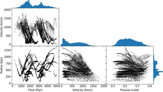
The dynamic evolution of the clumps of cold gas present in our idealized simulation. Passive scalar refers to the mass-weighted average of the passive scalar in the cells of a clump.
We define the size of a clump as the largest distance between its centre and the self-shielded cells in its bounding sphere. In the same manner, we also compute the size of its stellar content, defined as the largest such distance considering the positions of the stars within the sphere instead. The results are in Fig. 2, along with the masses of the clumps. Only a tiny minority of the clumps in the simulation contain star particles (3 per cent), and they are at the high end of the mass distribution. The extent of the stars in such clumps is smaller than that of the gas, indicating that the stars are formed at the centre of each clump and remain dynamically cold. Considering the histograms in this figure, we find that the typical gas mass of a clump is 1.6 × 10⁵ M⊙, with most clumps ranging from 2.7 × 10³ M⊙ to 4.6 × 10⁶ M⊙. The typical size of a clump is 2.2 kpc, and most clumps range from 0.3 kpc to 4.1 kpc. The latter value seems high, but we note that the largest clumps tend to simply be irregular and elongated. Among the clumps that have stars, the typical stellar mass is 107 M⊙, and the typical gas mass is 7 × 10⁶ M⊙. A second, isolated peak can be seen in the stellar mass distribution; it is associated with a single relatively large mass of gas that was ejected from one of the galaxies after it entered the cluster in an almost radial orbit and crossed its central region at high speed.
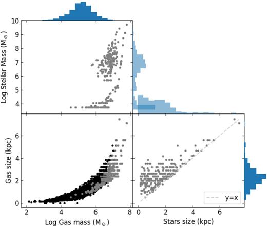
The masses and sizes of the clumps. The grey points represent clumps containing star particles, while the black ones those that do not.
3.2 Galaxies
3.2.1 Gas contamination
Using the gas cells remaining after this procedure, we extract the contamination of the ICM gas within the disc of the galaxies as they cross the cluster, as shown in Fig. 3. Some of the curves in this plot end before a complete crossing because the smallest galaxies are completely stripped. It can be seen that, after a crossing of the cluster, typically around 20 per cent of the neutral gas still in any given galaxy is actually the ICM gas that advected there – for reference, the median gas mass in the galaxies that have not been completely stripped is 39 per cent of the original gas mass. In the most extreme case, the contamination reaches more than 40 per cent, but as we will discuss in Section 3.4 using a convergence test, we cannot rule out that this particular case is spurious. Ignoring any metal deposit from stars overtime, we can extract from these values an upper bound for the predicted decrease in metallicity of the gaseous discs after one crossing of the cluster. We start by assuming the following typical metallicities: ZICM = 0.3Z⊙ (which is consistent with observational data, e.g. De Grandi & Molendi 2001) and ZISM = Z⊙ ≈ 0.02. From that we obtain a typical decrease of 14 per cent in ZISM, from 0.02 to ∼0.017.

Change in gas composition in the discs of the galaxies as they cross the cluster. Similar to Fig.1, the passive scalar value shown is a mass-weighted average. A value of 1 means that there is no contamination, and lower values represent mixing with the ICM.
3.3 Diffuse light
We compute the luminosities of the star particles formed into the clumps using the magnitude tables generated with colour–magnitude diagram (cmd, a web interface for the stellar evolution model described in Marigo et al. 2017) that are currently included in the pynbody package.4 These tables contain absolute magnitudes per solar mass in the UBVRIJHK system as a function of stellar age (assuming instantaneous star formation) and metallicity. We assume for simplicity a constant metallicity of 1 Z⊙ in our luminosity calculation, which is reasonable because the scatter in the stellar mass-metallicity relation is large (Tremonti et al. 2004), while 1 Z⊙ is a common value. The magnitudes are then interpolated from the magnitudes in the tables using the ages of the star particles.
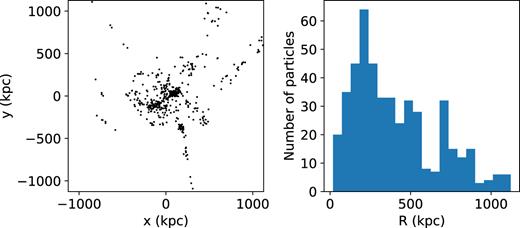
The stars formed in those most massive clumps in Fig. 2 continue to exist even after the clumps mix with the ICM. In Fig. 4, we show the spatial distribution of all such stars at the end of the simulation (z = 0). It can be noted that there is a central concentration of these stars in the cluster, for r < 500 kpc. This happens because many of the stars have had time at this point to decelerate and fall back to the centre, where they interact with each other and form a cloud. The combined MV of all the free particles is −10.8, while that of the particles within the inner 500 kpc of the cluster is −10.12. For comparison, our smallest galaxy (M200c = 1.1 × 10¹¹ M⊙) has, before entering the cluster, MV = −17.7. Clearly the luminosity of those free stars is very low, leading us to conclude that the stars associated with the clumps are an insignificant component of the diffuse light of a galaxy cluster.

All the stars formed in the clumps, which live in the ICM unattached to any galaxy, as seen at the end of the simulation. They form a cloud with radius equal to ∼500 kpc at the centre of the cluster.
3.4 Numerical convergence
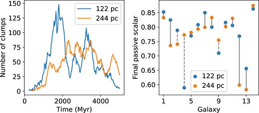
In order to assert the numerical robustness of our results, we ran our idealized simulation again with everything unchanged except for the maximum level of refinement, which was reduced by one, resulting in a maximum resolution of 244 pc (compared to the 122 pc in the main run). In principle, a higher resolution implies in less numerical diffusion, better capturing of mixing and in the possibility of resolving smaller structures. In Fig. 5, we compare the number of clumps in the cluster as a function of time for the two runs. What we observe is that in the high-resolution run, the condensation of clumps in the tails of the galaxies is visibly more intense, with more small clumps being generated. But at the same time, the mixing suppression dominates over numerical diffusion in the low-resolution run, which gives rise to the intervals in Fig.5 where there are more clumps in it. Despite of these differences, throughout most of the simulation time the number of clumps is not too different between the two runs.
Convergence test. Left: number of clumps as a function of time for the two different resolutions. Right: comparison of the mass-weighted average passive scalar in each galaxy for the two cases after one crossing of the cluster. The dashed lines indicate that in at least one of the simulations the galaxy was completely stripped before crossing.
Top of the image: a time series showing the ejection of clumps by one of our galaxies after its central passage. The time difference between each frame and the next is 100 Myr. Bottom image: a zoomed-out version of the last frame showing the galaxy and the cluster as a whole. The clumps further to the left of the image come from other galaxies. A video showing the clumps moving within the cluster overtime can be watched at http://www.astro.iag.usp.br/∼ruggiero/paperdata/2/.
Due to the high speed of our galaxies, ( >1000 km s−1), it could also be that the contamination of the ICM gas within their gaseous discs we report is partly due to numerical diffusion. So, we also compare the main simulation with the one at lower resolution to quantify this, as also shown in Fig. 5. It can be noted that our finding that a 20 per cent contamination happens after one crossing of the cluster is not resolution dependent, which implies that the accretion of the ICM gas within the gaseous discs of the galaxies must be due to the cooling of the ICM gas at the ISM/ICM interface. It should also be pointed that the most extreme case of contamination in the high-resolution run, where 40 per cent of the gas in the disc comes from the ICM, is much less pronounced in the lower resolution run, making this particular data point inconclusive.
4 DISCUSSION AND SUMMARY
We should point out that all the clump properties we obtain may have some uncertainty, given that at the clump scale processes beyond the scope of our simulations may play a crucial role in real galaxy clusters. For instance, previous simulations of cloud–shock interactions have demonstrated that the presence of magnetic fields (McCourt et al. 2015) or heat conduction (Vieser & Hensler 2007; Armillotta et al. 2017) both significantly stabilize the cloud against disruption, while both effects are absent in our simulations. Moreover, it’s possible that higher spatial resolutions would significantly change both the dynamics and the internal structure of the clumps. According to Klein et al. (1994), a resolution of ∼100 cells per cloud radius is necessary for a fully converged solution in a cloud–shock simulation; for a typical clump with radius ∼1 kpc, this would imply in a 10 pc resolution, an order of magnitude smaller than the one we have managed to reach (122 pc), despite our resolution being, for current standards, outstanding for a simulation including an entire galaxy cluster. On the other hand, recent results by Taylor et al. (2018) show that, for a cloud–shock scenario modelled after the cold clouds present in the Virgo cluster, no significant difference is found in the cloud dynamics for simulations with resolutions of 62.5 pc and 31.25 pc, which suggests that our simulation should not be too far from a converged solution. With those caveats pointed out, we believe our simulation set-up at least demonstrates that ram pressure stripping is a viable mechanism for generating lone clumps of cold gas in the ICM of galaxy clusters, although additional numerical work is needed to better constrain the internal structure and dynamics of clumps formed in this scenario.
By construction, the clumps we identify in our simulation are all self-shielded and hence composed primarily of molecular Hydrogen. The amount of neutral Hydrogen in such clumps is expected to be non-negligible (see e.g. Morris & Jura 1983), making them presumably observable using radio observations of the 21 cm line. But finding a significant number of those clumps in a cluster is not guaranteed. Their number count fluctuates overtime since their lifetime is small compared to the age of the cluster, and since most of them are generated by large structures falling into it (M200c > 1012 M⊙). In our model, that happened twice in a time span of 5 Gyr. The peak number count of clumps in the whole volume of the cluster was 148, but there were also times late in the simulation when only five clumps were present. The overall average was of 47 clumps. We have made some videos available to illustrate the process of clump generation.5
Our clumps can be associated with objects already reported in the literature. The two clouds reported in the Virgo cluster in Kent (2010) have an H i mass between 107.28 and 107.85 M⊙, at the upper end of our mass distribution, which could be either random (given the small sample size) or an observational bias towards more massive objects. Another cloud reported in the Virgo cluster in Sand et al. (2017) has a stellar mass of 5.4 ± 1.3 × 10⁴ M⊙, which is within our range of stellar masses. Its stellar age of ∼7−50Myr is relatively small compared to our clump lifetime. The clumps of molecular gas in the tail of NGC 4388 in Virgo reported in Verdugo et al. (2015) have mass between 7 × 10⁵ and 2 × 10⁶ M⊙, also within our distribution of gas masses. Similar objects found in groups of galaxies also agree with our results. In particular, Torres-Flores et al. (2009) report compact, star-forming objects with an age <100Myr in three groups, and de Mello et al. (2008) report similar objects in the Hickson Compact Group 100 with an age <200Myr. Both of these are consistent with the clump lifetime we report. The stellar mass within such objects reported by de Mello et al. (2008) is 104.3−6.5 M⊙, which is within the distribution of stellar masses that we obtain; on the other hand, their H i mass range, 109.2−10.4 M⊙, is above all of our clump masses. An important difference that should be noted between our clumps and those found in observed galaxy clusters is that the latter tend to be found preferentially at the periphery of their host clusters, while our clumps tend to be formed preferentially near the centre of the cluster (r < R200c/2); this may mean that we are underestimating the ram pressure intensity at the cluster outskirts, possibly because of the assumption of hydrostatic equilibrium (which may lead to lower relative velocities between the galaxies and the ICM).
It should be emphasized that in this work we have considered the evolution of a relatively undisturbed cluster gradually accreting small satellites overtime. But observationally, a systematic computer vision search for jellyfish morphologies (McPartland et al. 2016) has found that such systems seem to be preferably found in disturbed environments, such as cluster mergers. In such scenarios, the relative velocities between the galaxies and the surrounding medium is higher, possibly leading to higher ram pressure intensities and hence possibly different results from what we find here – for instance, the clump generation could be triggered much earlier, already at the periphery of the clusters involved, reducing the preference we find for the inner part of the cluster.
The lifetime of the clumps we find in our simulation, coupled with their fast deceleration after ejection from the galaxy, is consistent with the finding from Roediger & Brüggen (2008) that the gas lost by the galaxies tends to be deposited not far from where it was lost. One interesting inference we can make from this and from the clump dynamics we show in Fig. 1 is that the molecular gas resulting from a ram pressure stripping event is not expected to be able to feed a galaxy cluster’s central AGN since not a single clump manages to reach r = 0. The only way we can picture the infalling galaxies influencing the cluster’s AGN is if one of them fell radially and hit the black hole directly, something that to our knowledge has never been reported.
Our result that few of our clumps (3 per cent) have stars is biased since our smallest particle mass is 5.6 × 10³ M⊙. It’s possible that smaller clumps do have stars but in minute amounts not resolved by our resolution. In fact, Ohyama & Hota (2013) has managed to observe a single star in Virgo that belongs to a system analogous to the ones we describe here, a case that could not be covered by our numerical methodology. With that pointed out, the star formation inefficiency we obtain is consistent with both observations of ram pressure wakes (Verdugo et al. 2015; Jáchym et al. 2017) and with previous simulations of such systems (Tonnesen & Bryan 2012), and it is the reason why the star formation in the tails ends up being a negligible source of intracluster light.
Concerning the contamination of the discs of the galaxies with the ICM gas, we have reason to believe that the process should undergo similarly in galaxy clusters or groups across a range of masses. This is because the final contamination is roughly same for galaxies that enter our cluster with a range of different impact parameters (as robustly evidenced by our convergence test, Fig.5), and thus encounter a range of different surrounding densities, temperatures, and relative velocities. Despite those differences, the galaxies are contaminated overtime at a rather similar rate (as seen in Fig.3). This suggests that what primarily governs the contamination are not the particularities of the surrounding gas but the time since the infall of the galaxy instead.
The summary of this paper is as follows. Using a high-resolution hydrodynamic simulation of a galaxy cluster, we found that the gas stripped from infalling gas-rich galaxies gives rise to a population of clumps of molecular gas in the ICM, which live long enough to not seem obviously associated with any galaxy in the cluster. The exchange of gas also goes the other way around: an infalling galaxy advects gas from the ICM as it moves, and after one crossing of the cluster typically around 20 per cent of the gas in its disc is actually the ICM gas that ended there. We also find that the stars that form in the ram pressure tails of the galaxies are a completely negligible source of intracluster light.
Footnotes
ACKNOWLEDGEMENTS
This work is a part of the research project funded by the São Paulo Research Foundation, FAPESP (grants 15/13141-7 and 16/19586-3). GBLN thanks Conselho Nacional de Desenvolvimento Científico e Tecnológico (CNPq) for partial financial support. The simulations presented here were run at the Swiss National Supercomputing Center (CSCS), specifically using the Piz Daint supercomputer. Our data analysis has been largely done using the Hydra cluster at the University of Zurich, and it has extensively used yt (Turk et al. 2011). We thank Daisuke Nagai and Tom Abel for the suggestions that helped shape this paper.
