


ABSTRACT
We present the results of a detailed X-ray timing and spectral analysis of the BL Lacertae source OJ 287 with X-ray telescope (XRT) onboard Neil Gehrels Swift Observatory, focused on the period of its significantly enhanced X-ray flaring activity during 2016 October–2017 April. In this epoch, the 0.3–10 keV count rate from the XRT observations showed an increase by a factor of ∼10 compared to the quiescent level observed in 2016 April–May, and the mean X-ray flux was a factor of 4.5 higher than in previous years. The source underwent high X-ray flaring activity on weekly time-scales and showed 32 instances of 0.3–10 keV intraday variability (detected within the exposures shorter than 1 ks in the majority of cases) with fractional variability amplitudes of 7–60 per cent. Most of the 0.3–10 keV spectra spectra fitted well with a simple power law, yielding a wide range of the 0.3–10 keV photon index Γ = 1.90–2.90. We found 29 spectra showing an upward curvature due to the significant contribution made by the X-ray photons of inverse Compton origin. The spectral variability of OJ 287 was characterized by the dominance of a ‘softer-when-brighter’ spectral trend, explained by the emergence of a new soft component during X-ray flares. Similar to X-rays, the source underwent a strong outburst by factors of 4.6–6.5 in the optical–ultraviolet energy range which showed a positive correlation with the X-ray emission, indicating its origin to be related to the same electron population, predominantly via the synchrotron mechanism.
1 INTRODUCTION
BL Lacertae objects (BL Lacs) form an extreme subclass of blazars which are remarkable for the absence of emission lines, compact radio structure, high, and variable radio-optical polarization, apparent superluminal motion of some components, very broad continuum extending from the radio to the very high-energy (VHE) γ-rays (E > 100 GeV) and strong flux variability in all spectral bands (see Massaro, Paggi & Cavaliere 2011). According to the widely accepted scenario, a jet of magnetized plasma is launched with relativistic bulk velocity from the vicinity of a central supermassive black hole (SMBH), aligned almost along our line of sight, yielding a Doppler boosting of the observed multiwavelength (MWL) flux and decreasing the variability time-scale (Falomo, Pian & Treves 2014).
A broad-band spectral energy distribution (SED) of BL Lacs presents two different components in the log ν–log νFν plane. The lower energy ‘hump’ extends from the radio to the X-ray energy range, and its origin is widely accepted as synchrotron emission of a relativistic, magnetized plasma (Falomo et al. 2014). Based on the position of the synchrotron SED peak Ep, BL Lacs are divided into two subclasses (Padovani & Giommi 1995 and references therein): HE-peaked objects [HBLs, peaking at ultraviolet (UV)–X-ray frequencies], and low-peaked objects [LBLs, with Ep situated in the infrared (IR)–optical part of the spectrum]. Moreover, a third subclass of intermediate-energy-peaked BLLs with synchrotron peaks at optical–UV frequencies (IBLs) is also considered (Falomo et al. 2014).
However, there are various models for the origin of the SED higher energy component (extending from the X-ray to the VHE frequencies in LBLs and IBLs): (1) an inverse Compton (IC) scattering of synchrotron photons by their ‘parent’ electron–positron population (so-called synchrotron self-Compton model, SSC; Marscher & Gear 1985); (2) external Compton model (EC, Dermer,Schlickeiser & Mastichiadis 1992); and (3) hadronic models incorporating a production of γ-rays by relativistic protons, either directly (the proton synchrotron model; Mücke et al. 2003) or indirectly (e.g. synchrotron emission from a secondary electron population, produced by the interaction of HE protons with ambient photons; Mannheim 1993). A valid model can be selected through an intense MWL flux variability and interband cross-correlation study: the one-zone SSC model predicts nearly simultaneous variations in both the synchrotron and Compton components, while multizone SSC and hadronic models can explain more complicated MWL behaviour (Fossati et al. 2008).
The internal structure of BL Lacs is mostly unresolved via direct astronomical observations, and only the outer parts of relatively extended, misaligned jets are studied by the Very Long Baseline Array (VLBA; see, e.g. Rector, Gabuzda & Stocke 2003; Piner, Pant & Edwards 2010). An intensive study of MWL flux variability also is an efficient tool for evaluating the sizes of emission zones (based on the light-travel argument). A check of the MWL variability properties and interband cross-correlation aids in solving other fundamental problems, like jet launching and particle acceleration, the separation of the emission zone from the SMBH, jet matter composition, etc. Therefore, BL Lacs represent one of the favoured targets of MWL campaigns performed with different ground-based telescopes and space missions.
OJ 287 (|$z$| = 0.306, Miller, French & Hawley 1978) is one of the best studied and extensively observed in the optical range, showing regular outbursts with a period of ∼12 yr (Silampää et al. 1988; Lehto & Valtonen 1996; Valtonen et al. 2006, 2016), attributed to the central binary SMBH system in which the orbit of the secondary BH is extremely eccentric, crossing the accretion disc of the primary one twice per each encounter in every 12 yr and triggering an enhanced accretion to the primary BH which can yield the propagation of relativistic shocks though the jet. As a result, the source shows a two-peak optical outburst during each impact (Valtonen et al. 2016). This model was corroborated by radio monitoring data (Valtaoya et al. 2000) which revealed differences between the first and second bursts, hinting at the possibility that the first burst is caused by a disc-crossing while the second burst is related to enhanced accretion causing a shock front in the jet. Recently, the predicted first peak of the outburst was observed in 2015 December (which was the brightest optical level in 30 yr), followed by the comparable second peak ∼3 months later (Gupta et al. 2017). The source showed another optical outburst (expected in the case of the repeated passage of the secondary BH through the accretion disc of the primary BH) during 2017 September–December (Kushwaha et al. 2018a). Additionally, a 60-yr variability was claimed by Valtonen et al. (2006), and possible shorter term periodic behaviour in the radio–optical range was suggested by Gupta et al. (2012) and Hughes et al. (1998). Based on 120 VLBA observations during 1995 April–2017 April, Britzen et al. (2018) found that the parsec-scale radio jet of OJ287 is possibly precessing on a time-scale of ∼22 yr. Half of the jet-precession time is of order the dominant optical periodicity time-scale. In addition, the 14.5 GHz single-dish data are consistent with a jet-axis rotation on a yearly time-scale.
Recently, OJ 287 was detected at VHE γ-rays at >5 standard deviations above background during the VERITAS observations performed in 2017 February (O’Brian et al. 2017).
In this paper, we present the results of a detailed X-ray timing and spectral analysis of OJ 287 focused on the epoch of its significantly enhanced X-ray flaring activity during 2016 October–2017 April. During this period, the source was monitored extensively with X-ray telescope (XRT, Burrows et al. 2005) onboard Neil Gehrels Swift Observatory (Gehrels et al. 2004). Although these data were included in the study of Kushwaha et al. (2018a), they were used in the search for multiband correlations, as well as for the construction and modelling of the broad-band SED. On the basis of these observations, we have studied X-ray flares on time-scales from several days to a few weeks in particular parts of the aforementioned period, and checked the contemporaneous MWL behaviour of the source using all the publicly available data obtained with (i) Ultraviolet–Optical Telescope (UVOT; Roming et al. 2005) onboard Swift; (ii) Burst Alert Telescope (BAT; Barthelmy et al. 2005) onboard Swift; (iii) Monitor of All Sky X-ray Image (MAXI; Matsuoka et al. 2009); (iv) Large Area Telescope (LAT) onboard Fermi (Atwood et al. 2009); (v) various ground-based optical telescopes; and (vi) the 40-m telescope of Owens Valley Radio Observatory (OVRO; Richards et al. 2011). For comparison, we also have included the XRT observations preceding (2016 April–June) and following (2017 May–June) the epoch of strong X-ray flaring activity. We have also performed an extensive study of the X-ray variability on intraday time-scales and present the 0.3–10 keV spectra which show an upward curvature.
The paper is organized as follows. Section 2 describes the data processing and analysing procedures. In Section 3, we provide the results of a timing analysis and those from the X-ray spectroscopy in Section 4. We discuss our results in Section 5, and provide our conclusions in Section 6.
2 OBSERVATIONS AND DATA REDUCTION
2.1 X-ray data
We retrieved the raw data obtained with the grazing incidence Wolter I telescope Swift-XRT (Burrows et al. 2005) from the publicly available archive, maintained by HEASARC.1 The Level 1 unscreened XRT event files were processed with the xrtdas package developed at the ASI Science Data Center (ASDC) and distributed by HEASARC within the heasoft package (version 6.22.1). The information about each pointing and the measurement results are presented in Table 1.2 The task XRTPIPELINE was launched with standard screening criteria using the XRT CALDB calibration files version 20171113.
The XRT observations of OJ 287 in 2016 April–2017 June (extract). The columns are as follows: (1) observation ID; (2) observation beginning–end (in UTC); (3) exposure (in seconds); (4) observation mode (PC – photon counting; WT – windowed timing; (5) Modified Julian Date corresponding to the observation start; (6)–(9) mean value of the 0.3–10 keV count rate with its error (in counts s−1), reduced χ2 with the corresponding degrees of freedom, time bin used for a light-curve construction, respectively; (9) existence of a brightness variability during the observation (V stands for a variability detection; PV – possibly variable; and NV – non-variable).
| ObsID | Obs. Start–End (UTC) | Exposure (s) | Mode | MJD | CR(counts s−1) | |$\chi ^2_{\rm r}$|/d.o.f. | Bin (s) | Variability |
|---|---|---|---|---|---|---|---|---|
| (1) | (2) | (3) | (4) | (5) | (6) | (7) | (8) | (9) |
| 30901209 | 2016-04-23 02:13:58 04-23 03:17:54 | 747 | PC | 57501.10 | 0.14(0.02) | 1.13/2 | 240 s | NV |
| 30901210 | 2016-04-29 22:26:58 04-30 00:13:01 | 873 | PC | 57507.94 | 0.16(0.02) | 1.66/4 | 180 s | NV |
| 30901211 | 2016-05-06 12:22:57 05-06 13:27:45 | 770 | PC | 57514.52 | 0.11(0.02) | 2.46/3 | 180 s | NV |
| 30901212 | 2016-05-14 22:58:57 05-15 00:07:06 | 998 | PC | 57522.97 | 0.16(0.02) | 0.21/4 | 180 s | NV |
During 2016 April 23–2017 June 13, the source was targeted 143 times with XRT, yielding a total good time interval of 137 ks after the standard screening. The majority of these pointings (78 per cent) were performed in the windowed timing (WT) mode characterized by compressing 10 rows of the X-ray CCD into a single one in the serial register and then reading out only the central 200 columns of the CCD.3 We selected the events with 0–2 grades. The source and background light curves and spectra were extracted with xselect using circular areas with radii of 12–25 pixels depending on the source brightness and exposure. In the case of several observations (e. g. ObsID 30901034, 2016 November 1), the image centre of OJ 287 was just at the edge the observational area and we excluded them from our study to avoid an incorrect reconstruction of the point spread function (PSF). The light curves were then corrected using XRTLCCORR for the resultant loss of effective area, bad/hot pixels, pile-up, and vignetting. The ancillary response files (ARFs) were generated using the XRTMKARF task, with corrections for PSF losses, different extraction regions, vignetting, and CCD defects.
The large field-of-view (FOV, 1.4 sr; Barthelmy et al. 2005) instrument Swift-BAT observed OJ 287 in the 15–150 keV energy range during our period of study in the framework of the Hard X-ray Transient Monitor program5 (Krimm et al. 2013). However, the source generally is very faint in this energy range and the daily-binned data do not yield detections with 5σ significance (the threshold generally applied to coded-mask devices). Using the tool REBINGAUSSLC from heasoft, we rebinned these data within the time intervals 1–4 weeks. However, OJ 287 was detected only few times with 5σ significance in those cases and, therefore, we have not included the BAT data in our study. A similar situation occurred with the 2–20 keV observations performed with X-ray slit cameras of the MAXI mission: the publically available, weekly binned data6 do not show a detection of OJ 287 with 5σ significance.7 Using the online tool MAXI ON-DEMAND PROCESS,8 we extracted the weekly binned light curve of OJ 287 in the 2–6 keV band which generally yields the highest signal-to-noise ratios from the MAXI data, although the source was not detectable with the aforementioned significance during 2016 October–2017 June also in that case.
2.2 UV, optical, and radio observations
The results of the UVOT observations (extract). The flux values in each band are given in units of mJy.
| V | B | U | UVW1 | UVM2 | UVW2 | |||||||
|---|---|---|---|---|---|---|---|---|---|---|---|---|
| ObsId | Mag. | Flux | Mag. | Flux | Mag. | Flux | Mag. | Flux | Mag. | Flux | Mag. | Flux |
| 30901209 | 15.07(0.06) | 3.44(0.19) | 15.32(0.04) | 3.02(0.10) | 14.5(0.04) | 2.29(0.08) | 14.43(0.05) | 1.51(0.06) | 14.33(0.05) | 1.42(0.05) | 14.41(0.04) | 0.95(0.04) |
| 30901210 | 14.64(0.05) | 5.11(0.21) | 14.98(0.04) | 4.13(0.13) | 14.21(0.04) | 2.99(0.11) | 14.08(0.04) | 2.09(0.09) | 14.04(0.04) | 1.85(0.05) | 4.22(0.04) | 1.13(0.05) |
| 30901211 | 14.94(0.06) | 3.87(0.20) | 15.23(0.04) | 3.28(0.12) | 14.44(0.04) | 2.42(0.08) | 14.31(0.05) | 1.69(0.08) | 14.24(0.05) | 1.54(0.05) | 14.44(0.04) | 0.92(0.04) |
| 30901212 | 14.87(0.05) | 4.13(0.18) | 15.32(0.04) | 3.02(0.09) | 14.51(0.04) | 2.27(0.08) | 14.42(0.04) | 1.53(0.06) | 14.37(0.05) | 1.37(0.04) | 14.55(0.04) | 0.83(0.04) |
The ranges of the 0.3–10 keV count rates of the most frequently observed LBLs/IBLs. In the last column, the reference S13 stands for Stroh & Falcone (2013), and TW: this work.
| Source | |$z$| | CRmin | CRmax | Reference |
|---|---|---|---|---|
| (1) | (2) | (3) | (4) | (5) |
| S5 0716 + 714 | 0.300 | 0.11(0.01) | 2.05(0.05) | S13 |
| BL Lacs | 0.069 | 0.11(0.01) | 1.92(0.05) | S13 |
| OJ 287 | 0.306 | 0.05(0.01) | 1.89(0.03) | S13, TW |
| VER J0521 + 212 | – | 0.026(0.006) | 1.69(0.27) | S13 |
| 3C 66A | 0.340 | 0.06(0.01) | 1.59(0.41) | S13 |
| AO 0235 + 16 | 0.940 | 0.012(0.004) | 1.23(0.05) | S13 |
| W Comae | 0.103 | 0.022(0.007) | 0.91(0.21) | S13 |
| S4 0954 + 65 | 0.367 | 0.05(0.01) | 0.87(0.03) | S13 |
| OT 81 | 0.322 | 0.07(0.01) | 0.78(0.03) | S13 |
| S3 1227 + 25 | 0.135 | 0.27(0.01) | 0.67(0.03) | S13 |
| S2 0109 + 22 | 0.265 | 0.06(0.01) | 0.65(0.02) | S13 |
| QSO B1514 − 24 | 0.049 | 0.11(0.01) | 0.54(0.04) | S13 |
| PKS 0537 − 441 | 0.892 | 0.06(0.01) | 0.51(0.05) | S13 |
The OVRO 40-m telescope uses off-axis dual-beam optics and a cryogenic high electron mobility transistor (Richards et al. 2011). The regular OVRO observations of OJ 287 at the frequency 15.0 GHz have been carried out since 2008 January 9. We retrieved the publicly available OVRO data of our target from the corresponding website.11 The details of the data reduction and calibration procedure can be found in Richards et al. (2011).
We also have used the archival 15 GHz data obtained in the framework of Monitoring Of Jets in Active galactic nuclei with VLBA Experiments12 (MOJAVE). The details of the data reduction and calibration procedure are provided in Lister et al. (2009). For the construction of long-term radio light curve, we also used the 14.5 GHz observations performed with the the 26-m telescope of University of Michigan Radio Astronomy Observatory13 (UMRAO; see Aller et al. 1985 for details).
2.3 γ-ray observations
Fermi-LAT generally monitors the entire sky in the energy range of 20 MeV–300 GeV every 3 h, and this instrument is characterized by the energy resolution better than 10 per cent and an FOV of ∼2.4 sr, with an angular resolution (68 per cent containment angle) better than 1 deg at the energies higher than 1 GeV (Atwood et al. 2009). We extracted the 0.1–300 GeV fluxes from the LAT observations selecting the events of the diffuse class from a region of interest (ROI) of radius 10 deg, centred on OJ 287, and processed with the Fermisciencetools package version v11r5p3. For this purpose, we used the instrument response function and P8R2_V6 and the unbinned maximum likelihood method GTLIKE.14 A cut on the zenith angle (>100 deg) was done to reduce contamination from the Earth-albedo γ-rays. The data taken when the rocking angle of the spacecraft is larger than 52 deg are discarded to avoid a contamination from the Earth’s limb photons.
A background model including all γ-ray sources from the Fermi-LAT 4-yr point source catalogue (3FGL, Acero et al. 2015) within 20 deg of OJ 287 was created. The spectral parameters of sources within the ROI were left free during the minimization process, while those outside of this range were fixed to the 3FGL catalogue values. The Galactic and extragalactic diffuse γ-ray emission as well as the residual instrumental background were included using the recommended model files gll_iem_v06.fits and iso_P8R2_SOURCE_V6_v06.txt. The normalizations of both components in the background model were allowed to vary freely during the spectral fitting. For the spectral modelling of our target, we adopted a log-parabola model, as done in the 3FGL catalogue. Its detection significance σ was then calculated as σ ≈ (TS)1/2 (Abdo et al. 2009). When the source was not detectable at the 3σ significance, we calculated the upper limit to the photon flux using the CALCUPPER tool included in the user-contributed package latanalysisscripts (version 0.2.1).15
3 FLUX VARIABILITY
3.1 Long-term X-ray and MWL flux variability 2016 April–2017 June
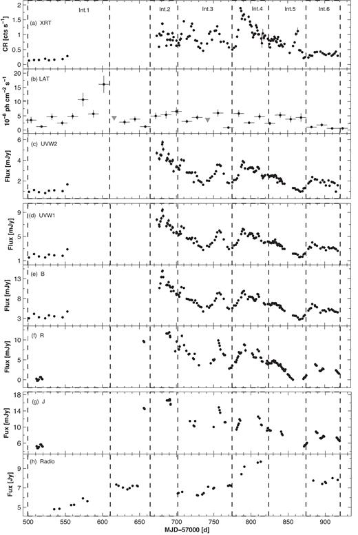
OJ 287 showed a strong X-ray outburst during 2016 October–2017 April: the 0.3–10 keV count rate from the XRT observations showed an increase by a factor of ∼10 on 2016 October 19 (MJD 57681) compared to the quiescent level in the 2016 April–May period (Fig. 1a). Consequently, it became the sixth LBL/IBL source with the rate higher than 1 counts s−1 (after S5 0716 + 714, BL Lacs, 3C 66A, VER J0521 + 212, and AO 0235 + 16; see Table 3).Afterwards, the source continued a strong X-ray flaring activity on weekly time-scales and attained its highest historical 0.3–10 keV brightness corresponding to 1.89 ± 0.03 counts s−1 on 2017 February 2 (MJD 57786; see Fig. 2a). The mean count rate during 2016 October–2017 April |$\overline{\text{CR}}$| = 0.932 ± 0.002 counts s−1, while this quantity was 4.5 times smaller during the previous 300 XRT observations of OJ 287 and the highest 0.3–10 keV rate was 0.38 ± 0.10 counts s−1 in that period (recorded on 2009 March 5; MJD 54896). Along with the strong optical outbursts in 2005–2006 and 2015 December–May (attributed to the impact of the secondary BH to the accretion disc of the primary one; see Figs 1e–f), the source showed low X-ray activity.16 Unfortunately, the source was not observed with Swift for almost 4 months due to the Sun constraint during 2016 June14–October 11 when it showed high states in the optical R band, IRJ band, and at 15 GHz (see Figs 2f–h, as well as Kushwaha et al. 2018a, Valtonen et al. 2017 and the R-band light curve provided on the website of Tuorla Observatory17).

Historical light curves of OJ 287 from the MWL observations in 2005–2017 with XRT (top panel), Fermi-LAT (panel b), UVOT bands UVW2, UVW1, and B (panels c–e), R band of the Johnson–Cousins system (various ground-based telescopes; panel f), IR J band with the SMARTS 1.3-m telescope (panel g), and radio observations with the UMRAO and OVRO telescopes (panel h). In the latter case, grey and black points are used for the UMRAO and OVRO data, respectively. For the LAT observations, we used two-weekly bins, while daily bins are adopted for those performed with other facilities. Grey triangles in panel (b) represent 2σ upper limits to the LAT flux when the source was detected below the 3σ significance. The 2016 April–2017 June period is indicated by vertical dashed lines.
The same as Fig. 1 for the period 2016 April–2017 June. The triangles in panel (b) stand for 2σ upper limits to the LAT flux when the source was detected below the 3σ significance. The vertical dashed lines indicate the periods discussed in Section 3.2.
Similar to X-rays, the source showed a strong outburst by factors of 4.6–6.5 in the UVOT bands V–UVW2 (Figs 1c–e) in 2016 October and kept its high optical–UV states during the next months, although its flaring activity was not as strong as in the 0.3–10 keV energy range in this period (see Figs 2c–e). A similar behaviour was observed also in the optical R and IR J bands, although the flare in 2016 October was characterized by lower amplitudes (by factors of 2.7–3.5) compared to those at the higher frequencies (Figs 2f–g). Finally, a radio-band flare by a factor of 2.9 was observed along with the X-ray one and the source showed its 15 GHz peak on MJD 57813, delayed by 27 d from the highest historical 0.3–10 keV state (see Figs 1h and 2h). Moreover, OJ 287 exhibited its lower radio states during the UV–IR outburst in 2015 December–2016 May.
Since the start of Fermi operations (2008 August), OJ 287 mostly was a faint γ-ray source at HE γ-rays (E >1 MeV) and, therefore, we had to use two-weekly LAT binned data to construct the historical 0.1–300 GeV light curve (Fig. 1b). However, the source was not detectable with 3σ significance or the parameter Nped (the predicted number of the photons) showed values less than 10 (yielding less credible values of the derived photon flux; see, e.g. Raiteri et al. 2013) on 22 occasions, and we plotted a 2σ upper limit in Figs 1(b) and 2(b). In the case of one-weekly binned LAT data, we applied 2σ upper limits to the 0.1–300 GeV flux in 43 per cent of the cases during 2016 April–2017 June (see Table 4). In contrast to other spectral bands, the source did not show an outburst in the LAT energy range during the here-presented period and underwent only a moderate 0.1–300 GeV flare in 2016 July–August when it was not observed with Swift. On average, the LAT-band flux in 2016 October–2017 April was one of the lowest during the entire 2008–2017 period, and the source showed its strongest γ-ray outburst during MJD 55800–56920 (2011 August–December): the 0.1–300 GeV flux exceeded a level of 5 × 10⁻⁷photons cm−2 s−1 (see Fig. 1b) and was brighter than 10−6photons cm−2 s−1 when using shorter time bins (Hodgson et al. 2017).
The results from the one-weekly binned LAT observations of OJ 287 in 2016 April–2017 June. In column (3), the 0.1–300 GeV flux is given in units of 10−8photons cm−2 s−1, and the upper limits to the flux are shown along with an asterisk; column (4), the photon index at the reference energy E0 fixed to the 3FGL catalogue value; column (5), the curvature parameter; column (6), the number of the photon predicted by the model; and column (7), the test statistics corresponding to OJ 287.
| Dates | MJD-57000 | F0.1-300GeV | α | β | Npred | TS |
|---|---|---|---|---|---|---|
| (1) | (2) | (3) | (4) | (5) | (6) | (7) |
| 2016–Apr 23-30 | 501–508 | 2.84(1.04) | 2.50(0.21) | 0.47(0.23) | 12.5 | 10.1 |
| Apr 30–May 7 | 508–515 | 5.42(1.30) | 2.59(0.15) | 0.63(0.20) | 23.8 | 30.4 |
| May 7–14 | 515–522 | 6.10* | – | – | 1.0 | 3.6 |
| May 14–21 | 522–529 | 5.02* | – | – | 0.9 | 5.6 |
| May 21–28 | 529–536 | 4.57(1.27) | 1.88(0.19) | 0.28(0.14) | 16.6 | 20.9 |
| May 28–June 4 | 536–543 | 7.24(1.80) | 2.20(0.18) | 0.06(0.14) | 27.8 | 22.2 |
| June 4–11 | 543–550 | 5.11* | – | – | 8.9 | 15.1 |
| June 11–18 | 550–557 | 2.66(0.70) | 1.83(0.19) | 0.43(0.18) | 15.8 | 23.5 |
| June 18–25 | 557-564 | 4.93(1.10) | 1.92(0.18) | 0.43(0.15) | 22.2 | 32.4 |
| June 25–July 2 | 564–571 | 7.69(2.04) | 2.76(0.20) | 0.51(0.21) | 25.0 | 13.4 |
| July 2–9 | 571–578 | 4.84(1.45) | 2.20(0.21) | 0.02(0.17) | 10.1 | 15.5 |
| July 9–16 | 578–585 | 13.04(2.76) | 2.58(0.17) | 0.50(0.16) | 45.8 | 31.8 |
| July 16–23 | 585–592 | 9.57* | – | – | 9.95 | 27.2 |
| July 23–30 | 592–599 | 6.63(1.4) | 1.97(0.16) | 0.01(0.15) | 27.3 | 31.3 |
| July 30–Aug 6 | 599–606 | 14.74(2.91) | 2.03(0.13) | 0.02(0.14) | 56.9 | 43.0 |
| Aug 6–13 | 606–613 | 7.18(1.85) | 2.04(0.17) | 0.01(0.17) | 22.3 | 24.4 |
| Aug 13–20 | 613–620 | 7.05* | – | – | 12.3 | 8.9 |
| Aug 20–27 | 620–627 | 6.21* | – | – | 6.5 | 10.0 |
| Aug 27–Sept 3 | 627–634 | 5.3(1.67) | 1.84(0.20) | 0.39(0.20) | 23.3 | 12.8 |
| Sept 3–10 | 634–641 | 5.03* | – | – | 1.8 | 7.5 |
| Sept 10–17 | 641–648 | 3.88(0.83) | 1.88(0.15) | 0.45(0.15) | 23.3 | 41.4 |
| Sept 17–24 | 648–655 | 4.13* | – | – | 7.6 | 9.8 |
| Sept 24–Oct 1 | 655–662 | 3.72* | 2.10(0.21) | 0.45(0.22) | 12.2 | 10.1 |
| Oct 1–8 | 662–669 | 8.21(1.66) | 2.07(0.14) | 0.02(0.13) | 30.9 | 40.6 |
| Oct 8–15 | 669-676 | 2.17(0.48) | 2.38(0.18) | 0.40(0.18) | 12.9 | 33.3 |
| Oct 15–22 | 676–683 | 4.29* | – | – | 0.7 | 3.8 |
| Oct 22–29 | 683–690 | 8.35(2.34) | 2.46(0.19) | 0.18(0.19) | 27.3 | 15.5 |
| Oct 29–Nov 5 | 690–697 | 7.34(2.12) | 2.58(0.18) | 0.43(0.18) | 27.4 | 20.6 |
| Nov 5–12 | 697–704 | 7.94* | – | – | 20.7 | 8.85 |
| Nov 12–19 | 704–711 | 3.72(0.72) | 2.56(0.13) | 0.38(0.12) | 26.2 | 73.9 |
| Nov 19–26 | 711–718 | 3.36(1.1) | 1.94(0.21) | 0.30(0.19) | 17.6 | 14.4 |
| Nov 26–Dec 3 | 718–725 | 2.19(0.45) | 2.24(0.19) | 0.37(0.15) | 14.8 | 55.7 |
| Dec 3–10 | 725–732 | 6.47(1.33) | 1.93(0.13) | 0.39(0.13) | 32.2 | 60.8 |
| Dec 10–17 | 732–739 | 5.53* | – | – | 0.2 | 0.9 |
| Dec 17–24 | 739–746 | 4.71* | – | – | 3.6 | 29.4 |
| Dec 24–31 | 746–753 | 5.04* | – | – | 4.6 | 10.2 |
| Dec 31–2017 Jan 7 | 753–760 | 4.64(1.04) | 1.87(0.14) | 0.51(0.14) | 22.9 | 50.1 |
| Jan 7–14 | 760–767 | 10.81(2.14) | 2.67(0.16) | 0.01(0.15) | 15.3 | 34.3 |
| Jan 14–21 | 767–774 | 7.10* | – | – | 7.4 | 24.8 |
| Jan 21–28 | 774–781 | 2.87(0.61) | 1.81(0.15) | 0.24(0.14) | 15.7 | 46.2 |
| Jan 28–Feb 4 | 781–788 | 4.55(1.17) | 19.7(0.17) | 0.10(0.16) | 19.7 | 25.5 |
| Feb 4–11 | 788–795 | 7.24(1.60) | 1.95(0.14) | 0.01(0.14) | 28.6 | 45.9 |
| Feb 11–18 | 795–802 | 6.38* | – | – | 9.0 | 17.0 |
| Feb 18–25 | 802–809 | 2.63(0.75) | 1.84(0.18) | 0.08(0.17) | 13.3 | 20.9 |
| Feb 25–Mar 2 | 809–816 | 5.21(1.67) | 2.03(0.18) | 0.02(0.16) | 23.0 | 22.5 |
| Mar 4–11 | 816–823 | 2.70(0.51) | 1.83(0.12) | 0.12(0.12) | 31.4 | 79.3 |
| Mar 11–18 | 823–830 | 3.98* | – | – | 5.5 | 11.3 |
| Mar 18–25 | 830–837 | 5.15(0.95) | 1.87(011) | 0.01(0.11) | 25.3 | 88.5 |
| Mar 25–Apr 1 | 837–844 | 4.74(1.1) | 1.93(0.16) | 0.33(0.15) | 22.1 | 28.8 |
| Apr 1–8 | 844-851 | 4.48* | – | – | 4.3 | 14.0 |
| Apr 8–15 | 851–858 | 7.42(2.30) | 2.25(0.17) | 0.02(0.18) | 31.0 | 17.6 |
| Apr 15–22 | 858–865 | 8.55(2.5) | 2.38(0.17) | 0.01(0.18) | 29.5 | 14.2 |
| Apr 22–29 | 865–872 | 7.31* | – | – | 10.2 | 8.3 |
| Apr 29–May 6 | 872–879 | 4.44* | – | – | 1.8 | |
| May 6–13 | 879–886 | 3.71* | – | – | 5.7 | 17.1 |
| May 13–20 | 886–893 | 5.19* | – | – | 6.9 | 9.0 |
| May 20–27 | 893–900 | 3.39* | – | – | 1.9 | 7.5 |
| May 27–June 3 | 900–907 | 3.38* | - | – | 0.4 | 1.9 |
| June 3–10 | 907–914 | 3.02* | – | – | 8.3 | 37.5 |
| June 10–17 | 914–921 | 2.28* | – | – | 2.25 | 9.2 |
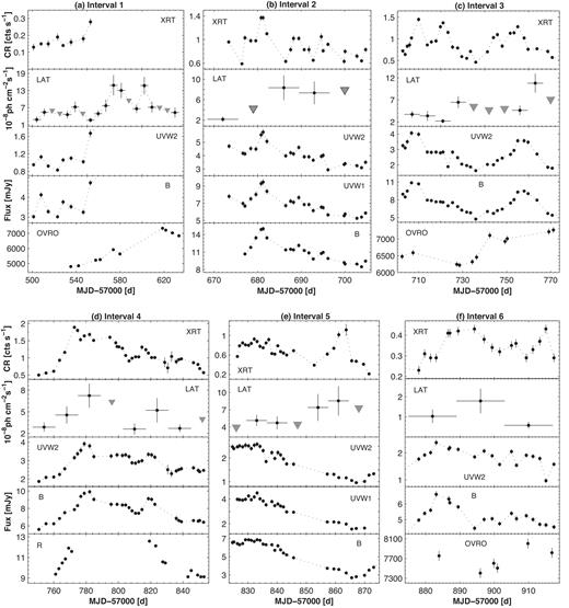
The variability of the MWL flux in different intervals. Grey triangles in LAT-band panels stand for upper limits to the LAT flux when the source was detected below 3σ significance.
Summary of the XRT and UVOT observations in different periods. Columns 3 and 4: maximum 0.3–10 keV flux (in counts s−1) and maximum-to-minimum flux ratio, respectively; maximum unabsorbed flux (in 10−11erg cm−2s−1) and fractional variability amplitude (in percent) in 2–10 keV (columns 5 and 6) and 0.3–2keV (columns 7 and 8) bands; and columns 9–20: maximum-to-minimum flux ratio and fractional amplitude in the UVOT bands.
| XRT | UVOT | ||||||||||||||||||
|---|---|---|---|---|---|---|---|---|---|---|---|---|---|---|---|---|---|---|---|
| Int. | Dates | CRmax | R | |$F^{\rm max}_{\rm 2-10}$| | Fvar | |$F^{\rm max}_{\rm 0.3-2}$| | Fvar | |$F^{\rm max}_{\rm W2}$| | Fvar | |$F^{\rm max}_{\rm M2}$| | Fvar | |$F^{\rm max}_{\rm W1}$| | Fvar | |$F^{\rm max}_{\rm U}$| | Fvar | |$F^{\rm max}_{\rm B}$| | Fvar | |$F^{\rm max}_{\rm V}$| | Fvar |
| (1) | (2) | (3) | (4) | (5) | (6) | (7) | (8) | (9) | (10) | (11) | (12) | (13) | (14) | (15) | (16) | (17) | (18) | (19) | (20) |
| 1 | 2016 Apr 23–Sept 2 | 0.23 | 2.1 | 0.28 | 24.6(13.3) | 0.54 | 21.5(5.6) | 1.67 | 23.1(1.7) | 2.63 | 22.9(1.0) | 2.88 | 22.4(1.6) | 4.02 | 19.9(1.2) | 4.74 | 16.3(1.2) | 6.31 | 18.7(1.6) |
| 2 | 2016 Oct 7–Nov 12 | 1.14 | 2.4 | 1.16 | 39.4(5.4) | 2.77 | 25.3(1.5) | 5.75 | 17.2(0.9) | 8.79 | 18.1(0.5) | 9.46 | 16.2(0.8) | 12.25 | 16.0(0.7) | 15.0 | 16.3(0.5) | 19.09 | 15.3(0.8) |
| 3 | 2016 Nov 12–2017 Jan 17 | 1.32 | 3.7 | 1.07 | 27.7(2.9) | 2.87 | 36.5(1.3) | 4.06 | 25.8(0.8) | 6.31 | 26.4(0.6) | 6.67 | 23.9(0.8) | 8.95 | 24.1(1.6) | 10.86 | 21.4(0.5) | 13.43 | 20.5(0.6) |
| 4 | 2017 Jan 20–Mar 13 | 1.67 | 4.4 | 1.30 | 33.0(2.4) | 4.05 | 42.6(1.1) | 3.91 | 17.7(0.8) | 5.86 | 17.2(0.5) | 6.25 | 16.4(0.7) | 8.02 | 15.0(0.5) | 9.91 | 14.8(0.5) | 12.13 | 15.4(0.6) |
| 5 | 2017 Mar 13–Apr 29 | 0.77 | 3.9 | 0.82 | 28.2(4.6) | 1.38 | 23.5(1.8) | 2.58 | 29.1(1.9) | 3.94 | 29.6(0.6) | 4.49 | 28.7(0.8) | 5.65 | 28.4(0.6) | 6.85 | 27.4(0.5) | 8.55 | 26.9(0.7) |
| 6 | 2017 May 1–June 13 | 0.40 | 1.9 | 5.37 | 6.7(9.5) | 0.92 | 9.3(3.2) | 2.38 | 13.2(1.0) | 3.56 | 13.6(0.6) | 4.02 | 12.2(1.0) | 5.15 | 12.2(0.8) | 6.61 | 12.9(0.7) | 7.94 | 11.4(0.9) |
3.2 Shorter term flares
During interval 1 (see Table 5 for the corresponding time range), the source was observed only eight times with Swift, showing a typical 0.3–10 keV level corresponding to CR ∼0.15 counts s−1 and a brightening by ∼50 per cent during the last two XRT pointings (Fig. 3a, top panel). A similar behaviour was observed also during the contemporaneous optical–UV observations, although a low-amplitude flare was observed in this energy range in the beginning of this period (see panels 4 and 5). Meanwhile, OJ 287 demonstrated lower LAT-band states and showed an HE peak 3 weeks after the last XRT pointing. During interval 1, the 15 GHz brightness underwent a long-term increase and exhibited its highest level with ∼1.5 months delay with respect to the LAT-band peak.
At the beginning interval 2, the source was found in a highly elevated X-ray state, superimposed by shorter term flares. Namely, it showed a flare by a factor of 2.3 in 5 d, followed by a drop to the initial level in the same time (Fig. 3b). A similar behaviour was observed also in the optical–UV energy range. Afterwards, the source underwent two subsequent lower amplitude X-ray flares along with long-term optical–UV decline. Two subsequent, double-peak flares by factors of 2.3–2.8 occurred in interval 3 (Fig. 3c). The source showed optical–UV flares along with X-ray ones, although the corresponding light curves do not show a double-peak structure. The 15 GHz flux showed an increase along with the second X-ray flare, while the LAT band did not exhibit any correlation with those in other energy ranges.
In interval 4, the 0.3–10 keV rate increased by a factor of 3.1 in 6 d to the highest historical level, and then showed a much longer decline to the initial level (lasting ∼40 d), superimposed by low-amplitude brightness fluctuations (Fig. 3d). The optical–UV light curves show a correlated behaviour, although with some time shifts. The highest LAT-band state was observed in the epoch of the highest UVOT-band states, although the brightness increase was considerably smaller (followed by uncorrelated variability). Two subsequent X-ray flares were observed in interval 5 and the second, considerably stronger one was not accompanied by enhanced activity in the optical–UV energy range: the source exhibited a long-term declining trend in that epoch (Fig. 3e).
In interval 6, the source did not show as high X-ray states as in the previous intervals, and its behaviour was characterized by brightness enhancements by only 40–80 per cent on weekly time-scales (Fig. 3f). The optical–UV fluxes showed little correlation with the 0.3–10 keV one and the source did not exhibit a significant variability (similarly to the previous time interval).
3.2.1 Intraday variability
We have also performed an intensive search for intraday X-ray variability (IDV, i.e. a flux change within a day; see Wagner & Witzel 1995) from the XRT observations performed during 2016 April–2017 June, using the χ2-statistics introduced by Kesteven, Bridle & Brandie (1976). For light-curve construction, we used time bins of 60–240 s (depending on the target’s brightness) and performed bin-per-bin subtraction of the background signal from the source one (by means of the xronos task LCURVE, included in heasoft).
The source showed 32 instances of 0.3–10 keV IDVs whose summary is provided in Table 6. The latter contains the values of reduced χ2, fractional variability amplitude, the ranges of the spectral parameters a, b, Ep, and HR (defined in Section 4) for each instance, derived from separate orbits or segments of the corresponding XRT observation.
Summary of the 0.3–10 keV IDVs in 2016 April–2017 June. The third column gives the total observation duration (including the intervals between the orbits). In column (7), the acronym ‘LP’ denotes ‘log-parabolic’ fit, and ‘PL’ – ‘power-law’ fit.
| ObsID(s) | Dates | ΔT(h) | |$\chi ^2_{\rm r}$|/d.o.f. | Bin | Fvar(percent) | a | b | HR |
|---|---|---|---|---|---|---|---|---|
| (1) | (2) | (3) | (4) | (5) | (6) | (7) | (8) | (9) |
| 99.9 per cent | ||||||||
| 30901(220-221) | 2016 Oct 15/16 | 22.90 | 54.76/1 | Orbit | 32.6(3.2) | 2.65(0.09)–2.81(0.08) PL | – | 0.20(0.03)–0.27(0.04) |
| 30901221 | 2016 Oct 16 | 0.25 | 5.09/4 | 180 s | 19.2(4.3) | 2.81(0.08) PL | – | 0.20(0.03) |
| (30901)225–226 | 2016 Oct 19/20 | 13.30 | 12.77/2 | Orbit | 13.5(2.3) | 2.78(0.06) LP, 2.82(0.08)-2.90(0.07) PL | −0.42(0.18) | 0.17(0.02)–0.28(0.04) |
| 30901226 | 2016 Oct 20 | 2.48 | 11.28/1 | Or | 13.4(3.0) | 2.82(0.08)-2.90(0.07) PL | – | 0.17(0.02)–0.20(0.03) |
| (30901)226–227 | 2016 Oct 20/21 | 22.47 | 4.13/3 | Orbit | 7.4(2.1) | 2.82(0.08)-2.90(0.07) PL | – | 0.17(0.02)–0.20(0.03) |
| 30901227 Orbit 1 | 2016 Oct 21 | 0.23 | 5.94/9 | 120 s | 23.2(4.3) | 2.85(0.08) PL | – | 0.19(0.03) |
| (30901)229–230 | 2016 Oct 26/27 | 17.08 | 21.13/1 | Orbit | 21.6(3.5) | 2.71(0.09) LP, 2.70(0.10) PL | −0.52(0.27) | 0.25(0.04)–0.34(0.07) |
| 30901232 | 2016 Oct 29 | 0.30 | 3.68/8 | 120 s | 20.2(4.5) | 2.84(0.09) PL | – | 0.25(0.04) |
| 30901237 | 2016 Nov 03 | 0.27 | 3.58/7 | 120 s | 19.2(4.8) | 2.83(0.09) LP | −0.59(0.30) | 0.29(0.06) |
| 30901250 | 2016 Nov 23 | 0.27 | 3.59/7 | 120 s | 17.9(4.5) | 2.58(0.07) PL | – | 0.30(0.04) |
| 30901253 | 2016 Nov 29 | 0.27 | 3.59/7 | 120 s | 16.3(3.8) | 2.60(0.06) LP | −0.44(0.16) | 0.39(0.05) |
| 33756090 | 2016 Dec 05 | 0.27 | 5.06/7 | 120 s | 25.7(4.7) | 2.50(0.09) PL | – | 0.35(0.06) |
| 33756093 | 2016 Dec 11 | 0.27 | 4.76/7 | 120 s | 37.2(6.7) | 2.71(0.11) LP | −0.66(0.28) | 0.40(0.08) |
| 33756107 | 2017 Jan 17 | 0.27 | 3.97/7 | 120 s | 33.0(7.2) | 2.31(0.16) PL | – | 0.49(0.12) |
| 33756113 | 2017 Jan 30 | 0.27 | 3.70/7 | 120 s | 18.3(4.2) | 2.35(0.07) PL | – | 0.46(0.05) |
| 33756114 | 2017 Jan 30 | 0.53 | 3.21/15 | 120 s | 11.5(2.3) | 2.50(0.04) PL | – | 0.35(0.02) |
| 34934002 | 2017 Feb 16 | 0.27 | 3.49/7 | 120 s | 14.7(3.9) | 2.73(0.09) PL | – | 0.22(0.03) |
| 34934003 | 2017 Feb 17 | 0.27 | 3.48/7 | 120 s | 15.6(4.1) | 2.54(0.07) PL | – | 0.31(0.04) |
| 34934004 | 2017 Feb 18 | 0.33 | 3.38/9 | 120 s | 16.7(3.9) | 2.56(0.06) PL | – | 0.30(0.03) |
| 34934005 | 2017 Feb 19 | 0.27 | 3.82/7 | 120 s | 20.9(4.7) | 2.55(0.08) PL | – | 0.22(0.03) |
| 34934006 | 2017 Feb 20 | 0.30 | 3.19/8 | 120 s | 17.7(4.4) | 2.68(0.07) LP | −0.40(0.20) | 0.31(0.04) |
| 34934007 | 2017 Feb 21 | 0.27 | 4.44/7 | 120 s | 22.0(4.7) | 2.75(0.07) LP | −0.86(0.20) | 0.41(0.05) |
| 34934008 | 2017 Feb 22 | 0.27 | 4.20/7 | 120 s | 23.9(4.8) | 2.30(0.08) PL | – | 0.47(0.06) |
| 34934021 | 2017 Mar 07 | 0.17 | 4.67/4 | 120 s | 22.6(5.7) | 2.54(0.09) PL | – | 0.31(0.05) |
| 34934022 | 2017 Mar 11 | 0.27 | 6.41/7 | 120 s | 32.4(5.2) | 2.63(0.09) LP | −0.73(0.24) | 0.48(0.08) |
| 34934023 | 2017 Mar 12/13 | 15.73 | 54.38/1 | Orbit | 59.7(5.8) | 2.72(0.09) LP, 2.33(0.13) PL | −0.86(0.23) | 0.45(0.09)–0.46(0.08) |
| 34934027 | 2017 Mar 16 | 0.27 | 5.59/7 | 120 s | 38.5(5.9) | 2.30(0.11) PL | – | 0.47(0.08) |
| 34934030 | 2017 Mar 19 | 0.27 | 3.54/7 | 120 s | 26.0(6.3) | 2.37(0.10) PL | – | 0.42(0.07) |
| 34934032 | 2017 Mar 21 | 0.27 | 3.80/7 | 120 s | 24.8(5.6) | 2.36(0.10) PL | – | 0.42(0.07) |
| 34934033 | 2017 Mar 22 | 0.27 | 4.94/7 | 120 s | 37.2(6.9) | 2.32(0.11) PL | – | 0.56(0.10) |
| 34934035 | 2017 Mar 24 | 0.27 | 4.07/7 | 120 s | 24.7(4.9) | 2.39(0.10) PL | – | 0.41(0.06) |
| 34934039 | 2017 Mar 28 | 2.99 | 16.53/1 | 120 s | 25.6(4.7) | 2.66(0.19)–2.85(0.15) PL | – | 0.18(0.05)–0.26(0.08) |
| 34934041 | 2017 Mar 30 | 0.27 | 4.26/7 | 120 s | 38.7(8.4) | 2.73(0.18) PL | – | 0.33(0.05) |
| 34934046 | 2017 Apr 18 | 0.17 | 4.82/4 | 120 s | 38.7(7.7) | 2.71(0.14) LP | −0.82(0.37) | 0.39(0.10) |
| 99.5 per cent | ||||||||
| 30901222 | 2016 Oct 17 | 0.27 | 2.94/7 | 120 s | 12.4(3.4) | 2.65(0.09)PL | – | 0.27(0.04) |
| 30901225 | 2016 Oct 19 | 0.27 | 2.1/7 | 120 s | 13.7(4.0) | 2.78(0.06) LP | −0.42(0.18) | 0.28(0.04) |
| 30901226 Orbit 2 | 2016 Oct 20 | 0.23 | 3.22/6 | 120 s | 16.6(5.1) | 2.82(0.08) PL | – | 0.20(0.03) |
| 30901245 | 2016 Nov 12 | 0.27 | 3.01/7 | 120 s | 20.1(5.9) | 2.60(0.09) PL | – | 2.29(0.04) |
| 30901(246-247) | 2016 Nov 13/14 | 21.95 | 8.48/1 | Orbit | 15.6(4.2) | 2.51(0.07)–2.73(0.18) PL | – | 0.23(0.07)–0.29(0.04) |
| 30901255 | 2016 Dec 03 | 0.20 | 3.38/5 | 120 s | 26.0(6.7) | 2.48(0.14) PL | – | 0.36(0.08) |
| (349340)25-26 | 2017 Mar 14/15 | 18.67 | 8.50/1 | Orbit | 17.8(4.7) | 2.51(0.11) LP, 2.38(0.18) PL | −0.64(0.29) | 0.41(0.12)–0.56(0.08) |
| 34934028 | 2017 Mar 17 | 0.30 | 2.82/8 | 120 s | 27.0(6.9) | 2.49(0.10) LP | −0.64(0.21) | 0.62(0.07) |
| 34934031 | 2017 Mar 20 | 0.23 | 3.42/6 | 120 s | 19.4(6.1) | 2.31(0.09) PL | – | 0.46(0.07) |
| 34934036 | 2017 Mar 25 | 0.27 | 2.98/7 | 120 s | 16.0(4.5) | 2.76(0.09) LP | −0.78(0.25) | 0.39(0.07) |
| 34934043 | 2017 Apr 02 | 0.23 | 3.26/6 | 120 s | 18.3(6.5) | 2.42(0.11) LP | −0.87(0.32) | 0.86(0.16) |
Figs 4(a)–(c) present the X-ray behaviour of the source during its most densely sampled observations performed during 2017 March 11–31, with a total exposure of 20.8 ks distributed over 22 XRT pointings. During this campaign, the source showed nine IDVs (see Table 6): a flux variability within 1 ks exposures was recorded during ObsIDs 34934022 and 34934027 (panels 1 and 6 of Fig. 4a, respectively); ObsIDs 34934030, 34934032, 34934033, and 34934035 (panels 2, 4, 5, and 7 of Fig. 4b, respectively);ObsIDs 34934039 and 34934041 (panels 4 and 6 of Fig. 4c, respectively). Moreover, two another IDVs occurred between two different orbits of ObsID 34934023 (panel 2 of Fig. 4a). These instances were characterized by Fvar = 24.7(4.9)–59.7(5.8) per cent and ranges of the spectral parameters (see Section 4.1 for their definitions): Γ = 2.30(0.11)–2.85(0.15), and HR = 0.18(0.05)–0.56(0.10).
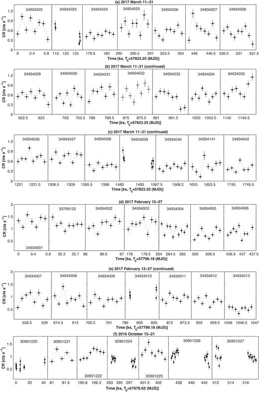
The 0.3–10 keV light curves from the most densely sampled XRT observations of OJ 287 during 2016 April–2017 June.
The source showed seven 0.3–10 keV IDVs during the XRT campaign in 2017 February 15–27 (ObsIDs (3493400)2–8, panels 3–7 of Fig. 4(d) and panels 1 and 2 of Fig. 4e) which were observed within the exposures ≲1 ks. However, they showed lower fractional amplitudes than those recorded during the aforementioned campaign (Fvar = 14.7(3.9)–23.9(4.8)) and narrower ranges of the spectral parameters (Γ = 2.30(0.08)–2.75(0.07), and HR = 0.22(0.03)–0.47(0.06)). Two IDVs occurring within 1 ks intervals were observed during the campaign of 2016 October 15–21 (ObsID 30901221 and the first orbit of ObsID 30901227, panels 2 and 7 of Fig. 4f, respectively).
Other interesting 0.3–10 keV IDVs, mostly occurring within 1 ks exposures are presented in Fig. 5. However, the instances, provided in the bottom row, were characterized by relatively large background which was comparable to the count rates corresponding to the minima of light curves (amounting to 60–80 per cent of the background-subtracted signal). Therefore, these IDVs should be treated with caution.
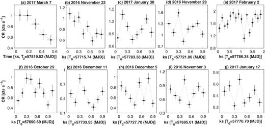
Other very fast 0.3–10 keV IDVs in OJ 287 during 2016 April–2017 June.
OJ 287 showed eleven 0.3–0 keV IDVs at the 99.5 per cent confidence level (so-called possible variability, Andruchow, Romero & Cellone 2005; see Table 6). Note that the majority of these instances belong to the epochs of the intensive XRT campaigns performed during 2016 October 15–21 and 2016 March 11–31 (discussed above). Finally, nine instances of optical–UV IDVs were detected at the 99.5 and 99.9 per cent confidence levels with UVOT, characterized by Fvar = 7.3(1.9)–16.6(1.6) per cent (see Table 7).
Summary of the optical–UV IDVs in 2016 April–2017 June.
| ObsID(s) | Obs. start (MJD) | Obs. end (MJD) | Band | |$\chi ^2_{\rm r}$|/d.o.f. | Fvar(percent) | Δm |
|---|---|---|---|---|---|---|
| 99.9 (per cent) | ||||||
| 30901244–30901245 | 57703.841 | 57704.771 | B | 11.65/1 | 7.5(1.5) | 0.12(0.04) |
| 34934034–34934035 | 57835.202 | 57836.199 | UVM2 | 55.23/1 | 16.6(1.6) | 0.26(0.05) |
| 34934034–34934035 | 57835.197 | 57836.194 | UVW2 | 14.59/1 | 15.1(2.9) | 0.24(0.05) |
| 34934035–34934036 | 57836.199 | 57837.137 | UVW2 | 21.05/1 | 12.0(1.9) | 0.20(0.05) |
| 34934035–34934036 | 57836.193 | 57837.131 | UVW2 | 13.35/1 | 14.5(3.0) | 0.23(0.05) |
| 99.5 (per cent) | ||||||
| 30901226–30901227 | 57281.252 | 57682.115 | V | 8.94/1 | 7.3(1.9) | 0.12(0.04) |
| 34934034–34934035 | 57835.201 | 57836.198 | B | 9.32/1 | 9.2(2.3) | 0.15(0.05) |
| 30901226–30901227 | 57281.253 | 57682.116 | B | 10.06/1 | 7.4(1.8) | 0.12(0.05) |
| 34934040–34934041 | 57841.189 | 57841.177 | UVM2 | 10.23/1 | 7.5(1.8) | 0.12(0.05) |
4 RESULTS FROM THE SPECTRAL ANALYSIS
We performed the 0.3–10 keV spectral analysis using the xspec package included in heasoft. For this purpose, the latest response matrix from the XRT calibration files from Swift CALDB and ARFs were adopted. The latter were generated by means of the XRTMKARF task to account for the PSF losses, different extraction regions, vignetting, and CCD defects. The instrumental channels were combined to include at least 20 photons per bin by means of the ftools task GRPPHA (enabling the use of χ2-statistics). However, in the case of the low X-ray state of the source and short exposure, the corresponding spectrum was very poor and we did not group channels in order to use Cash statistics.
For themajority of the spectra (103 out of 132), a simple power law was clearly preferred by the aforementioned tests. The corresponding results (the values of different spectral parameters, de-absorbed 0.3–2, 2–10, 0.3–10 keV fluxes, and hardness ratio) are provided in Table 8. The hardness ratio was calculated as HR = |$F_{\rm 2-10\, keV}/F_{\rm 0.3-2\, keV}$| where the symbols |$F_{\rm 2-10\, keV}$| and |$F_{\rm 0.3-2\, keV}$| denote the de-absorbed 2–10 to 0.3–2 keV fluxes, respectively.
The results of the XRT spectral analysis with a simple power-law model (extract). In column (4), an asterisk stands for the parameter Goodness (in per cents) when the Cash statistics was applicable. The de-absorbed 0.3–2, 2–10, and 0.3–10 keV fluxes (columns 5–7) are given in 10−12 erg cm−2 s−1.
| ObsId | Γ | 1000× K | |$\chi ^2_{\rm r}$|/d.o.f. | |$F_{\rm 0.3-2\, keV}$| | |$F_{\rm 2-10\, keV}$| | |$F_{\rm 0.3-10\, keV}$| | HR |
|---|---|---|---|---|---|---|---|
| (1) | (2) | (3) | (4) | (5) | (6) | (7) | (8) |
| 30901209 | 2.84(0.32) | 0.62(0.22) | 55.6* | 2.61(0.46) | 0.42(0.18) | 3.10(0.57) | 0.16(0.07) |
| 30901210 | 2.41(0.23) | 0.85(0.23) | 59.8* | 3.57(0.48) | 1.51(0.56) | 5.02(0.85) | 0.42(0.18) |
| 30901212 | 2.44(0.30) | 0.8(0.14) | 57.2* | 2.80(0.42) | 1.09(0.43) | 3.88(0.59) | 0.39(0.18) |
| 30901213 | 2.5(0.35) | 0.80(0.14) | 55.3* | 3.09(0.49) | 1.02(0.57) | 4.11(0.76) | 0.33(0.16) |
| 30901214 | 2.65(0.34) | 1.05(0.19) | 58.7* | 4.01(0.67) | 1.05(0.44) | 5.08(0.76) | 0.26(0.13) |
| 30901215 | 2.29(0.27) | 1.03(0.20) | 43.8* | 3.96(0.49) | 1.45(0.47) | 5.61(0.92) | 0.37(0.15) |
| 30901217 | 2.46(0.15) | 1.68(0.13) | 0.866/4 | 5.35(0.53) | 2.77(0.59) | 8.12(1.36) | 0.52(0.13) |
| 30901219 | 2.63(0.06) | 6.19(0.22) | 0.924/33 | 23.50(0.96) | 6.46(0.57) | 29.92(0.35) | 0.27(0.03) |
The photon index Γ showed a wide range of ΔΓ = 1.0 with the hardest value Γmin = 1.90 ± 0.14 (see Fig. 6a and Table 9). On average, the spectra were the hardest in interval 6 with a mean value of the photon index |$\overline{\Gamma }$| = 2.06, while the softest spectra with |$\overline{\Gamma }$| = 2.73 were recorded in interval 2. This parameter showed a weak positive correlation with the de-absorbed 0.3–10 keV flux (see Fig. 7a, as well as Table 10 for the Spearman correlation and the corresponding p-chance). This result implies that the source mainly followed a ‘softer-when-brighter’ spectral trend in the here-presented period. In fact, the lowest values of the photon index belong to interval 6 when the source showed its lower 0.3–10 keV states, while the largest mean value of the parameter Γ was observed in interval 2 when OJ 287 was showing an X-ray outburst. This trend is also evident from Figs 8(a) and (b) where the de-absorbed 0.3–10 keV flux and the parameter Γ are plotted as functions oftime.
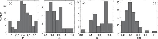
Distribution of the values of spectral parameters.
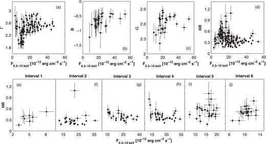
Correlation between the spectral parameters and de-absorbed 0.3–10 keV flux.
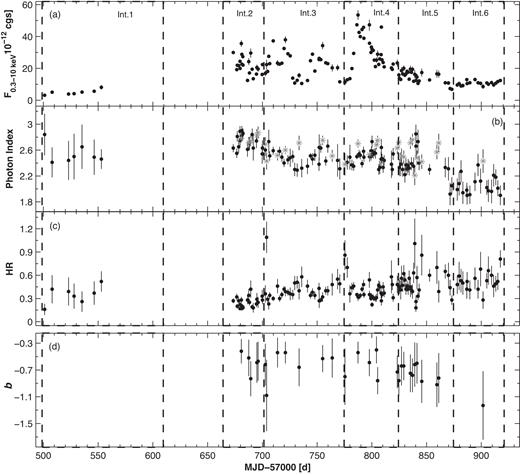
Unabsorbed 0.3–10 keV flux (top panel), photon index (panel b), hardness ratio (panel c), and curvature parameter in 2016 April–2017 June as a function of time. In panel (a), the acronym ‘cgs’ denotes erg cm−2s−1. The vertical dashed lines indicate the periods discussed in Section 3.2.
Distribution of spectral parameters in different periods.
| Quantity | Min. value | Max. value | Mean value | Skewness |
|---|---|---|---|---|
| Γ | 1.90 | 2.90 | 2.44 | −0.37 |
| a | 2.21 | 2.87 | 2.61 | −0.58 |
| b | −1.23 | −0.40 | −0.68 | −0.76 |
| HR | 0.16 | 1.09 | 0.41 | 1.28 |
| Quantity | Min. value | Max. value | Mean value | Skewness |
|---|---|---|---|---|
| Γ | 1.90 | 2.90 | 2.44 | −0.37 |
| a | 2.21 | 2.87 | 2.61 | −0.58 |
| b | −1.23 | −0.40 | −0.68 | −0.76 |
| HR | 0.16 | 1.09 | 0.41 | 1.28 |
Correlations between the spectral parameters and multiband fluxes (denoted by ‘Fi’ for the particular i-band).
| Quantities | r | p |
|---|---|---|
| Γ and |$F_{\rm 0.3-10\, keV}$| | 0.37(0.11) | 2.44 × 10⁻⁵ |
| a and |$F_{\rm 0.3-10\, keV}$| | 0.33(0.20) | 0.046 |
| b and |$F_{\rm 0.3-10\, keV}$| | 0.40(0.11) | 8.10 × 10⁻⁴ |
| HR and |$F_{\rm 0.3-10\, keV}$| | −0.29(0.05) | 5.03 × 10⁻³ |
| HR and |$F_{\rm 0.3-10\, keV}$| (Int. 3) | −0.43(0.08) | 1.29 × 10⁻⁶ |
| |$F_{\rm 0.3-2\, keV}$| and |$F_{\rm 2-10\, keV}$| | 0.69(0.06) | 2.48 × 10⁻¹¹ |
| |$F_{\rm 0.3-10 \, keV}$| and FUVW2 | 0.63(0.07) | 3.32 × 10⁻¹⁰ |
| |$F_{\rm 0.3-10 \, keV}$| and FB | 0.62(0.07) | 7.67 × 10⁻¹⁰ |
| |$F_{\rm 0.3-10 \, keV}$| and FR | 0.57(0.08) | 6.41 × 10⁻⁹ |
| |$F_{\rm 0.3-10 \, keV}$| and FJ | 0.50(0.10) | 4.90 × 10⁻⁸ |
| FUVW2 and FUVM2 | 0.97(0.01) | <10−15 |
| FUVW2 and FU | 0.88(0.02) | <10−15 |
| FUVW2 and FV | 0.90(0.02) | <10−15 |
| FB and FV | 0.96(0.01) | <10−15 |
| V − UVW1 and UVW1 | −0.46(0.09) | 3.06 × 10⁻⁷ |
| V − UVW2 and UVW2 | −0.43(0.10) | 6.64 × 10⁻⁶ |
The latter figure also shows that the photon index varied on different time-scales. The largest variability was recorded in interval 5 (a hardening by ΔΓ = 0.93 ± 0.22 during MJD 57840.3–57871.5). On intraday time-scales, this parameter was variable only once: a softening by ΔΓ = 0.26 ± 0.10 during MJD 57676.6–57677.1).
On 29 occasions, the spectrum demonstrated a good fit with the log-parabola model which was related to the presence of an upward curvature (i.e. a negative value of the parameter b) with Δb = 0.83 and bmin = −1.23 ± 0.51 (see Fig. 6b and Table 9 for the distribution of the curvature parameter). Table 11 presents the corresponding results (the values of different spectral parameters, de-absorbed 0.3–2, 2–10, 0.3–10 keV fluxes, and hardness ratio for each curved spectrum). The 0.3–10 keV SEDs of two log-parabolic spectra (corresponding to smaller and larger curvatures) are provided in Fig. 9. In this figure, we also have provided plots presenting a power-law fit for the same spectra, demonstrating clear trends in the distribution of the fit residuals with energy, which are not present when adopting the log-parabola model.
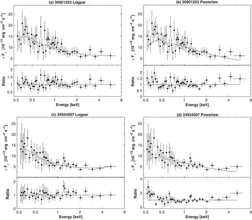
The 0.3–10 keV SEDs of two spectra well fitted with the log-parabola model with the curvatures b = −0.44 ± 0.16 (panel a) and b = −0.86 ± 0.20 (panel b). For a comparison, panels (c) and (d) present a power-law fit with the same spectra.
Results of the spectral analysis with the log-parabola model. The de-absorbed 0.3–2, 2–10, and 0.3–10 keV fluxes (columns 6–8) are given in 10−12 erg cm−2s−1.
| ObsId | a | b | 100× K | χ2/d.o.f. | |$F_{\rm 0.3-2\, keV}$| | |$F_{\rm 2-10\, keV}$| | |$F_{\rm 0.3-10\, keV}$| | HR |
|---|---|---|---|---|---|---|---|---|
| (1) | (2) | (3) | (4) | (5) | (6) | (7) | (8) | (9) |
| 30901225 | 2.78(0.06) | −0.42(0.18) | 6.30(0.32) | 0.918/41 | 27.73(1.43) | 7.89(1.07) | 35.56(1.99) | 0.28(0.04) |
| 30901229 | 2.71(0.09) | −0.52(0.27) | 4.01(0.27) | 0.860/23 | 18.11(1.36) | 6.10(1.25) | 24.21(2.08) | 0.34(0.07) |
| 30901131 | 2.74(0.08) | −0.83(0.26) | 4.20(0.29) | 0.930/22 | 20.89(1.44) | 8.67(1.99) | 29.58(2.79) | 0.42(0.09) |
| 30901137 | 2.83(0.09) | −0.59(0.30) | 3.43(0.24) | 0.995/24 | 15.92(1.03) | 4.56(1.04) | 20.51(1.76) | 0.29(0.06) |
| 30901138 | 2.87(0.09) | −0.57(0.29) | 3.18(0.22) | 1.149/28 | 15.74(1.19) | 3.88(0.92) | 19.63(1.72) | 0.25(0.05) |
| 30901143 | 2.69(0.11) | −0.62(0.31) | 2.71(0.33) | 0.910/14 | 12.42(1.17) | 4.46(1.08) | 16.87(1.77) | 0.36(0.08) |
| 30901144 | 2.43(0.13) | −1.08(0.47) | 2.45(0.24) | 0.961/16 | 10.72(0.99) | 11.64(3.49) | 22.34(3.02) | 1.09(0.17) |
| 30901149 | 2.52(0.08) | −0.44(0.22) | 3.95(0.21) | 0.845/27 | 16.00(1.07) | 7.31(1.24) | 23.28(1.80) | 0.46(0.07) |
| 30901153 | 2.60(0.06) | −0.44(0.16) | 6.45(0.27) | 0.949/47 | 27.23(1.34) | 10.69(1.38) | 37.93(2.12) | 0.39(0.05) |
| 33756093 | 2.71(0.11) | −0.66(0.28) | 2.35(0.24) | 0.953/22 | 11.14(1.00) | 4.43(1.04) | 15.60(1.51) | 0.40(0.08) |
| 33756101 | 2.75(0.07) | −0.53(0.20) | 5.60(0.31) | 1.027/43 | 26.00(1.51) | 8.24(1.35) | 34.28(2.22) | 0.32(0.04) |
| 33756105 | 2.51(0.09) | −0.52(0.29) | 3.36(0.23) | 1.097/23 | 13.74(1.03) | 6.61(1.58) | 20.32(2.16) | 0.48(0.10) |
| 33756109 | 2.38(0.17) | −0.80(0.42) | 1.48(0.21) | 1.098/12 | 6.07(0.78) | 5.20(1.84) | 11.27(1.79) | 0.86(0.18) |
| 33756115 | 2.70(0.06) | −0.44(0.16) | 9.10(0.38) | 0.856/58 | 40.46(2.00) | 12.91(1.67) | 53.46(2.88) | 0.32(0.04) |
| 33756121 Orbit 1 | 2.53(0.07) | −0.59(0.20) | 7.50(0.48) | 0.906/25 | 30.76(1.79) | 16.60(2.70) | 47.32(3.57) | 0.54(0.08) |
| 34934006 | 2.68(0.07) | −0.40(0.20) | 4.45(0.24) | 1.118/38 | 19.19(1.16) | 5.98(0.90) | 25.18(1.58) | 0.31(0.04) |
| 34934007 | 2.75(0.07) | −0.86(0.20) | 4.03(0.23) | 1.075/38 | 20.46(1.37) | 8.43(1.43) | 28.91(2.18) | 0.41(0.05) |
| 34934022 | 2.63(0.09) | −0.73(0.24) | 3.44(0.24) | 0.945/30 | 15.74(1.22) | 7.59(1.50) | 23.33(2.15) | 0.48(0.08) |
| 34934023 | 2.72(0.09) | −0.86(0.23) | 2.35(0.23) | 1.104/16 | 10.89(0.77) | 4.98(0.89) | 15.85(1.29) | 0.46(0.08) |
| 34934026 | 2.51(0.11) | −0.64(0.29) | 2.82(0.24) | 1.159/23 | 11.94(1.10) | 6.65(1.54) | 18.58(2.14) | 0.56(0.08) |
| 34934028 | 2.49(0.10) | −0.64(0.21) | 3.04(0.24) | 0.905/26 | 12.36(0.96) | 7.62(1.18) | 20.00(1.68) | 0.62(0.07) |
| 34934034 | 2.71(0.09) | −0.75(0.28) | 2.87(0.22) | 0.946/22 | 13.43(1.07) | 6.07(1.43) | 19.50(2.08) | 0.45(0.08) |
| 34934036 | 2.76(0.09) | −0.78(0.25) | 2.87(0.22) | 0.955/23 | 13.84(1.04) | 5.46(1.05) | 19.32(1.66) | 0.39(0.07) |
| 34934038 | 2.21(0.15) | −0.62(0.33) | 2.18(0.24) | 1.090/16 | 8.05(0.94) | 8.17(2.04) | 16.22(2.51) | 1.01(0.21) |
| 34934040 | 2.48(0.11) | −0.60(0.30) | 2.23(0.24) | 1.138/16 | 9.20(0.87) | 5.28(1.13) | 14.49(1.61) | 0.57(0.11) |
| 34934043 | 2.42(0.11) | −0.87(0.32) | 2.20(0.24) | 1.023/14 | 9.35(0.96) | 8.02(1.96) | 17.38(2.42) | 0.86(0.16) |
| 34934045 | 2.57(0.11) | −0.92(0.33) | 2.15(0.23) | 0.917/21 | 9.73(1.00) | 6.84(1.68) | 16.56(2.40) | 0.70(0.14) |
| 34934046 | 2.71(0.14) | −0.82(0.37) | 2.45(0.28) | 1.012/12 | 11.78(1.38) | 4.54(1.27) | 16.33(2.17) | 0.39(0.10) |
| 34934063 | 2.43(0.18) | −1.23(0.51) | 1.34(0.23) | 0.973/8 | 6.70(0.73) | 1.88(0.58) | 8.58(1.45) | 0.28(0.09) |
Curved spectra are found for XRT observations performed during intervals 2–6, in different brightness states of the source and the parameter b exhibited a weak positive correlation with the 0.3–10 keV flux (see Fig. 7b and Table 10). Due to the relatively large uncertainties, the parameter b did not show variability on short time-scales (Fig. 8d).
The curved spectra showed a range of photon index at 1 keV Δa = 0.66 with the hardest value amin = 2.21 ± 0.15 (Fig. 6c and Table 9). This parameter underwent the largest and fastest variability with Δa = 0.55 ± 0.17 (a hardening, during MJD 57837.1–57839.2; Fig. 8b). Similar to the 0.3–10 keV photon index, the parameter a also showed a weak positive correlation with the X-ray brightness, although the spectra from the highest states did not follow a ‘softer-when-brighter’ trend (see Fig. 7c).
The hardness ratio, derived from both power-law and log-parabolic spectra, was characterized by a very wide range of values ΔHR = 0.93 and two occasions of HR >1, associated with the curved spectra. This parameter varied on different time-scales with the largest shift by 0.91 to higher values in 12 d (MJD 57691.8–57703.8) and showed the presence of the ‘softer-when-brighter’ evolution (Fig. 7d). However, the weakness of the correlation and a large deviation of some data points from the general trend indicate that the source did not always follow this trend in the 2016 April–2017 June period. Namely, it showed an HR–F0.3-10keV anticorrelation at the 99 per cent confidence level only in interval 3 (Fig. 7g). This trend dominated also in interval 4, although the data points, corresponding to the highest X-ray states, do not follow it and the correlation was below the aforementioned confidence (Fig. 7h). On the contrary, the data points from intervals 1 and 6 show the opposite trend, although below the 99 per cent confidence level, and no clear trend was evident during intervals 2 and 5 (Figs 7f and i, respectively).
5 DISCUSSION AND CONCLUSIONS
5.1 Flux variability
During the extensive XRT observations in 2016 October–2017 April, OJ 287 showed unprecedented X-ray flaring activity, expected in the framework of the propagation of a strong shock in the inner (subparsec) jet after the second impact of the secondary BH on the accretion disc of the primary one. However, no strong X-ray activity was evident along with the strong optical–UV outbursts observed in 2015 December–2016 May (possibly owing to the first impact), 2005–2006, and 1994–1996 (previous close encounters of the primary and secondary BHs). Such a behaviour can be explained by the absence of X-ray emission on parsec-scale distances from the jet base which is resolvable by VLBA observations and showing possible precession and nutation with ∼22 and ∼1 yr periods, respectively (causing the low-energy variability; Britzen et al. 2018). A stronger X-ray flaring activity in 2016 October–2017 April could be related to the propagation of a relativistic shock through the subparsec jet which was considerably stronger than those triggered by the first impact causing an optical–UV outburst, or those related to the previous BH encounters, triggering the outbursts in 1994–1996 and 2005–2006. The propagation of a stronger shock could yield the acceleration of a much higher number of electrons to the energies sufficient to generate 0.3–10 keV photons by means of the first-order Fermi mechanism at the shock front (Massaro et al. 2004), or via the stochastic processes related to the jet turbulence strongly amplified after the shock passage (see Tramacere, Massaro & Taylor 2011; Mizuno et al. 2014). The same electrons were able to emit also at the optical–UV frequencies and this possibility is confirmed by the observed positive correlation between the XRT and UVOT-band fluxes (see Section 5.3) which was not the case during the previous optical outbursts.
As an LBL/IBL object, OJ 287 generally was a faint X-ray source before 2016 October. It was observed with the satellite Einstein (1979–1980, Madejski & Schwartz 1988), EXOSAT (1983–1984, Sambruna et al. 1994), and ROSAT (1991, Comastri, Molendi & Ghisellini 1995), exhibiting steep X-ray spectra and brightness variation by a factor of 3 on the time-scales of months and by 30 per cent within 3 d. However, the Ginga observations, performed in 1989–1990, failed to detect X-rays from this object (Urry et al. 1996). The ASCA pointings in 1997 April and November yielded a 0.5–10 keV flux lower than that obtained in previous X-ray campaigns, and no evidence of intensity variations was found during each observation (Isobe et al. 2001). The Swift-XRT monitoring in 2005 May–2016 May showed flares by a factor of 2–4 on weekly time-scales, although the mean 0.3–10 keV count rate was 0.20 versus 0.93 counts s−1 during intervals 2–5 discussed in Section 3.2. The shortest variability time-scale was ∼1 d, strongly limited by the pointing of the observations (Siejkowski & Wierzcholska 2017). During the optical outburst in 2015 December, an X-ray flare was rather modest, much smaller than the optical one and did not differ significantly from those X-ray flares observed during the campaigns of the previous 12 months (Valtonen et al. 2016).
We obtained a range of de-absorbed 2–10 keV fluxes between 4.30 × 10⁻¹³ and 1.30 × 10⁻¹¹ erg cm−2s−1. This range is wider than those reported by Siejkowski & Wierzcholska (2017): (1.0–11.8) × 10−11 erg cm−2s−1 (the XRT monitoring during 2005 May–2016 May), or derived from observations with other X-ray space missions: (1.42–2.68) × 10−11 erg cm−2s−1 in the case of the XMM–Newton pointings during 2005 April–November (Raiteri et al. 2007); (1.44–3.42) × 10−11 erg cm−2s−1 from the Suzaku pointings in 2007 April and November (Seta et al. 2009).
The soft 0.3–2 keV flux showed a range (0.26–4.05) × 10−11 erg cm−2s−1. Note that the mean 0.3–2 keV flux during the outburst epoch (intervals 2–5) increased by a factor of 2.7 compared to the mean flux from intervals 1 and 6 (the epochs of a relative quiescence), while the same ratio was only 1.9 in the hard 2–10 keV band. We conclude that the soft X-ray photons made more contribution to the observed X-ray outburst than those from the hard X-ray range.
The Γ–flux, a–flux, and HR–flux planes showed a dominance of a ‘softer-when-brighter’ spectral evolution of the source, which can be explained by the consecutive emergence of soft X-ray components in the X-ray emission zone, resulting in the brightness increase but softening the observed 0.3–10 keV spectrum (see e.g. Kapanadze et al. 2018b). Contrary to this, the source showed a ‘harder-when-brighter’ trend during 2005 May–2016 May when no strong X-ray outburst was observed (Siejkowski & Wierzcholska2017).
In Fig. 10(a), we plot the Fvar values, calculated using equation (4) from the observations of OJ 287 performed with XRT, UVOT, LAT, and ground-based optical–radio telescopes in the 2016 October–2017 April period, as a function of frequency. For this purpose, the daily-binned radio–X-ray datawere used. Since almost half of the weekly binned LAT data yielded a detection of the source below a 3σ significance or the parameter Npred was less than 10, we used two-weekly binned data to calculate the quantity Fvar. Moreover, the HE emission of our target was concentrated in the 0.1–2 GeV band, while the source generally was detectable only below 3σ significance or showed Npred <10 in the 2–300 GeV energy range even in the case of two-weekly binned data. Therefore, the LAT data point in Fig. 10 was calculated only for the 0.1–2 GeV emission. We see that the variability power, presented by Fvar, was becoming gradually stronger with increasing energy and peaking at softX-rays.
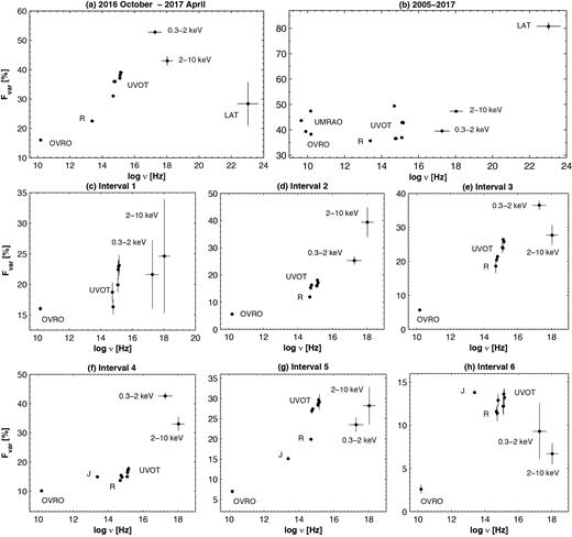
Fractional variability amplitude as a function of frequency in different periods.
However, the Fvar–frequency plane, constructed for the period 2005–2017 (excluding the data obtained during 2016 October–2017 April), demonstrates a different situation (see Fig. 10b): the highest value of Fvar is shown in γ-rays, and the source showed the strongest variability at synchrotron frequencies in the case of the R-band observations performed with different ground-based optical telescopes. However, the corresponding data are significantly more densely sampled than those obtained with UVOT and XRT in the same period, and this result should be treated with caution. Note that the source showed a considerably stronger radio variability in this period than during 2016 October–2017 April: the UMRAO 4.5–14.5 GHz and OVRO 15 GHz observations yielded Fvar = 38.3–47.4 per cent during 2005–2017, while Fvar = 16.0 per cent in the case of the OVRO observations in the latter period.
The middle and bottom rows of Fig. 10 present the Fvar–energy plane constructed for the intervals discussed in Section 3.2 in the radio–X-ray energy range. In interval 1, the Fvar value does not show significant variability in the 2–10 keV band, and the strongest variability was recorded at UV frequencies (Fig. 10c). In intervals 2–4, the source showed maximum values of Fvar in the 0.3–2 and 2–10 keV bands, significantly exceeding those in the lower energy ranges (Figs 10d–f). However, the X-ray variability power was already lower in interval 5: the maximum of Fvar shifted towards lower frequencies, and this quantity was seen in the IR–UV range in interval 6 (Figs 10g and h, respectively). However, a high J-band value in interval 6 could be related to sparsely sampled data and it should be treated with caution.
During intervals 2–5, the source showed enhanced X-ray activity also on intraday time-scales. The duty cycle (DC, i.e. the fraction of total observation time during which the object displays variability; Romero et al. 1999), corresponding to 32 X-ray IDVs detected at the 99.9 per cent confidence within our study, amounts to 26.7 per cent which is comparable to the DC of the 0.3–10 keV IDVs shown by the HBL source 1ES 1959 + 650 during the XRT observations in 2005–2016 (Kapanadze et al. 2016a,b). Note that the 0.3–10 keV variability of OJ 287 during 2016 October–2017 April was characterized by the highest level of the X-ray activity of an LBL/IBL source on intraday time-scales, reported to date.
The fractional variability amplitudes of the IDVs show an anticorrelation with the 0.3-10 keV flux, yielding the Spearman correlation coefficient ρ = 0.73 ± 0.08 (Fig. 11). The highest value Fvar = 59.7 ± 5.8 per cent was derived from ObsID 34934023 (MJD 57824.7; the second panel of Fig. 4a) when the orbit-binned count rate dropped by a factor of 2.4 in 13 ks. The corresponding 0.3–10 keV flux slightly exceeded the mean flux during 2005–2017 (denoted by vertical dashed line in Fig. 11). On the contrary, the IDVs with Fvar <15 per cent correspond to flux values (2.5–4.7) × 10−11 erg cm−2s−1 which are factors of 2.2–4.1 higher than the mean flux during 2005–2017 period. Note that an anticorrelation between fractional amplitude and flux was also reported by Zhang et al. (2006) and Kapanadze et al. (2016a) for PKS 2155 − 304 and 1ES 1959 + 650, respectively, that was suggested to be an indication of a strong non-stationary origin of the X-ray variability.
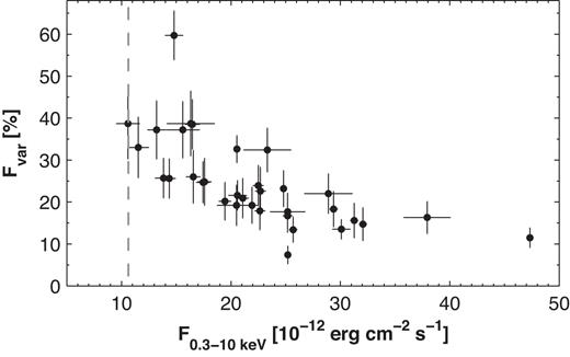
Fractional variability amplitude of the X-ray IDVs detected with a 99.9 per cent confidence level as a function of the XRT flux. A vertical, dashed grey line shows the weighted mean 0.3–10 keV flux during 2005–2017.
Moreover, Fig. 11 demonstrates that X-ray IDVs in OJ 287 generally occurred during the higher brightness states in the here-presented period which favours a shock-in-jet scenario (interaction of a propagating shock front with jet inhomogeneities; Sokolov, Marscher & McHardy 2004; Kapanadze et al. 2018a). The IDVs triggered by other mechanisms, acting in the innermost blazar zone, should be more conspicuous in low states when the variable emission from the this zone is not ‘shadowed’ by that produced at the front of the shock front which is propagating through the jet. We have not found 0.3–10 keV IDVs in the lower states of OJ 287 observed during intervals 1 and 6, and a similar result was reported by Siejkowski & Wierzcholska (2017) for the XRT observations performed during 2005–2016 when the source did not show X-ray outbursts. Isobe et al. (2001) also failed to find X-ray IDV during the ASCA observations of our target performed in 1997. No X-ray activity on intraday time-scales was reported from the BeppoSAX observations in 2001 November (Massaro et al. 2003) or from the 2005 April observations with XMM–Newton (Massaro et al.2008).
In the present study, we detected one optical (B band) and four UV (UVW2 band) IDVs from UVOT observations of OJ 287. From past observations, optical R-band IDVs from six nights were reported from observations performed in 2015 December–2016 May, while no V-band IDVs were detected in the same period (Gupta et al. 2017). Rakshit et al. (2017) found the source variable during six nights (out of 21) with the fastest time-scale of 142 ± 38 min in the R band during 2015 December–2016 February. Intraday variation time-scales of 10 min to 2 h were detected in the V, R, and I bands (four, seven, and nine instances, respectively) by Fan et al. (2009) in the period 2002–2007. However, no information about the variability detection tests are provided, and we cannot exclude the influence of the variable seeing conditions during these instances. No IDV was detected during the four nights of the R-band observations in 2006 October–2007 January (Gupta et al. 2008).
5.2 The ranges and variability of spectral parameters
The majority of the 0.3–10 keV spectra of OJ 287 were fitted well with a simple power law during the here-presented period, yielding the photon index Γ = 1.90–2.90. Siejkowski & Wierzcholska (2017) fitted all the XRT-band spectra, derived from observations of OJ 287 in 2005 May–2016 May, with a simple power law and obtained a very wide range of values of the photon index Γ = 1.19–2.43. Note that a number of these values are considerably harder than the hardest value of the photon index obtained within our study. Especially hard values were derived during their time intervals A and B (MJD 53510–54917, 2005 May–2009 March) with the mean values |$\overline{\Gamma }$| = 1.49–1.59, and this result can be explained as due to the pure IC origin of the 0.3–10 keV emission in an LBL-/IBL-type source (see Isobe et al. 2001). However, the corresponding spectra generally were very poor due to X-ray faintness of the source and short exposures. Therefore, it is impossible to draw a conclusion about the better fit with the log-parabola model compared to the power law and detect an upward curvature (if any exists). However, the authors constructed broad-band optical–X-ray SEDs for each interval and obtained a spectral upturn from the optical–UV to the X-ray component (similar to other time intervals in the subsequent years). Note that we met a similar situation with the spectra from interval 6: the photon index was the hardest during the entire here-presented period, although very poor spectra (yielding 4–8 degrees of freedom, or those fitted with the Cash statistics) allowed us to detect a spectral curvature only for one spectrum. Re-analysing the spectra presented in Siejkowski & Wierzcholska (2017), a significant upward curvature was detected by Gaur et al. (2018) for those extracted from the observations performed on MJD 53677, 54056, and 55849, with a break energy in the 1.5–3.0 keV range.
Due to the long-term high X-ray state of OJ 287 in 2016 October–2017 April, we were able to extract considerably richer 0.3–10 keV spectra of our target and detect an upward curvature on29 occasions. They exhibited a wide range of the curvature parameter and more than 90 per cent of the values were included in the interval (−0.4, −0.9). Along with the better statistics in the case of the log-parabolic fit for these spectra, they show prominent trends in the fit residuals when adopting a power-law fit (see Fig. 9). An IC contribution to the 0.3–10 keV spectrum was reported even for the HBL source PKS 2155 − 304 by Zhang (2008) from XMM–Newton observations performed in lower X-ray states. Moreover, the study of the broad-band SEDs of OJ 287 in the UVOT–XRT energy range by Kushwaha et al. (2018a) during the here-presented period confirmed the presence of different spectral components at X-ray frequencies.
The log-parabolic spectra of OJ 287 generally showed very steep photon index at 1 keV (more than 90 per cent of them showing Γ >2.4), allowing the IC emission to make a significant contribution in the 0.3–0 keV energy range. Steep or very steep values of the photon index were derived from the spectra belonging to intervals 2–5, although the elevated X-ray flux and, on average, one of the lowest 0.1–30 GeV states of OJ 287 since the start of Fermi operations yielded insignificant IC contribution and an absence of upward curvature.
Note that the presence of two different spectral components in the X-ray energy range is common to the LBL/IBL sources. For example, the presence of an upward curvature was reported for five objects (3C 66A, S5 0716 + 714, W Comae, 4C+21.35, and BL Lacs; Wierzcholska & Wagner 2016), permitting simultaneous, time-resolved studies of both ends of the electron distribution. The analysis of multi-epoch observations revealed that the break energy varies only by a small factor with flux changes. Flux variability was more pronounced in the synchrotron domain (HE end of the electron distribution) than in the Compton domain (low-energy end of the electron distribution) in these sources. The presence of both synchrotron and IC components in the 0.5–10 keV spectrum of OJ 287 was suggested by Idesawa et al. (1997) from ASCA observations of the source performed in 1994 November, and their fit with a simple power law yielded a hard value of the photon index (Γ ∼1.70) in that epoch. The latter ASCA observations (1997 April and November) yielded flatter power-law spectra with Γ = 1.5–1.6, leading Isobe et al. (2001) to the suggestion that these spectra should arise via the IC process alone.
The BeppoSAX observations in 2001 November showed that the simple power-law extrapolations of the optical data into the X-ray range yields higher flux values than the measured fluxes, and this problem is solved via the assumption that the broad-band emission contains two different components (Massaro et al. 2003). The presence of the IC component in the X-ray emission of OJ 287 was reported also from the Swift-XRT and XMM–Newton observations of OJ 287 in 2005 April–May (Massaro et al. 2008).
From the Suzaku observations of our target in 2007 April and November, Smith et al. (2009) reported a fit of the 0.5–10 keV spectra with a simple power law yielding Γ = 1.50–1.65. However, the observation in a lower X-ray state showed a trend in the fit residuals at higher energies, possibly related to an IC contribution.
5.3 MWL correlations
Fig. 12(a) demonstrates a positive correlation between the de-absorbed soft 0.3–2 keV and hard 2–10 keV fluxes from the XRT observations of OJ 287 performed in the period 2016 April–2017 June. Note that the HBL sources have shown significantly stronger |$F_{\rm 0.3-2 \, keV}$|–|$F_{\rm 0.2-10 \, keV}$| correlation in different periods (see e.g. Kapanadze et al. 2014, 2016c, 2017, 2018a), confirming the origin of the soft and hard X-ray emissions from the same jet electron population, produced via the synchrotron mechanism. A lower strength of this correlation in OJ 287 can be explained by the generation of the X-ray photons by both synchrotron and IC mechanisms, reflected in the spectral curvature during some XRT observations. Note also that the majority of the data points, corresponding to the log-parabolic spectra (grey asterisks) with relatively low upward curvature, follow a general trend in Fig. 12(a) and indicate a comparable contribution of IC photons in both 0.3–2 and 2–10 keV bands. However, the data points from the spectra with higher curvature produce outliers from the scatter plot, indicating the major contribution of the IC photons to the hard X-ray energy range.
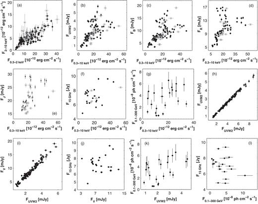
Correlations between multiband fluxes. In panels (a)–(f), the grey asterisks correspond to the data derived from the log-parabolic spectra.
During intervals 3–5 (the period of X-ray outburst), the source showed stronger flaring activity in the 0.3–2 keV band (see Table 5 for the values of the corresponding Fvar), while a stronger variability was observed at hard X-ray frequencies in interval 2.19 This difference was reflected in the spectral variability (discussed in Section 4), which can lead to the appearance of the clockwise (CW) or counterclockwise (CCW) ‘loops’ in the HR–flux plane. These features can indicate different interplay between the acceleration (τacc) and synchrotron cooling (τsyn) time-scales of the X-ray emitting particles and flux variability time-scale (τvar; see e.g. Cui 2004; Falcone et al. 2004; Kapanadze et al. 2018a), which can be related as (i) τsyn ≫ τvar ≫ τacc, or τsyn ≫ τacc ≫ τvar in the case of the CW-type evolution; (ii) τsyn ≈ τacc ≈ τvar when the source shows a CCW-type loop. In the former case, a rapid injection of very energetic particles in the emission zone should cause the appearance of a new flaring component starting in the hard X-ray band, making the spectrum progressively harder in the brightening phase of the source and softer during the declining one. Therefore, the flux variability in the hard X-ray range leads that of the soft X-rays during the flaring and declining phases, and a soft lag is expected. In the case of the CCW-type evolution, the particles are gradually accelerated, with the flare at soft X-rays leading that at higher energies and the brightness decline epoch can be dominated by particle escape effects. Consequently, a hard lag during the X-ray flare is expected (Falcone et al. 2004). Figs 13(b), (d), (f), (g), (i), (j), (l), and (m) (corresponding to intervals 2–5) show a CW-type spectral evolution of the source, while the opposite trend is provided in Figs 13(a), (c), (e), (h), (k), and (m). Each interval was characterized by transition from the CCW-type evolution into the opposite one and vice versa, implying a possible change in the particle acceleration mechanisms. However, the HR values are characterized by large uncertainties and these results should be treated with caution.
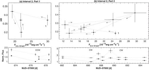
Spectral hysteresis in different epochs, along with the normalized soft 0.3–2 keV (grey points) and hard 2–10 keV (black points) fluxes plotted versus time (extract). The light curves for hard fluxes are shifted arbitrarily for a better resolution. In each plane, the start point is denoted by ‘1’. Grey arrows show the direction of increasing time.
The source showed a positive correlation between the X-ray and optical–UV fluxes (see Figs 12b and c and Table 10), hinting at the origin of 0.3–10 keV and UVOT-band photons by the same electron population and, predominantly, by the same synchrotron mechanism. The data points, making outliers from the scatter plot, could be related to a time shift between the X-ray and UVOT-band emissions, found by Kushwaha et al. (2018a) via the z-transformed discrete correlation function (Alexander 2013): the interval MJD 57640 − 57738 (the second half of intervals 5 and 6; see Figs 3e and f) showed a possible lag in the X-ray variability, while the X-rays lead the optical/UV by about 5–6 d during MJD 5785−57920 with the X-ray fluxes being anticorrelated with respect to the optical/UV. In Section 3.2, we reported some occasions when the optical–UV flux was declining along with enhanced X-ray activity. Such MWL behaviour of the source can be explained through a hardening in the electron energy distribution, shifting the entire synchrotron bump to higher energies and yielding a brightness decline at lower frequencies, while the X-ray brightness is rising (see Aleksic et al. 2015; Kapanadze et al. 2017). Note that the shift of the peak of the electron energy distribution with the increasing X-ray brightness is in accord with the simulations of Katarzynski et al. (2006) in the framework of the stochastic acceleration of electrons with narrow initial energy distribution, having the average energy significantly higher than the equilibrium energy.
Fig. 12(e) also demonstrates a positive correlation between the X-ray and IR J-band fluxes (see Table 10), although it is weaker than those between the XRT and UVOT-band fluxes. The weakness can be explained by the relatively sparsely sampled contemporaneous (|$F_{\rm 0.3-10 \, keV}$|, FJ) data set, as well as by the delay in the variability and the contribution of IR photons produced in the dusty torus. The evidence of the latter was reported by Agudo et al.(2011).
Although Fig. 12(f) shows a positive trend in the scatter plot |$F_{\rm 0.3-10 \, keV}$|– F15GHz, the correlation is below the 99 per cent confidence level. However, the absence of a significant correlation between the XRT- and OVRO-band emissions can be also explained by the delay in the radio-band flares and contribution from those jet regions which did not produce X-ray photons. Kushwaha et al. (2018b) also reported an absence of the correlation between the radio-band emission and those produced in other spectral ranges during 2015 December–2016 May.
Fig. 12(g) demonstrates an absence of a correlation between the weekly binned 0.3–10 keV and 0.1–300 GeV emissions. As discussed in Section 3.2, the source often was not detectable with 3σ significance in the LAT band during the here-presented period (more frequently than in previous years) and showed one of the lowest HE states during 2008–2017. It underwent increasing γ-ray activity along with an optical–X-ray flares only in interval 4 (see Fig. 3d). According to Kushwaha et al. (2018a), the LAT-band SED in the period MJD 57600 − 57750 was similar to the previous quiescent state SED, while it became harder in MJD 57750 − 57900, coincident with the detections at VHEs by VERITAS (with an extrapolated VHE SED smoothly matching the LAT data). These authors interpreted the LAT-band emission to be of EC origin with the seed low-energy photons produced in the broad-line region (BLR; the characteristic features of BLR was reported by Kushwaha et al. 2018b), yielding a lower variability compared to the optical–X-ray emission and the absence of the correlation with the latter in the here-presented period.
The optical–UV fluxes from the UVOT observations showed strong or very strong cross-correlations (see Figs 12h–i and Table 10), indicating their origin from the same electron population and emission mechanism. The optical (B−V versus B, B−U versus B, and V−U versus U) colour–magnitude diagrams do not show a bluer-when-brighter chromatism (see Figs 14a–c), similar to both the UVOT observations in 2005 May–2016 May (Siejkowski & Wierzcholska 2017) and those performed in the B and V bands with Automated Telescope of Optical Monitoring (ATOM) during the period 2007–2012 (Wierzcholska et al. 2015). Gupta et al. (2017) did not a detect a chromatism during the B-, V-, R-, and I-band observations during 2015 September–2016 May. However, the source exhibited this trend during the V- and B-band observations in 1973–1976 (Carini et al. 1992), as well as during the V- and R-band observations in 1993–1997 (Dai et al. 2011).
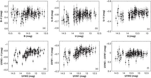
Colour–magnitude diagrams for the observations performed with UVOT.
Note that the source shows a weak bluer-when-brighter chromatism if we expand the study for the entire UVOT spectral range (e.g. UVW2−V index versus UVW2 magnitude, UVW1−V versus UVW1 etc.; see Figs 14(d)–(e) and Table 10 for the correlation coefficients), indicating a slight increase of the variability power from optical to higher frequencies (see also Table 5 for the values of the amplitude Fvar in each UVOT band during the interval discussed in Section 3.2). As for the separate UV energy range, no chromatism is evident here, similar to the optical frequencies (seeFig. 14f).
Similar to the X-ray emission, the optical–UV fluxes did not show a significant correlation with the 15 GHz and 0.1–300 GeV ones (see Figs 12j and k, respectively), and the latter were not correlated with each other (Fig. 12l). These results also confirm that the optical–X-ray, radio and γ-ray emissions were are not generated by the same electron population and emission mechanism.
6 SUMMARY
In this paper, we present the results of a detailed X-ray timing and spectral analysis of OJ 287 focused on the period of its significantly enhanced X-ray flaring activity during 2016 October–2017 April. The main results can be summarized as follows:
In this epoch, the 0.3–10 kV count rate from the XRT observations showed an increase by a factor of ∼10 compared to the quiescent level in 2016 April–May period, and OJ 287 became the sixth LBL/IBL source with the rate higher than 1 counts s−1. The mean count rate during 2016 October–2017 April |$\overline{\text{CR}}$| = 0.93, while this quantity was a factor of 4.5 smaller during the previous 300 XRT observations. The source underwent strong X-ray flaring activity on weekly time-scales and reached the highest historical 0.3–10 keV brightness (corresponding to 1.89 ± 0.03 counts s−1) in 2017 February. Along with these flares, the source showed 32 instances of 0.3–10 keV IDVs with fractional variability amplitudes of 7–60 per cent and the majority detected within the exposures shorter than 1 ks. In the framework of the SMBH model of OJ 287, a stronger X-ray flaring activity in 2016 October–2017 April could be related to the propagation of a stronger relativistic shock through the jet than those caused by the first impact triggering an optical–UV outburst, or those related to the previous BH encounters which led to the outbursts in 1994–1996 and 2005–2006.
Most spectra from the XRT observations of OJ 287 fitted well with a simple power-law model, yielding a wide range of the 0.3–10 keV photon index Γ = 1.90–2.90. In contrast to previous years, the source did not show very hard power-law spectra (Γ < 1.7) expected when the X-ray photons are produced only via the IC upscatter of low-energy synchrotron photons. However, we have found 29 spectra from this period showing an upward curvature due to the significant contribution made by X-ray photons of IC origin. While the spectral variability of OJ 287 showed a ‘harder-when-brighter’ spectral trend in previous years, the opposite trend was observed during this strong flaring activity which is explained by the emergence of a new soft component during X-rayflares.
Similar to X-rays, the source showed a strong outburst by factors of 4.6–6.5 in the UVOT bands V–UVW2 in 2016 October and kept its high optical–UV states during the next months, although the subsequent flares were not as strong as in the 0.3–10 keV energy range. A similar behaviour was observed also in the optical R and IR J bands, although the flares were characterized by lower amplitudes than those at the higher frequencies.
The X-ray flux showed a positive correlation with the optical–UV emissions, indicating its origin to be related to the same electron population, predominantly via the synchrotron mechanism. In contrast to the IR–X-ray emission, the source showed a considerably lower activity in the 0.1–300 GeV energy range, possibly related to its generation by different emission mechanism and electron population.
SUPPORTING INFORMATION
Supplementary data are available at MNRAS online.
Table 1.The XRT observations of OJ 287 in 2016 April–2017 June (extract).
Table 2. The results of the UVOT observations (extract).
Table 8. The results of the XRT spectral analysis with a simple power-law model (extract).
Figure 13. Spectral hysteresis in different epochs, along with the normalized soft 0.3–2 keV (grey points) and hard 2–10 keV (black points) fluxes plotted versus time (extract).
Please note: Oxford University Press is not responsible for the content or functionality of any supporting materials supplied by the authors. Any queries (other than missing material) should be directed to the corresponding author for the article.
ACKNOWLEDGEMENTS
BK, SK, and LT thank Shota Rustaveli National Science Foundation and Ilia State University for the grant FR/377/6-290/14. PR acknowledges the contract ASI-INAF I/004/11/0. This research has made use of the xrtdas software, developed under the responsibility of the ASDC, Italy, and the data from the OVRO 40-m monitoring program, which is supported in part by the NASA grants NNX08AW31G and NNX11A043G, and National Space Federation grants AST-0808050 and AST-1109911. This research has made use of data from the MOJAVE database that is maintained by the MOJAVE team (Lister et al. 2009) and the MAXI data provided by RIKEN, JAXA, and the MAXI team, as well as the data obtained through the High Energy Astrophysics Science Archive Research Center Online Service, provided by the NASA/Goddard Space Flight Center. This research has made use of data from the MOJAVE data base that is maintained by the MOJAVE team (Lister et al. 2009). This paper has made use of up-to-date SMARTS optical/near-IR light curves that are available at www.astro.yale.edu/smarts/glast/home.php. The UMRAO campaign was funded by the NSF grant AST 0607523 and by the NASA Fermi GI grants (cycles 2–6): NNX09AU16G, NNX10AP16G, NNX11AO13G, and NNX13AP18G. We thank the anonymous referee for his/her useful suggestions which helped to improve the quality of the paper.
Footnotes
See https://swift.gsfc.nasa.gov/analysis/xrt_swguide_v1_2.pdf for the XRT data reduction guide.
Since OJ 287 showed count rates much lower than ∼100 counts s−1, no pile-up correction was necessary for the observations performed in the WT regime; see Romano et al. (2006).
The threshold, adopted for a flux variability study using the MAXI data (Mihara, private communication).
See http://james.as.arizona.edu/ psmith/Fermi/
See also http://xte.mit.edu/ASM_lc.html for the 1.5–12 keV light curve obtained with the All-Sky Monitor onboard Rossi X-Ray Timing Explorer for X-ray behaviour of OJ 287 during 2005–2006.
See users.utu.fi/kani/1m/OJ_287_jy.html
For interval 1, we selected a longer time range than that covered by Swift observations of OJ 287 to include its HE and radio flares.
The difference between the Fvar in the 0.3–2 and 2–10 keV bands did not exceed the corresponding error range in interval 2.
