


ABSTRACT
Observational study of galactic magnetic fields is hampered by the fact that the observables only probe various projections of the magnetic fields. Comparison with numerical simulations is helpful to understand the real structures, and observational visualization of numerical data is an important task. In this paper, we investigate 8 GHz radio synchrotron emission from spiral galaxies, using the data of global three-dimensional magnetohydrodynamic simulations. We assume a frequency independent depolarization in our observational visualization. We find that the appearance of the global magnetic field depends on the viewing angle: a face-on view seemingly has hybrid magnetic field types combining axisymmetric modes with higher order modes; at a viewing angle of ∼70°, the galaxy seems to contain a ring-like magnetic field structure; while in edge-on view, only field structure parallel to the disc can be seen. The magnetic vector seen at 8 GHz traces the global magnetic field inside the disc. These results indicate that the topology of global magnetic field obtained from the relation between azimuthal angle and Faraday depth strongly depends on the viewing angle of the galaxy. As one of the examples, we compare our results at a viewing angle of 25° with the results of IC342. The relation between azimuthal angle and Faraday depth of the numerical result shows a tendency similar to IC342, such as the peak values of the Faraday depth.
1 INTRODUCTION
The origin and evolution of magnetic fields in spiral galaxies is a longstanding question. Radio observations of synchrotron radiation and Faraday rotation have provided various pieces of information of magnetic fields perpendicular to and parallel to the line of sight (LOS), respectively. The global magnetic field of spiral galaxies has been classified into axisymmetric spiral (ASS) seen in M31 or bi-symmetric spiral (BSS) in M81, based on the topology. Since the discovery of hybrid (ASS and BSS) structure in M51, many galaxies are classified into hybrid-types which consist of ASS and higher modes (Fletcher et al. 2011; Beck 2016). Such global magnetic fields are also known to co-exist with turbulent magnetic fields with comparable magnetic energy densities, which correspond to field strengths of micro gauss. (e.g. Beck 2007).
Such galactic magnetic fields are produced for billions of years by the maintenance mechanisms, which are related to the field topology. Parker (1970) and Parker (1971) proposed a galactic dynamo known as the alpha–omega dynamo and a mean-field galactic dynamo. That mechanism is able to produce toroidal magnetic fields from poloidal fields by the α-effect and poloidal fields from toroidal fields by the Ω-effect. It can amplify weak seed field into micro gauss field over 108 yr converting kinetic energy of thedifferentially rotating disc and energy from associated turbulent gas motions into magnetic energy. Extended dynamo theories were proposed in the 1980s. These models explain both ASS and BSS features of magnetic fields (Chiba & Tosa 1989; Fujimoto &Sawa 1987).
More recently, the importance of the magneto-rotational instability (MRI) was recognized (Balbus & Hawley 1991). Its effect on gaseous motions is taken into account in several global simulations of a galactic gas disc (Nishikori, Machida & Matsumoto 2006; Hanasz, Wóltański & Kowalik 2009; Machida et al. 2009, 2013). For instance, Machida et al. (2013) performed a three-dimensional (3D) magnetohydrodynamic (MHD) simulation of the galactic gas disc. They demonstrated the evolution of the galactic disc induced by the dynamo effect according to the MRI and Parker instabilities. Gressel, Elstner & Ziegler (2013) carried out hybrid dynamo simulations in which they considered the effects of both the MRI and the α–Ω dynamo excited by supernova explosions. Recently, the formation and evolution of a Milky Way-like disc galaxy is researched in full cosmological context with magnetic fields (Pakmor, Marinacci & Springel 2014).
In order to examine the topology of magnetic fields and understand their origin and evolution, theoretical predictions of observables are important. For example, using data of 3D MHD turbulence simulations, high-precision modeling, and observational visualization of diffuse ionized gas toward high Galactic latitudes was conducted (Akahori et al. 2013). Wide-field and high-spatial-resolution radio observations with future radio interferometers such as the Square Kilometre Array (SKA) would dramatically improve imaging quality in galaxy surveys, and would allow us to study complex structures that reflect the MRI-Parker instability. Moreover, future radio observations will achieve wideband polarimetry, which will deliver a new research dimension and will become a breakthrough of the study of galactic magnetic fields (e.g. Heald et al. 2015). For example, the use of Faraday tomography for astronomical objects has started (see e.g. Akahori et al. 2014; Ideguchi et al. 2014).
Radio broadband visualization is, however, challenging because the effect of depolarization is significant particularly at low frequencies (Burn 1966; Arshakian & Beck 2011). In this study, we attempt to perform broadband observational visualization of a spiral galaxy, using the data of a global 3D MHD simulation of a galactic gas disc (Machida et al. 2013). It aims to clarify the relation between projected observables and actual 3D structure of magnetic fields in our simulation. We introduce the numerical data in Section 2 and the method of calculation in Sections 3. The numerical results are shown in Section 4, followed by discussion and summary in Sections 5 and 6, respectively.
2 MHD SIMULATION OF A SPIRAL GALAXY
We analyze the results of global MHD simulations of a galactic gaseous disc. The simulation was performed in the cylindrical coordinate system (r, ϕ, |$z$|′). The simulation box size is defined in the radial direction as r < 56 kpc, in the azimuthal direction as |$0 \le \phi \le 2\pi$|, and in the vertical direction as −10 kpc < |$z$|′< 10 kpc, and is gridded evenly with cells of (250, 256, 640) in the (r, ϕ, |$z$|′) directions, respectively. In the main domain where we address in this paper, 0 kpc < r < 6 kpc and −2 kpc < |$z$|′ < 2kpc , the spatial resolution of the simulation is Δr = 50 pc and Δ|$z$|′ = 10 pc. With |$\Delta \phi=2\pi /256$|, the resolution of the azimuthal direction, rΔϕ, depends on r and is 25 pc at r = 1 kpc.
The initial condition of the simulation was an equilibrium torus threaded by weak azimuthal magnetic fields embedded in a non-rotating hot corona under the Miyamoto and Nagai potential (Miyamoto & Nagai 1975). The self-gravity of the gaseous disc, radiative cooling, and spiral-arm potential of the stellar disc were all ignored in their paper. The initial torus with the temperature |$10^4\, {\rm K}$| and the density |$1\, {\rm cm^{-3}}$| at |$r=10 \, {\rm kpc}$| changes its shape to the disc by redistribution of the angular momentum, because the magnetic turbulence caused by MRI transports the angular momentum outward. The resultant disc has the equatorial density of |$0.1 \, {\rm cm^{-3}}$| at |$r=2\sim 3 \, {\rm kpc}$|. Angular momentum of the gas in the disc is transported by the MRI, and the gas temperature increases to |$10^5 \, {\rm K}$| due to the adiabatic compression and the Joule heating by magnetic reconnection in the disc and the boundary layer between the disc and the halo. Magnetic field in the disc is amplified in such a high temperature plasma. The plasma β (the ratio of the gas pressure to the magnetic pressure) in the disc ranges from 5 to 100 and the averaged value becomes about 20. Note that the temperature varies with time but its fluctuation is small, because we did not consider gas cooling mechanism by radiation.
Although the disc magnetic field is tangled and becomes turbulent, structures of the global magnetic field in the disc and the halo have the compositions of the higher-order mode and ASS-like topologies, respectively. Such a duality seems to be consistent with the result of Faraday tomography for M51 (Fletcher et al. 2011).
Both the mean and turbulent components show similar peak strengths of about 10 μG. But the volume filling factor of such high strength regions is less than 0.1 in the disc and the volume-averaged strength in the disc is about a few μG. The average magnetic energy of the turbulent component is about three times larger than that of the mean (regular) component inside the gas disc, and they become comparable to each other in the halo region.
Our model exhibits a few magnetic spiral arms on the contour of the magnetic energy. But the magnetic spiral arms in the numerical results do not corresponds to the grand-design spiral such as M51, because we do not consider the cooling effect of the gas. The spiral galaxies showing grand-design spirals (e.g. M51 and so on) and higher star forming activities are beyond the scope of this paper. See Appendix A and Machida et al. (2013) for more details of the simulation data. Meanwhile, IC342 is one of the targets of our model (see recent review by Beck 2016). We attempt to compare IC342 with our simulation in Section 5.
3 OBSERVATIONAL VISUALIZATION
We consider observations of an external galaxy and calculate radio synchrotron observables such as the Stokes parameters and Faraday rotation measure. Since numerical simulation data has the physical values such as magnetic field vector and density at each grid point, we directly calculate the Faraday depth (FD), which is an integral of the LOS component of magnetic field weighted with the density. If the Faraday rotation occurs at the foreground of the synchrotron emitting source, the FD is equal to the Faraday rotation measure.
Fig. 1 shows the schematic drawing of the visualization region. The computational volume of the visualization is a cube (x, y, |$z$|) with sides of 20 kpc, which is centered on the galactic center. Two-dimensional maps are constructed with (Nx, Ny) = (200, 200) image pixels centered at the projected galactic center which corresponds to the bottom square in x–y plane on Fig. 1. Hence the image resolution becomes 100 pc. This resolution corresponds to |${\sim } 2\, \text{arcsec}$|, if we assume a galaxy is placed in the Virgo cluster at a distance of ∼20 Mpc.
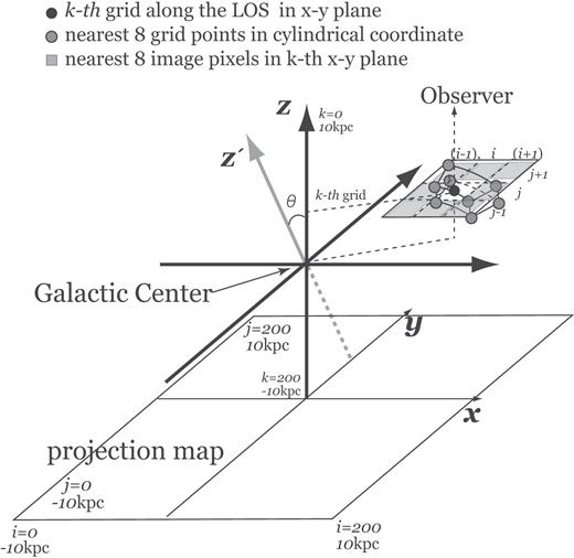
Schematic drawing of the visualization region. Black axises (x, y, |$z$|-axis) show the coordinate of the observational visualization. LOS components are along the |$z$|-axis. |$z^{^{\prime }}$|-axis shows the coordinate which is used in the MHD simulation of the galactic disc. A sectorial box denotes the computational grid box using MHD simulations which are adopted in the cylindrical coordinate system. Gray points are the grid points of the MHD simulation and black point is a grid point along the LOS (i, j, k). θ is an inclination angle of the galaxy. Gray hatched region show nearest eight cells of the image pixel (i, j) in k-th plane.
For each image pixel, we integrate observables along the |$z$|-axis. We incline the |$z$|′-axis of the cylindrical coordinate of the data along the y–|$z$| plane and the inclination angle, θ, is defined as the angle from the |$z$|-axis to the |$z$|′-axis; θ = 0° and θ = 90° correspond to face-on and edge-on view, respectively.
3.1 Procedure of visualization
According to Werner et al. (2015), electrons with energies greater than 100 GeV are confined to their source regions and trace the cosmic-ray source distribution closely. Because cosmic-ray electrons responsible for radio emission in 8 GHz in a magnetic field of 10 μG have energies of 7 GeV, the cosmic-ray electron is diffused from the magnetic spiral arm. The diffusion lengths of GeV electrons are about 1 kpc during their lifetime of a few 107 yr. Since this time scale is much more than the resolution in our model, the assumption of local equipartition is not valid. However, the diffusion of cosmic-ray is beyond the scope of this paper. If the total energy of cosmic-ray is comparable to the thermal energy and energy equipartition with magnetic fields is assumed, this contradicts β = 10 as derived in the MHD model (Appendix A). The energy spectral index p = 3 is adopted as a typical value (Sun et al. 2008).
4 RESULTS
We present the result of the simulation at a few tens of rotation periods at |$r =10\, {\rm kpc}$| as a representative case. It corresponds to about 48 billion years after the start of the simulation, at which both regular and turbulent magnetic fields are well-established by the MRI-Parker instability. Below, we show the results of face-on view, edge-on view, and intermediate inclination view in this order.
4.1 Face-on view
Fig. 2(a) shows the FD (FDave) map for the case of inclination angle 5°. It is clearly seen that the FD distribution is patchy and complex due to turbulent magnetic fields. Fig. 2(b) displays FDs in above-average bright regions of the simulated synchrotron total intensity (TI) at 8 GHz in order to highlight FDs at brighter regions.
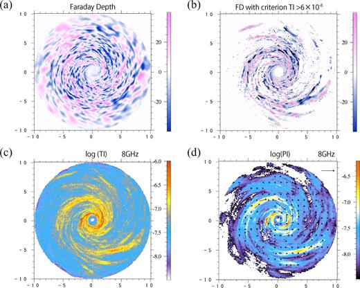
(a) FD contour map of the simulated spiral galaxy for an inclination angle θ = 5°. Both horizontal and vertical axes have units of kpc, and the FD has units of rad m−2. (b) Same as (a) but only the pixels with TI(8 GHz) larger than the average of TI(8 GHz) within the image are shown. (c) Simulated synchrotron TI at the observed frequency of 8 GHz. (d) Simulated PI at the observed frequency of 8 GHz, all in units of Jy/sr. Arrows indicate the magnetic vector (2χ + 90°) whose strength is normalized by the maximum strength in the map. The sample vector indicates the strength of magnetic field which is 20 per cent of the maximum one.
TI and polarized intensity (PI) at the observing frequency of 8 GHz are shown in Figs 2(c) and (d), respectively. Arrows show the magnetic vector, 2χ + 90°, with χ obtained from the Stokes Q and U (equation 9), whose strength is normalized by the strength of the maximum one in the map. The sample vector on Fig. 2(d) denote 20 per cent of the strongest magnetic strength. At some places, the direction of the magnetic field turns ∼180°across an arm/interarm. This is because the magnetic spiral arms have neutral currentsheets.
TI clearly shows spiral structure. Such patterns are also seen in PI, where PI and TI are similar to each other. Actually, Faraday rotation is weak at 8 GHz, and the magnetic vector, which is parallel to the spiral pattern of PI, traces the direction of magnetic fields. This indicates that TI and PI reflect the spiral magnetic-field structure inside the gas disc rather than magnetic fields in the halo.
4.2 Edge-on view
Fig. 3(a) shows the FD map for θ = 85°. The FD is mainly derived from the gas at the mid-plane of the LOS, because the azimuthal magnetic field is dominant and only the LOS component of magnetic fields can contribute to the FD. Similarly, FD around the rotation axis (x ∼ 0), at which denser gas exists, is rather small. Because the azimuthal magnetic field is dominant in the gaseous disc, the azimuthal magnetic field becomes parallel to the LOS around the |$z$|-axis.

Same as Fig. 2 but for θ = 85°.
There are reversals of the sign of FD along the radial direction. The reversals mean multiple inversions of the direction of the global azimuthal magnetic field. Actually, azimuthal magnetic fields, which emerged from the disc owing to the Parker instability, show periodic reversals. Such positive and negative FDs can be seen as stripes in the vicinity of the rotation axis. The length scale of emerging flux tubes from the disc to the halo are abouta few kpc, although the length depends on their radius. The striped FD patterns could be unique evidence that the magnetic flux flows out into the galactic halo successfully. Note that the pattern seems simply random around the rotation axis, if we focus on brighter regions (Fig. 3b). This means that it is difficult to identify the global patterns, if we only have low-sensitivity polarizationdata.
Figs 3(c) and (d) show the maps of TI and PI at 8 GHz, respectively. Overall, TI becomes larger towards the galactic mid-plane, because the global magnetic field is strongest in the disc. Structures seen in PI are similar to those seen in TI, and the magnetic vector nicely traces the global azimuthal magneticfield.
4.3 Intermediate inclination angles
Fig. 4 shows the results for the inclination angles θ = 25°, 45°, and 70° from left to right, respectively. As already mentioned in Fig. 3, the FD is relatively small along the rotation axis of the galaxy (x ∼ 0), since the dominant, azimuthal magnetic field is not parallel to the LOS and hence does not contribute to the FD. In contrast, PI, which intrinsically depends on the magnetic fields perpendicular to the LOS, is maximum around x ∼ 0 and weaker away from x ∼ 0.
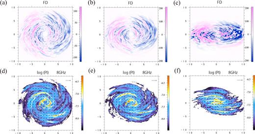
Maps of the simulated observables. Top and bottom panels show the FD and PI at 8 GHz. Also shown are the magnetic vector angles (2χ + 90°) as arrows. Panels from left to right show the results for the inclination angles θ = 25°, 45°, 70°, respectively. Both horizontal and vertical axes have units of kpc.
We find that the topology of the magnetic vector field in PI is different between small and large viewing angles, although we have used the same numerical data of a spiral galaxy. The magnetic vector field apparently can be explained with a mixed mode of ASS and higher modes with smaller scales for θ = 25°. As we increase θ, a ring-like structure partly mixes in the pattern inside2 kpc.
Fig. 5 shows an azimuthal variation of FD, which was calculated by integrating value of the FD in ranges of 3 kpc < r < 4 kpc and 4 kpc < r < 7 kpc, each of which are indicated with black and gray curves, respectively. To compare with the observation of IC342, the gray curves are integrated in the wide region. The dependence of the inclination angles is shown from top to bottom. The number of the reversals is comparable to the scale length of the Parker instability, which is about a few kpc in the azimuthal direction. The reversals which are shorter than 1 kpc are caused by the turbulent motion of the gas. The scale length is about 0.5 kpc in the vertical direction. This length corresponds to the vertical scale height. The number of the reversals in the range of 3 kpc < r < 4 kpc are larger than that in the range of 4 kpc < r < 7kpc. Because the width of the magnetic tube formed by the Parker instability is about 1 kpc, the resultants are cancelled by the integration. Remaining components of the reversal is driven by the Parker instability near the center region and mean components by the dynamo activities. In the almost face-on view (θ = 5°), these structures indicate that reversals of the vertical components along the LOS are observed. When the inclination angle becomes large, there are less reversals in the FD. Essentially, the higher mode with smaller scale is expected in our numerical simulation data because there are a few magnetic spiral arms. On the other hands, since the integrated region of the gray curves are larger than the scale length of the turbulence. The fluctuations in the curves are disappeared and ϕ-FD relations show a sinusoidal distribution (5b, c, d), which are typical structure of ASS. The FD curves of the outer region (gray one) still show the reversals of FD, which is considered to comborution of the ASS and the higher mode with smaller scale.
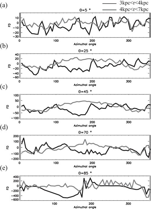
The azimuthal distribution of the FD. The black curves show the FD in the region of 3 kpc < r < 4 kpc, and gray curves show that in the region 4 kpc < r < 7 kpc. Top and bottom panels show the results of θ = 5° and 85°, respectively.
5 DISCUSSION
5.1 LOS distribution of magnetic fields
To link the projected observables to actual 3D structures, we plot the physical quantities along the LOS. Fig. 6 shows the cross sections toward the outer interarm(black) and the inner arm (gray) in the case of θ = 5°. As seen, the density distribution is smooth; the average number density is about 0.03 cm−3 in the disc and about 3 × 10⁻³ cm−3 in the halo. On the other hand, the LOS component of the magnetic field is disturbed and the local FDs within each computational cell indicate a complex distribution. The integration thus behaves like a random walk process; the integrated FD toward the arm is −18 rad m−2 although the maximum local positive FD along the LOS reaches about 4 rad m−2.
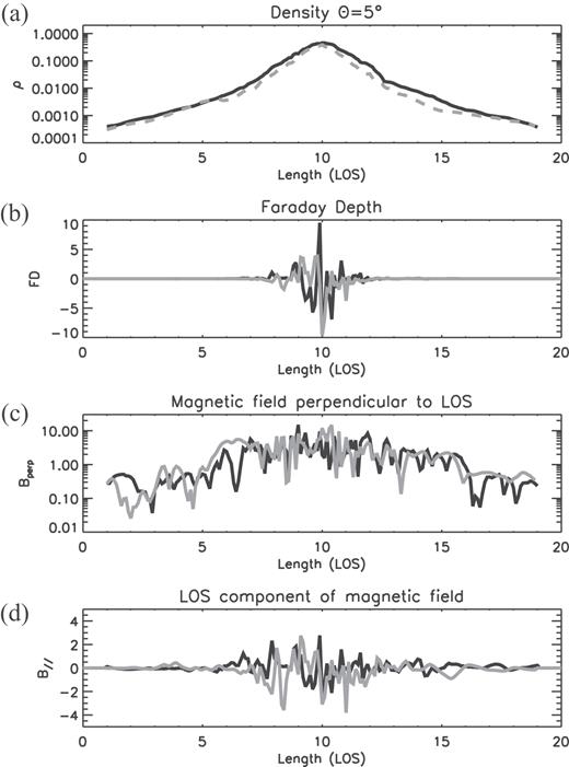
Distribution of physical quantities along the LOS (in kpc) for the inclination angle θ = 5°. Panels show (a) the gas number density in cm−3, (b) the local FD (in rad m−2) within each computational cell with a depth of 100 pc (c) |$B_{\bot }^2$| in (μG)2, and (d) B‖ in μG. Black and gray curves show the values toward the interarm (-3 kpc, 0 kpc) and the arm (2 kpc, -0.5 kpc), respectively. The galactic mid-plane is located at ∼10 kpc.
Note that B‖ has some peaks around LOS ∼8 kpc (∼2 kpc far from the equatorial plane). The peak magnetic fields are formed by the magnetic wind resulting from the flotation of the Parker instability. However, because the halo density is low, the FD induced by such magnetic fields does not significantly contribute to the total FD.
The same plots as Fig. 6 but toward the disc (black) and halo (gray) in the case of θ = 85° are shown in Fig. 7. The distribution of the local FD shows complex structure reflecting multiple reversals of B‖ due to the inversion of the azimuthal magnetic field in the radial direction. B‖ and B⊥ have comparable strengths of ∼10 μG, but FDs are very different and the FD in the halo is very small due to the low density in the halo.
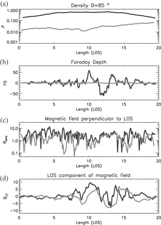
Same as Fig. 6 but for θ = 85°. Black and gray curves show the values toward the disc (3 kpc, 0 kpc) and the halo (−3 kpc, 3 kpc), respectively.
The resultant cumulative FD toward the disc is 151 rad m−2, although the local FDs show about |$-60 \, {\rm rad\, m^{-2}}$|.
5.2 Is X-field missing due to reduced outflows?
Our visualizations for the edge-on view do not indicate the X-shape structure of the magnetic vector, which is seen in, for example, NGC 253 (Heesen et al. 2009). Even though we choose a higher frequency such as 8 GHz, at which both Faraday rotation and depolarization are negligible and the magnetic vector thus traces the intrinsic direction of magnetic fields, the magnetic vectors indicate not vertical but azimuthal magnetic fields (e.g. Fig. 3b).
In our global MHD simulation of a spiral galaxy, it is possible that the growth of vertical magnetic fields is reduced on some level and thus the X-field does not exceed the azimuthal magnetic field. This is because the outflow velocity was |${\sim } 30\, {\rm km\, s^{-1}}$|, which is ∼10 per cent of that observed in starburst galaxies. A possible reason for such a low outflow velocity is that we ignored cosmic-ray pressure and/or we assumed high gas pressure initially. The effects of cosmic rays on magnetic instability were studied by several authors (e.g. Kuwabara, Nakamura & Ko. 2004; Khajenabi 2012; Suzuki, Takahashi & Kudoh 2014; Kuwabara & Ko 2015). According to these studies, the cosmic-ray pressure can support the growth of a magnetic instability such as the MRI or Parker instability, although the results depend on the diffusion of cosmic-rays and magnetic field structure. When starburst becomes dominant, the stellar wind could also produce powerful winds and cosmic-ray pressure could assist the acceleration of galactic winds.
5.3 Comparison with IC342
The FD reversal within the spiral arms are found in the galaxy IC342 which shows a low star formation rate and unclear spiral arms (Beck 2015). To compare to the observations, we made a plot of the FD in the spiral arms (see Fig. 2b). The periodical reversals of FD are observed in the spiral arms. Because the scale length correlates with the disc scale height, the reversal length of the FD signs are proportional to the radius. It means that these reversals are caused by the Parker instability. These results support to the observational results for IC342 and theoretical predictions of the Parker instability. Fig. 5(b) shows the relation between azimuthal angle and FD inside |$4 \, {\rm kpc} \lt r \lt 7 \, {\rm kpc}$| for θ = 25°, whose inclination angle seems to be IC342. The tendency of azimuthal angle – FD relation shows similar with IC342.
Since we ignored the cool components of galactic gas disc, the gas density and magnetic field strength will be underestimated. When we will consider the multitemperature distribution of galactic disc, these discrepancies will be resolved.
5.4 Enhancement of global magnetic fields
In our simulation, the volume-averaged energy of turbulent magnetic fields is three times larger than that of the mean magnetic field which is dominated by the azimuthal component in the disc. The peak strength of the mean azimuthal component, which corresponds to the magnetic spiral arm, is 70 per cent of that of the turbulent component. These magnetic spiral arms are much fainter than the grand-design spiral of the galaxies. This is because the temperature inside the disc becomes about 105 K, the turbulent cell becomes large. According to the Machida, Nakamura & Matsumoto (2006) which reported about the state transition of X-ray binaries, when the cooling effect worked in the accretion disc, the accretion disc shrinked in vertical direction with magnetic flux and mean magnetic fields enhanced inside the accretion disc. For the accretion disc case, the accretion disc became magnetically supported when the shrinking was stopped and the disc scale height of magnetically supported disc became 20 per cent of the gas pressure (high temperature) disc. The turbulent components of magnetic fields are dissipated inside the thin disc and the ordered field remained inside the disc. We speculate that magnetic field evolution through the gas heating and cooling qualitatively work in a similar manner between the galactic disc and the accretion disc. First, a part of neutral gas is ionized by supernovae, OB-star ultraviolet radiation and magnetic reconnection, etc. These ionization mechanisms are strongly couples with magnetic fields. Secondly, turbulence is generated and magnetic field is enhanced by the MRI and Parker instability in the radial direction. Thirdly, the ionized gas returns to neutral if the density is high enough to work the molecular cooling. The magnetic flux shrinks in vertical direction and the mean magnetic field enhances inside the disc. However, the scale height of warm H i components of galactic gas disc is comparable to the high temperature plasma, since there are extra energy inputs caused by the super novae and magnetic activities. Therefore, in the case of the galactic gaseous disc, we expect that the turbulent field is not much dissipated and the ordered magnetic energy will be comparable to the turbulent magnetic energy. In addition, the spiral potential of the galactic star disc has an important effect to produce the ordered magnetic fields.
6 SUMMARY
We summarize the points discussed in the present work:
PI becomes stronger towards the rotation axis of the galaxy, while FD shows the opposite tendency. This is because the azimuthal component of magnetic field is predominant inside the disc and thus the LOS component contributing to FD and the perpendicular component inducing PI depend on the distance from the rotation axis. These tendencies do not depend on the inclination angle of the galaxy.
TI and PI(8 GHz) are both stronger along denser magnetic spiral arms, where depolarization is insignificant at such high frequencies. The PA traces the orientation of the azimuthal magnetic field inside the disc.
An ASS-like structure appears in the magnetic-vector map for the case of θ = 85°, and one sine curve is seen in the azimuthal angle–FD relation. Meanwhile, since a few magnetic spiral arms are present in the numerical simulation data, a sine curve with three to four periods is expected in the azimuthal angle–FD relation in the case of θ = 5°. The topology, however, cannot be clearly classified as BSS with an inclination angle less than 70°. The ϕ–FD relations show a sinusoidal distribution which is typical structure of ASS.
An X-shape vertical structure is not observed in our results. It may be ascribed to the fact that our numerical results have weak outflows produced by Parker instability. If we include the effect of cosmic rays, the growth rate of the Parker instability becomes large and the outflow speed becomes high enough to explain the observations. Our assumption that the cosmic ray density is proportional to the magnetic energy should be improved in future works, so as to examine the structure in detail.
Although we ignored the spiral potential of a stellar disc, the spiral potential will be important in forming a magnetic spiral structure such as the BSS configuration. We plan to add this effect in the near feature. Suzuki et al. (2015) performed a 3D isothermal simulation of a galactic center region with axisymmetric gravitational potential, and they found that spatially dependent amplification of the magnetic field possibly explains the observed circular motion of gas in the galactic center region. Simulations of the distribution of cosmic rays are calculated by Werner et al. (2015). They showed that electrons with energies greater than 100 GeV are confined to their source regions and trace the cosmic-ray source distribution closely. And lower energy electrons diffuse to the interarm region.
Finally, we did not employ Faraday tomography, which is clearly complementary to our work and may be more powerful so as to deproject the LOS structure. It is, however, not trivial so far how we can translate the Faraday spectrum into real 3D structure of the galaxy (Ideguchi et al. 2014). We need further studies of both observational visualization and Faraday tomography for numerical data.
ACKNOWLEDGEMENTS
We are grateful to Dr. R. Matsumoto, Dr. K. Takahashi, and Dr. S. Ideguchi for useful discussion. We thank to Mr. Y. Morita who helped us a part of the visualization. We also thank to anomalous referee whose comments are very useful to improve our manuscript. Numerical computations were carried out on SX-9 and XC30 at the Center for Computational Astrophysics, CfCA of NAOJ (P.I. MM). A part of this research used computational resources of the HPCI system provided by (FX10 of Kyushu University) through the HPCI System Research Project (Project ID:hp140170).This work is financially supported in part by a Grant-in-Aid for Scientific Research (KAKENHI) from JSPS (P.I. MM:23740153, 16H03954, TA:15K17614, 15H03639).
REFERENCES
APPENDIX A: NUMERICAL SIMULATION OF GALACTIC GAS DISc
Machida et al. (2013) performed a 3D MHD simulation of the galactic gas disc. Below, we briefly summarize the evolution of magnetic field in the simulation.
The normalization of the velocity is |$v$|0 = (GM0/r0)0.5 where we assume the unit length is |$r_0=1 \, {\rm kpc}$| and |$M_0=10^{10}\, \mathrm{M}_{\odot }$|. The unit temperature is calculated by the unit velocity. This means that the unit velocity corresponds to the sound velocity. The thermal energy of the initial torus is balanced the gravitational energy which is made by the central black hole. They assumed the ratio of thermal energy to the gravitational energy is 0.05. Because the initial magnetic energy is defined by the plasma β which is the ratio of the gas pressure to magnetic pressure, magnetic energy is also proportional to the unit density of gas and has been defined by |$B_0=\sqrt{\rho _0 v_0^2}$|. In Machida et al. (2013), since the unit velocity and the unit density have been assumed about |$207\, {\rm km\, s^{-1}}$| and |$1\, {\rm cm^{-3}}$|, the unit strength of the magnetic fields is about |$26 \, {\rm \mu G}$|. Because the initial magnetic fields have been defined at |$10 \, {\rm kpc}$| and the ratio of thermal energy to gravitational energy at that radius have been assumed at 0.05, the initial fields strength have been about |$0.3 \, {\rm \mu G}$|.
Initial weak azimuthal magnetic fields are amplified initially by the differential rotation and by the MRI. After several rotation periods, averaged plasma β inside the disc becomes 10, which means that magnetic pressure is about 10 per cent of the gas pressure. Here, the rotation period at 1 kpc corresponds to the unit time of the simulation |$t_0=4.8 \times 10^6\, {\rm yr}$|.
When the disc reaches quasi-steady state, gaseous disc becomes turbulent and a strong magnetic flux forms locally, and he magnetic field strength reaches a few |$\mu \, {\rm G}$|. The volume filling factor for low–β (β ∼ 5) is 0.1. The density distribution of the gaseous disc near the galactic center shows a weak spiral structure and the magnetic fields also appear spiral, although we ignored the spiral potential produced by the stellar disc potential.
When the averaged magnetic pressure becomes about 10 per cent of the gas pressure in the disc, local magnetic pressure near the surface exceeds 20 per cent of the gas pressure and the Parker instability creates magnetic loops near the disc surface. Because the magnetic field strength parallel to the seed field grows faster than that of the opposite field, parallel fields satisfy the condition of the Parker instability earlier and buoyantly escape from the disc. The magnetic flux thus floats out from the disc because of the Parker instability.
Subsequently, since antiparallel to the seed fields remain inside the disc and are amplified by the MRI, mean azimuthal magnetic fields inside the disc reverse their direction. The reversed fields become a seed field for the next cycle. The direction of the azimuthal magnetic field in both radial and vertical directions inverts quasi-periodically. The time scale of the flotation cycle is about 10 times of a rotational period.
This mechanism has, however, not yet been proven by observations; it is still difficult to measure global magnetic fields in galaxies even with current large observational facilities such as the Jansky Very Large Array and Atacama Large Millimeter/Submillimeter Array.
The simulation adopted the initial weak azimuthal magnetic fields. Even if only an magnetic field is assumed at the beginning, numerical results show that multiple magnetic field arms are dominant in the disc owing to the development of magnetic turbulence. Meanwhile, in the halo region where an ASS magnetic field structure is dominant, magnetic lines of force are wound loosely.
We also have checked the dependence of the above results on azimuthal resolution, because the azimuthal resolution is sensitive to the saturation levels of MRI. The resultant ratio of the radial magnetic energy to the azimuthal magnetic energy were 0.12 and 0.13 with the azimuthal resolutions of 128 grids and 256 grids (the one that adopted in this paper), respectively. This value can be used to judge whether the most unstable wavelength of the MRI was resolved or not. From the comparison, we concluded that 128-grid model did not significantly differ from the results with 256-grid model in the nonlinear stage. The azimuthal spatial resolution adopted in our work is thus sufficient to reproduce the MRI.
