


ABSTRACT
Oxygen sequence Wolf-Rayet stars (WO) are thought to be the final evolution phase of some high-mass stars, as such they may be the progenitors of Type Ic SNe as well as potential progenitors of broad-lined Ic and long gamma-ray bursts. We present the first spectropolarimetric observations of the Galactic WO stars WR93b and WR102 obtained with FORS1 on the Very Large Telescope. We find no sign of a line effect, which could be expected if these stars were rapid rotators. We also place constraints on the amplitude of a potentially undetected line effect. This allows us to derive upper limits on the possible intrinsic continuum polarization and find Pcont < 0.077 per cent and Pcont < 0.057 per cent for WR93b and WR102, respectively. Furthermore, we derive upper limits on the rotation of our WO stars by considering our results in the context of the wind compression effect. We estimate that for an edge-on case the rotational velocity of WR93b is vrot < 324 km s−1 while for WR102 vrot < 234 km s−1. These correspond to values of vrot/vcrit < 19 per cent and <10 per cent, respectively, and values of log(j) < 18.0 cm2 s−1 for WR93b and <17.6 cm2 s−1 for WR102. The upper limits found on vrot/vcrit and log(j) for our WO stars are therefore similar to the estimates calculated for Galactic Wolf-Rayet (WR) stars that do show a line effect. Therefore, although the presence of a line effect in a single WR star is indicative of fast rotation, the absence of a line effect does not rule out significant rotation, even when considering the edge-on scenario.
1 INTRODUCTION
Wolf-Rayet (WR) stars are evolved massive stars characterized by the presence of broad emission lines in their spectra. They are the manifestation of dense winds (∼10−5 M⊙ yr−1) with velocities of several hundred to a few thousand km s−1 (Crowther 2007). WR stars are subdivided into three main types: nitrogen-rich (WN), carbon-rich (WC), and the rarer oxygen-rich (WO) stars. WO stars are very close to core helium exhaustion (e.g. Langer 2012) and are therefore the final evolutionary phase before these stars undergo core collapse, with a timescale of only a few thousand years (Tramper et al. 2015). This taxonomy also represents various degrees of stripping, with WN stars being hydrogen poor but retaining helium in their atmosphere, whereas both WC and WO are hydrogen and helium poor.
On the whole, WR stars are excellent candidates for the progenitors of stripped-envelope core collapse supernovae (CCSNe): The nitrogen-sequence (WN) stars are anticipated to end their lives as Type Ib (hydrogen poor / helium rich) SNe or IIb (transitional between Type II and Ib), whereas the carbon- and oxygen-sequence (WC and WO) WR stars are predicted to explode as Type Ic (hydrogen and helium poor) CCSNe (Filippenko 1997; Crowther 2007; Smartt 2009). Among the population of Type Ic SNe, a subset shows extremely broad spectral features caused by very high ejecta velocities (e.g. ∼30 000 km s−1 in SN 1997ef and SN 2014ad – Iwamoto et al. 2000; Stevance et al. 2017; Sahu et al. 2018) and are therefore labelled broad-lined Type Ic (Ic–bl) SNe.
Additionally, some Type Ic–bl SNe have been shown to accompany long gamma-ray burst counterparts (LGRB). SN 1998bw (Patat et al. 2001) was the first example of this association, while SN 2003dh (Stanek et al. 2003) is considered the archetype of cosmological GRB–SNe. Additionally, LGRB SNe have been showed to prefer lower metallicity environment (e.g. Modjaz et al. 2008). One of the more likely scenarios for the production of the LGRBs is the collapsar model (Woosley 1993), whereby a neutron star or black hole at the centre of the exploding star accretes matter via a disc that collimates a jet that ploughs through the envelope, thus driving the explosion. It has also been shown by Lazzati et al. (2012) that Type Ic–bl SNe without GRB counterpart could also be driven by similar central engines with shorter lifetimes, which result in choked jets producing no visible GRB but still imparting the energy required for the high velocities seen in the spectra of Type Ic–bl SNe. This explosion mechanism was suggested for Type Ic SN 2005bf and SN 2008D by Maund et al. (2007, 2009).
The production of such jets through core collapse requires the progenitor star to retain a high level of angular momentum (Woosley & Heger 2006), and WO stars have been proposed as candidate progenitors for LGRB–SNe (e.g. Hirschi, Meynet & Maeder 2005). Consequently, detecting rapid rotation in a helium-deficient WR star nearing the point of core collapse would offer observational support to such theoretical models (e.g. Yoon 2015). Rapid rotation in WR stars would cause wind compression effects such as described by Ignace, Cassinelli & Bjorkman (1996), resulting in aspherical winds. Additionally, electron scattering in WR winds is a polarizing process (Chandrasekhar 1960), and the direction of the polarization is tangential to the last surface of scattering. Since the star cannot be resolved, the observed polarization will be a sum of the components over the whole surface of the wind. An aspherical wind, such as that of rapidly rotating stars, will then result in incomplete cancellation of the polarization components, yielding a non-zero degree of continuum polarization. The presence of continuum polarization in WR stars manifests itself as a peak or trough in the degree of polarisation across strong emission lines (called line effect – e.g. Harries, Hillier & Howarth 1998), which is the result of a dilution of continuum polarization by unpolarized lineflux.
Evidence for such an effect has previously been reported in Galactic, Small Magellanic Cloud (SMC), and Large Magellanic Cloud (LMC) WN and WC stars, with amplitudes ranging from ∼0.3 to ∼1 per cent, and with an incidence of ∼20 per cent in the Milky Way and ∼10 per cent in the LMC (Harries et al. 1998; Vink 2007; Vink & Harries 2017). The study of Vink & Harries (2017) included spectropolarimetric observations for a binary WO star in the SMC but detected no line effect in this object. Because WO stars are only a few thousand years away from core collapse (Tramper et al. 2015), it is crucial to determine their rotational properties in order to constrain explosion models of Type Ic–bl and GRB–SNe.
In this work, we investigate the WR93b (WO3, Drew et al. 2004) and WR102 (W02, Tramper et al. 2015), whose time of explosion is estimated to be ∼9000 and 1500 yr, respectively (Tramper et al. 2015). They were selected on the basis that they are single Galactic WO stars accessible from the Very Large Telescope (VLT) in Chile . The observation and data reduction processes used are described in the the following section; in Section 3, we present the polarization obtained for our targets and infer upper limits on their intrinsic continuum polarization. Our results and analysis and their implications for the rotation velocity and fate of WR93b and WR102 are then discussed in Section 4; finally, our work is summarized in Section 5.
2 OBSERVATIONS AND DATA REDUCTION
Spectropolarimetric observations of WR93b and WR102 (see Table 1) were conducted under the ESO programme ID 079.D-0094(A) (P.I: P. Crowther). The data were collected on 2007 May 02 with the VLT of the European Southern Observatory (ESO) using the Focal Reducer and low-dispersion Spectrograph (FORS1) in the dual-beam spectropolarimeter ‘PMOS’ mode (Appenzeller & et al. 1998). The 300V grism was used in combination with a 1 arcsec slit, providing a spectral range 2748–9336 Å, and a resolution of 12 Å (as measured from the CuAr arc lamp calibration). No order sorting filter was used. Additionally, the observations were taken under median seeing conditions of FWHM = 0.7 arcsec. Linear spectropolarimetric data of our targets were obtained at four half-wave retarder plate angles: 0°, 22.5°, 45°, and 67°. Spectral extraction, following the prescription of Maund et al. (2007), was performed in iraf using routines of the fuss1 package as described by Stevance et al. (2017). The Stokes parameters were then calculated, and the data were corrected for chromatic dependence of the zero angles and polarization bias using fuss. To improve the signal to noise ratio the data were binned to 15 Å that, given the breadth of the emission lines (FWHM ∼200 Å), would not prevent us from resolving any potential line effect. Intensity spectra of WR93b and WR102 were retrieved by adding the flux spectra of each ordinary and extra-ordinary ray. Since we did not observe a spectrophotometric standard, however, we could not calibrate the flux spectra and simply show Stokes I (in counts). We note that Stokes I for both our targets is presented unbinned. Calibrated, de-reddened X-shooter spectra of WR93b and WR102 ranging from 3000 to 25000 Å can be found in Tramper et al. (2015).
3 POLARIZATION OF WR93B AND WR102
3.1 Observational properties
The reduced spectropolarimetric data of WR93b and WR102 are presented in Fig. 1. Before commenting on the characteristics of the polarization of our targets, we highlight specific spectral regions with noisy or spurious features: In WR93b, the degree of polarization (p) and polarization angle (θ) show greater levels of noise in the blue parts of the spectrum, particularly below 4400 Å; in the data of WR102, a broad peak in the degree of polarization (∼1 per cent deviation) and polarization angle (∼8° deviation) is seen between 7100 and 7600 Å. The latter feature cannot be a line effect as it is located in a region of the spectrum that is devoid of strong lines, and although its origin remains unknown (the details of our investigations are given in Section 3.2), we are confident it is of spurious nature. Given these considerations, the analysis presented in the rest of this study was performed without the spectral region below 4400 Å in WR93b, and the range 7100–7600 Å in WR102.
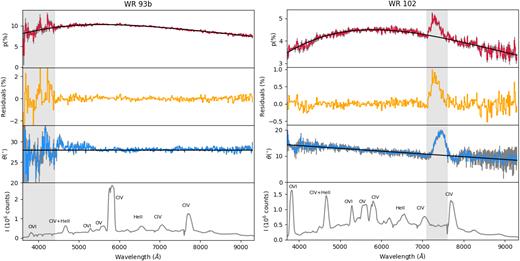
Spectropolarimetric data of WR93b (left) and WR102 (right). The panels, from top to bottom, respectively, the degree of polarization (red) and best Serkowski law fit (black); the residuals after Serkowski fit removal (orange); the polarization angle (blue); Stokes I (grey) and line identification. The grey areas represent the discrepant regions of the spectrum described in Section 3.1.
Excluding these wavelength ranges, the polarization in the direction of WR93b and WR102 rises up to ∼4.5 per cent and ∼10 per cent, respectively. Their polarization angles have distinct behaviours: WR93b exhibits a constant polarization angle of θ = 28.2°, whereas the polarization angle of WR102 shows a downward trend that can be fit with a line of the form θ = −1.08 × 10⁻³λ + 18.4 deg. A non-zero Δθ/Δλ can be explained either by the superposition of intrinsic and interstellar polarization (Coyne 1974) or by the presence in the line of sight of dust clouds with different particle sizes and alignments (Coyne & Gehrels 1966). The merit of these interpretations is discussed in Section 3.5.
3.2 7300 Å feature in WR102
In Section 3.1, we highlighted a prominent feature in WR102 spanning the wavelength range 7100–7600 Å. This peak was labelled as spurious and disregarded in our analysis. Here, we detail the steps taken in investigating the nature of this feature.
First, we explored whether the spike in polarization is intrinsic to the data. The fact that the feature is not associated with any strong line (as would be expected for a line effect present in the WR star) is, however, inconsistent with this idea. Additionally, plotting the polarization, calculated for each of the 12 sets of observations at four half-wave retarder plate angles (see Fig. 2), reveals that the shape and orientation (peak or trough) are highly variable from set to set, and no one set is consistent with another. To formally check whether the data are spurious, we look at the difference in instrumental polarization corrections (Δε, see Maund 2008) in this region of the spectrum. This property is expected to be 0 for polarization signals ≤20 per cent, and deviations indicate that the polarization does not reflect a real signal (Maund 2008). In Fig. 2, it is clearly visible that Δε is consistent with 0 across the spectrum but deviates significantly in the wavelength range that coincides with the discrepancy.
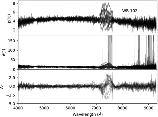
Superposed plots of the degree of polarization (p), polarization angle (θ), and instrumental signature correction difference (Δε) as calculated for each of the 12 sets of four half-wave retarder plate angles of WR102.
As the possibility that this feature was intrinsic to WR102 was ruled out, further investigation was required to understand its nature. We explored the possibility of a detector artefact by visually examining the 2D images, but none were found. Additionally, the data reduction of the polarization standard BD−12°5133 (observed immediately after WR102) showed no inconsistencies from the expected signal, and none of the WR93b data sets (observed before WR102) exhibited features such as that seen in WR102.
Finally, we tried different approaches to the calculation of the Stokes parameters from the ordinary and extra-ordinary fluxes:
Calculating q and u for each set of four half-wave retarder plate angles and computing the average.2
Averaging the normalized flux differences for each half-wave retarder plate angle and calculating q and u.
Averaging the ordinary and extraordinary rays for each half-wave retarder plate angle to then calculate the normalized flux differences and Stokes parameters.
As expected all these methods yielded consistent results including a visible discrepant feature around 7100−7600 Å.
Ultimately, we were not able to explain the origin of this feature as it does not seem to be either intrinsic to WR102 nor to be an issue with FORS1. However, since the rest of the data were unaffected, we carried out our analysis disregarding the affected region of the spectrum.
3.3 Interstellar polarization and limits on the line effect
The dust present in our Milky Way has a tendency to align along the magnetic field of the Galaxy that causes the light that passes through these dusty regions to become polarized. Both WR93b and WR102 are close to the Galactic plane and are obscured by a large amount of dust, as is evidenced by the high-reddening values reported by Tramper et al. (2015): E(B − V) = 1.26 and E(B − V) = 1.94 mag for WR93b and WR102, respectively. This results in high levels of Interstellar polarisation (ISP).
In order to retrieve the signal intrinsic to our targets, it would be ideal to quantify this ISP and remove it. To tackle this problem, one approach is to look at nearby standard stars that are intrinsically unpolarized, as any polarization detected for these objects can then be attributed to ISP. Unfortunately, the closest standard polarization stars in the Heiles (2000) catalogue were located over a degree away from our targets, making them inadequate probes of the interstellar medium between us and WR93b and WR102.
In this context, a precise estimate on the ISP in the direction of our targets is not possible, however, for the task at hand an absolute measure is not actually necessary. Indeed, as we are looking for the presence of a line effect, such as that observed in Harries et al. (1998), all that is needed is to investigate whether the polarization associated with emission lines shows any deviation from the observed continuum, which could be a blend of ISP and intrinsic continuum polarization. We can fit this underlying signal and remove it to then investigate whether the residual data are consistent with noise or if a line effect can be detected.
We performed fits of the degree of polarization of WR93b and WR102 with pmax, λmax, and K as free parameters using a non-linear least-squares optimizer (SciPy - Jones et al. 2017). The best-fitting parameters are summarized in Table 2, and the corresponding fits are shown in Fig. 1. Should there be any intrinsic continuum polarization, the shape of p(λ) will remain unchanged since polarization arising from Thomson scattering (such as can be the case in WR winds) has no wavelength dependence. Consequently, a blend of ISP and intrinsic continuum polarization will still be described by equation (1), although the values of pmax would differ from the ISP-only case. These fits can be subtracted to the polarization data observed for WR93b and WR102 to yield the residuals seen in Fig. 1. No evidence of a line effect is visible in either WR93b or WR102.
VLT FORS1 Observations of WR93b and WR102.
| Object | Date | Exp. Time | Airmass |
|---|---|---|---|
| (ut) | (s) | (mean) | |
| WR93b | 2007 May 02 | 48 × 150 | 1.12 |
| WR102 | 2007 May 02 | 48 × 70 | 1.06 |
| BD -12°5133 | 2007 May 02 | 8 × 12 | 1.14 |
| Object | Date | Exp. Time | Airmass |
|---|---|---|---|
| (ut) | (s) | (mean) | |
| WR93b | 2007 May 02 | 48 × 150 | 1.12 |
| WR102 | 2007 May 02 | 48 × 70 | 1.06 |
| BD -12°5133 | 2007 May 02 | 8 × 12 | 1.14 |
Best-fitting parameters of the Serkowski law fits to WR93b and WR102.
| Object | pmax | λmax | K |
|---|---|---|---|
| (per cent) | (Å) | – | |
| WR93b | 10.31 ± 0.01 | 5577 ± 18 | 1.25 ± 0.02 |
| WR102 | 4.50 ± 0.01 | 5795 ± 15 | 1.30 ± 0.03 |
| Object | pmax | λmax | K |
|---|---|---|---|
| (per cent) | (Å) | – | |
| WR93b | 10.31 ± 0.01 | 5577 ± 18 | 1.25 ± 0.02 |
| WR102 | 4.50 ± 0.01 | 5795 ± 15 | 1.30 ± 0.03 |
In order to place limits on the maximum amplitude a line effect could have while still being undetected, we measure the standard deviation of the residual polarization in the wavelength ranges corresponding to strong line regions, see Table 3.
3.4 Upper limit on the continuum polarization
As already stated in Section 3.3, there is no indication of a line effect in the polarization data of WR93b and WR102, however, we can use the limits we placed on the amplitude of a potentially undetected line effect (see Table 3) and equation (2) to put constraints on the continuum polarization in our targets. Our measurements of Iℓ for the strong emission lines of WR93b and WR102 are given in Table 3. An upper limit on the continuum that could remain undetected for each of these lines can then be estimated by substituting into equation (2) the measured Iℓ and our standard deviation value (in the corresponding wavelength range) in place of ΔP. The resulting values of Pcont are given in Table 3 and represent the maximum level of polarization that could be left unseen for each individual line. These upper limits on Pcont vary greatly from line to line, which is not unexpected as our proxy for ΔP is the standard deviation measured for a residual signal that is dominated by noise.
1σ limits on the polarization that could remain undetected in the signal associated with the strong emission lines of WR93b and WR102. The intensity at peak relative to continuum Iℓ as well as the derived upper limit on the intrinsic continuum polarization are also given.
| Line | Wavelength Range | 1σ (per cent) | Iℓ | >Pcont (per cent) |
|---|---|---|---|---|
| WR93b | ||||
| C iv λ5808 | (5705−5920) | 0.066 | 6.20 | 0.077 |
| C iv λ7724 | (7640−7840) | 0.118 | 2.13 | 0.173 |
| WR102 | ||||
| C iv λ4659 + C iv λ4686 + He ii λ4686 | (4600−4775) | 0.05 | 2.74 | 0.068 |
| O vi λ5290 | (5225−5360) | 0.03 | 1.13 | 0.057 |
| O v λ5590 | (5510−5690) | 0.035 | 0.79 | 0.079 |
| C iv λ5808 | (5705−5930) | 0.05 | 1.15 | 0.093 |
| He ii λ6560 + C iv λ6560 | (6380−6670) | 0.06 | 0.69 | 0.147 |
| C iv λ7724 | (7640−7870) | 0.11 | 1.95 | 0.166 |
In order to select a final upper limit from the values calculated, we need to consider that, as previously mentioned, the continuum polarization is not expected to be wavelength dependent. This means that any amount of polarization that goes undetected in one strong line will also be present in every other line and potentially be detectable. As a result, the effective 1σ limits on our values of Pcont for WR93b and WR102 will be the lowest values obtained from equation (2) and reported in Table 3, which do not necessarily involve the strongest emission line. Consequently, our upper limit on the continuum polarization Pcont of WR93b and WR102 are 0.077 per cent and 0.057 per cent, respectively.
3.5 ISP and Serkowski fits
It is now clear that the continuum polarization of WR102 and WR93b, should there be any, is low (<0.077 and <0.057 per cent, respectively). This implies that the polarization signal detected is overwhelmingly dominated by ISP, and our fitting parameters (summarized in Table 2) are representative of the ISP. Also, we can now deduce that the wavelength dependence of the polarization angle of WR102 mentioned in Section 3.1 is likely caused by two dust clouds overlapping in our line of sight with different particle sizes and grain orientation, rather than a superposition of ISP and continuum polarization.
In the case of both WR93b and WR102, we find λmax to be very close to the median value of 0.545 |$\mu$|m observed by Serkowski, Mathewson & Ford (1975) in the Milky Way. Regarding K, however, quantitatively comparing our estimates to the value assumed by Serkowski et al. (1975) is delicate since they provide no errors, and it is not clear which other values were tested and ruled out. On the whole, our values of K are close to the estimate of Serkowski et al. (1975), and they are not statistically inconsistent with each other. Performing a three parameter fit of the Serkowski law rather than assume K= 1.15 is an approach that has been employed by multiple studies (e.g. Martin, Clayton & Wolff 1999; Patat et al. 2015) and is motivated by the fact that the best value of K can be highly variable from target to target, even within the Milky Way (e.g. Martin et al. 1992).
Lastly, the Serkowski et al. (1975) study also reported the relation R ∼ 5.5 × λmax (|$\mu$|m), which we can use to estimate the total to selective extinction from our estimates of λmax. We find R = 3.1 and R = 3.2 for WR93b and WR102, respectively. These values are consistent with the estimates of Tramper et al. (2015) and standard interstellar medium values.
4 DISCUSSION
4.1 Rate of line effect in WR stars
In Section 3.3, we placed upper limits on the amplitude of the line effect that could go undetected in the polarization data of WR93b and WR102 (see Table 3). All of these limits have an amplitude significantly smaller than the amplitudes of the line effect observed in previous studies (<0.3 per cent, e.g. see Harries et al. 1998; Vink 2007), consequently it is safe to conclude that there is no line effect in either WR93b or WR102. Including the studies of Harries et al. (1998), Vink (2007), and Vink & Harries (2017), a sample of 82 WR stars has been observed with spectropolarimetry: 54 WN stars, 25 WC stars, and 3 WO stars. This sample includes Galactic, LMC, and SMC WR stars. Of these, 11 stars showed a line effect: nine WN stars, two WC star, and no WO stars. The incidence of the line effect on WR star populations in the Milky Way, SMC, and LMC is summarized in Table 4; the errors quoted on the percentages are the 68 percentile of the binomial confidence interval. Across all types, 13.4 ± 2.6 per cent of WR stars exhibit a line effect, however, when separated into sub-types we see that 16.6 ± 3.4 per cent of WNs showed a line effect, whereas only 8 ± 3.7 per cent of WCs and none of the WO stars did. It is important to note, however, that these values were obtained from data sets that are not uniform in quality and should therefore be considered with caution.
Incidence of WR stars found to have a line effect as a percentage of number of WR star observed. The errors are 68 percentile binomial confidence intervals. For each category, N indicates the total number of stars in the sample. References: 1: Coyne et al. (1988), 2: Whitney (1989), 3: Schulte-Ladbeck (1994), 4: Harries et al. (1998), 5: This work, 6: Vink (2007), 7: Vink & Harries (2017).
| Location | All types | WN | WC | WO | References | ||||
|---|---|---|---|---|---|---|---|---|---|
| (%) | N | (%) | N | (%) | N | (%) | N | ||
| Milky Way | 19.4 ± 4.8% | 31 | 23.8 ± 6.3% | 21 | 12.5 ± 8.0% | 8 | 0±−% | 2 | 1,2,3,4,5 |
| LMC | 10.3 ± 3.3% | 39 | 13.6 ± 5.0% | 22 | 5.9 ± 3.9% | 17 | – | 0 | 6, 7 |
| SMC | 8.3 ± 5.4% | 12 | 9.0 ± 5.9% | 11 | – | 0 | 0±−% | 1 | 7 |
| Total | 13.4 ± 2.6% | 82 | 16.6 ± 3.4% | 54 | 8 ± 3.7% | 25 | 0±−% | 3 | – |
On the whole, it seems clear that younger WR stars (i.e. nitrogen sequence) show a higher rate of line effect, although the apparent statistical significance is subject to the caveat mentioned above. This is in agreement with the study of Vink, Gräfener & Harries (2011), who pointed out the strong correlation between line-effect WR stars and the presence of ejecta nebulae. The latter are the aftermath of a recent strong mass-loss episode undergone by the stars during a red super giant or Luminous Blue Variable (LBV) phase and are therefore associated with WR sub-types in which hydrogen is present (i.e. late WN stars). This is consistent with the idea that heavy mass-loss also causes angular momentum loss, meaning that rapid rotation can be dissipated as a WR star further evolves.
4.2 Rotational velocities of WR93b and WR102
Stellar rotation, if rapid enough, can have dramatic effects on the surrounding winds. Bjorkman & Cassinelli (1993) demonstrated that for supersonic flow and a radial driving force, flow trajectories from an initially spherically symmetric wind lower the density at polar latitudes and increase the density at equatorial ones. This is known as the Wind-Compressed disc model. The main results were confirmed in hydrodynamical simulations by Owocki, Cranmer & Blondin (1994).
For smaller rotation speeds, Ignace et al. (1996) explored mild distortions from spherical flow, called wind compression zones (WCZ). We have employed this model to investigate how linear polarization depends on the stellar rotation speed. Details of the assumptions and approximations adopted for this model are summarized in Appendix A.
In order to place a limit on the rotation velocities of WR93b and WR102, we evaluated polarization using the WCZ approach for optically thin scattering. Although WR winds are optically thick to electron scattering, the rise of optical depth shows a sharp increase at the very inner wind owing to the rapid drop in wind velocity, with a corresponding fast increase of density. This is where multiple scattering can lead to depolarization, where the wind is mostly spherical, and where finite star depolarization effects are strongest (Cassinelli, Nordsieck & Murison 1987). We expect that most of the polarization is formed where the optically thin scattering limit applies.
The WCZ models result in a prediction of the net linear polarization as a function of wrot = vrot/v∞. Terminal wind speeds of 5000 km s−1 are reported for both WR93b and WR102 (Tramper et al. 2015) and were used to obtain the solid lines shown in Fig. 3. The errors on the relationship between degree of polarization and rotational velocity are dominated by the errors on v∞3 and are represented by the dashed lines in Fig. 3. It is worth reiterating that one underlying assumption of our model is a β = 1 velocity law. This is a good approximation for the inner wind (see fig. 8 in Gräfener & Hamann 2005), which is most relevant to the wind compression effect.
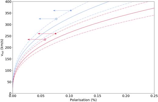
Relation between polarization and rotational velocity for WR93b (blue) and WR102 (red). The dashed lines represents 1σ limits. The polarization limits derived in Section 3.4 are marked by the open circles, while the polarization limits scaled by <sin i > 2 are represented by the star markers.
Note that the curve is for a model that assumes the axisymmetric wind is viewed edge-on. Such an inclination maximizes the observed polarization and minimizes the limit placed on the rotation speed. For optically thin electron scattering, the polarization scales as sin2i, where i is the viewing inclination angle. Consequently, for a given upper limit to the polarization, the limit placed on the rotation speed of the star is inverse to this factor. While it is statistically unlikely to observe either WR93b or WR102 as edge-on, it is also unlikely that either, and especially that both, would be observed near pole-on.
In addition to considering the calculated polarization limits (which represent the edge-on case), we scaled the polarization limits found in Section 3.4 for <sin 2i > = 0.75 to represent the expected value of a star with random inclination. The intersection of the polarization limits, and the upper limits on the curves of WR93b and WR102 are indicated by the markers on Fig. 3. The corresponding rotational velocities are summarized in Table 5.
Summary of the upper limits on the rotational velocities of WR93b and WR102 obtained for a 90° inclination and a random inclination as well as the resulting limit on vrot/vcrit and specific angular momentum j = vrotR*.
| WR | Scaled p | vrot | vrot/vcrit | log (j) |
|---|---|---|---|---|
| (%) | (km s−1) | (%) | (cm2 s−1) | |
| i = 90° | ||||
| 93b | <0.077 | <324 | <19 | <18.0 |
| 102 | <0.057 | <234 | <10 | <17.6 |
| <sin i > | ||||
| 93b | <0.190 | <457 | <26 | <18.1 |
| 102 | <0.141 | <327 | <14 | <17.7 |
| WR | Scaled p | vrot | vrot/vcrit | log (j) |
|---|---|---|---|---|
| (%) | (km s−1) | (%) | (cm2 s−1) | |
| i = 90° | ||||
| 93b | <0.077 | <324 | <19 | <18.0 |
| 102 | <0.057 | <234 | <10 | <17.6 |
| <sin i > | ||||
| 93b | <0.190 | <457 | <26 | <18.1 |
| 102 | <0.141 | <327 | <14 | <17.7 |
It should be noted that the wind compression effect considered here does not include the role of additional rotational effects such as gravity darkening or oblateness. For the case of fast-rotating B stars, Cranmer & Owocki (1995) found that the inclusion of these non-radial forces would weaken the wind compression effect, which would lead to rotational velocity underestimates of 5–10 per cent. Unfortunately, no similar study exists for WR stars and such an investigation is beyond the scope of this paper, however, considering the B star case our upper limits on rotational velocities may be even higher if other rotational effects were taken into account.
Lastly, we point out that our upper limits on the rotational velocity of WR102 are much lower than the rotational velocity of ∼1000 km s−1 inferred by Sander, Hamann & Todt (2012) from studying the shape of the emission lines in the spectrum. The model used by Sander et al. (2012) used a number of assumptions and physical stellar parameters that are not consistent with this study, which could explain the difference in values. Most notably they assumed spherical symmetry and used physical parameters significantly different from those adopted here. Additionally, assuming a rotational velocity of 1000 |$\mathrm{ km \,\, s^{-1}}\,$| for WR102 would result in |$v_{\rm rot}/v_{\text{crit}} = 44^{+10}_{-8}$| per cent (see Section 4.3), which is much greater than observed in Galactic WR stars that did show a line effect (Harries et al. 1998). These factors suggest that vrot = 1000 |$\mathrm{ km \,\, s^{-1}}\,$| may be an overestimate for WR102, warranting a re-evaluation of the Sander et al. (2012) approach using parameters based on Gaia DR2 distance.
4.3 vrot/vcrit and specific angular momentum j
The recent DR2 data release of Gaia parallaxes (Luri et al. 2018) allowed us to calculate new distances to WR93b and WR102: 2.3 ± 0.3 kpc and 2.6 ± 0.2 kpc, respectively (Rate et al. in preparation). We can use these estimates to calculate updated values of stellar parameters from the Tramper et al. (2015) values (see their table 4) that are summarized in Table 6. The corresponding values of vcrit are found to be: |$v_{\text{crit}}=1734^{+545}_{-415}$||$\mathrm{ km \,\, s^{-1}}\,$|and |$v_{\text{crit}}=2286^{+528}_{-429}$||$\mathrm{ km \,\, s^{-1}}\,$| for WR93b and WR102, respectively. The resulting limits on the values of vrot/vcrit for a 90° and a random inclination are also summarized in Table 5.
Summary of the physical parameters of WR93b and WR102 and their calculated critical velocities.
| WR | M⋆ | log(L⋆) | R⋆ | vcrit | d |
|---|---|---|---|---|---|
| M⊙ | L⊙ | R⊙ | km s−1 | kpc | |
| 93b | |$7.1^{+2.4}_{-1.8}$| | 4.96 ± 0.22 | |$0.39^{+0.11}_{-0.09}$| | |$1734^{+545}_{-415}$| | 2.3 ± 0.3 |
| 102 | |$7.0^{+1.8}_{-1.4}$| | 4.95 ± 0.17 | |$0.23^{+0.05}_{-0.04}$| | |$2286^{+528}_{-429}$| | 2.6 ± 0.2 |
Additionally, based on our upper limits of vrot for our WO stars, we can calculate upper limits for their specific angular momentum (j), which allows us to compare WR93b and WR102 to the threshold of the collapsar scenario (j ≥ 3 × 1016 cm2/s, MacFadyen & Woosley 1999) as well as other Galactic WR stars (Gräfener et al. 2012). The values of j calculated for both targets for an inclination of 90° and a random inclination are summarized in Table 5.
We find that both our limits on vrot/vcrit and j are very similar to the values calculated for Galactic WR stars showing a line effect (Harries et al. 1998; Gräfener et al. 2012). Note that the rotational velocities inferred for the WR stars in Harries et al. (1998) and Gräfener et al. (2012) were calculated using spectroscopic and photometric variability, which rely on fewer assumptions than the method employed here and are therefore more robust. We can see that the limits placed on j for our WO stars exceed the threshold for the collapsar model and therefore cannot exclude WR93b and WR102 being LGRB progenitors. However, LGRBs are seen to prefer low-metallicity environments (Graham & Fruchter 2013), making this scenario highly unlikely.
Finally, these results indicate that the absence of a line effect is not necessarily synonymous of insignificant rotation. When investigating the presence of rotation of WR stars using spectropolarimetry, caution is therefore required when interpreting non-detections as the absence of a line effect is not a direct measure of the absence of rapid rotation.
5 CONCLUSIONS
In this work, we presented FORS1 spectropolarimetric data of WR93b and WR102, which is the first spectropolarimetric data set obtained for Galactic WO stars. The main results of our work are as follows:
We find no line effect for either WR93b and WR102.
We deduced upper limits for continuum polarization of Pcont < 0.077 per cent and Pcont < 0.057 per cent for WR93b and WR102, respectively.
The corresponding upper limits on the rotational velocity for an edge-on case and a velocity law β = 1 are vrot < 324 |$\mathrm{ km \,\, s^{-1}}\,$| and vrot < 234 |$\mathrm{ km \,\, s^{-1}}\,$|, for WR93b and WR102, respectively.
We then found upper limits on vrot/vcrit: <19 per cent and <10 per cent for WR93b and WR102, respectively.
Lastly, we calculated upper bounds for the specific angular momentum of WR93b and WR102: log(j)<18.0 and log(j)<17.6 (cm2/s), respectively. These values do not exclude the collapsar model, and we therefore cannot constrain the fate of WR93b and WR102, although the preference of LGRBs for low-metallicity environment makes this outcome highly unlikely.
Our upper limits on vrot/vcrit and log(j) were found to be similar to values found for Galactic WR stars showing a prominent line effect. Consequently, this shows that the absence of a line effect is not necessarily synonymous of the absence of rapid rotation.
ACKNOWLEDGEMENTS
The authors would like to thank the staff of the Paranal Observatory for their kind support and for the acquisition of such high-quality data on the program 079.D-0094(A). We are grateful to Simon Goodwin and Liam Grimmett for their insight on statistics. H. F. Stevance is supported through a PhD scholarship granted by the University of Sheffield. R. Ignace acknowledges support by the National Science Foundation under Grant No. AST-1747658. The research of J. R. Maund is supported through a Royal Society University Research Fellowship. The following packages were used for the data reduction and analysis: matplotlib (Hunter 2007), astropy (The Astropy Collaboration 2018), numpy, scipy, and pandas (Jones et al. 2017).
Footnotes
Method normally used by fuss.
WO radii are relatively secure, despite Tramper et al. (2015) citing an uncertainty of ∼10 per cent in stellar temperatures. Higher (lower) temperatures will lead to smaller (larger) radii together with larger (smaller) bolometric corrections that, in turn, require higher (lower) luminosities and larger (smaller) radii for the adopted absolute visual magnitudes.
REFERENCES
,
APPENDIX A: RELATION BETWEEN ROTATION AND POLARIZATION
This appendix briefly reviews key ideas about Wind Compression theory (Bjorkman & Cassinelli 1993; Ignace et al. 1996), approximation formulae to characterize the density distribution of rotating stellar winds (Ignace 1996; Bjorkman, private comm.), and our use of these models in relating observed polarization to stellar rotation speeds.
A1 Approximations for Wind Compression effects
The Wind-Compressed disc model of Bjorkman & Cassinelli (1993) was developed to characterize the density and velocity distributions for the supersonic portion of a stellar wind, under the assumption of a radial wind driving force. In developing observational diagnostics, it is useful to have approximation formulae for the Wind Compression formalism to explore parameter space more rapidly. The following summarizes an approach appearing in Ignace (1996).
A2 Optically thin scattering polarization
The calculation of electron scattering polarization from an unresolved source involves a volume integral over the scattering region. Because the wind is axisymmetric, we employ the approach of Brown & McLean (1977), allowing for the finite star depolarization effect of Cassinelli et al. (1987), and accounting for stellar occultation. We loosely follow the expressions of Brown, Ignace & Cassinelli (2000) for the luminosity of polarized light, LQ. The Stokes-U component is zero for axisymmetry, with the observer axes defined by the stellar symmetry axis projected on to the sky.
Author notes
Royal Society Research Fellow
