


ABSTRACT
We study high-energy γ-rays observed from Cyg X-3 by the Fermi Large Area Telescope and the 15-GHz emission observed by the Ryle Telescope and the Arcminute Microkelvin Imager. We measure the γ-ray spectrum averaged over strong flares much more accurately than before and find it well modelled by Compton scattering of stellar radiation by relativistic electrons with the power-law index of ≃3.5 and a low-energy cutoff at the Lorentz factor of ∼103. We find a weaker spectrum in the soft spectral state but only upper limits in the hard and intermediate states. We measure strong orbital modulation during the flaring state, well modelled by anisotropic Compton scattering of blackbody photons from the donor by jet relativistic electrons. We discover a weaker orbital modulation of the 15-GHz radio emission, which is well modelled by free–free absorption by the stellar wind. We then study cross-correlations between radio, γ-ray, and X-ray emissions. We find the cross-correlation between the radio and γ-ray emission peaks at a lag less than 1 d, while we detect a distinct radio lag of ∼50 d with respect to the soft X-rays in the soft spectral state.
1 INTRODUCTION
Cyg X-3, one of the first discovered X-ray binaries (Giacconi et al. 1967), is a unique and puzzling system. The nature of its compact object remains uncertain; Zdziarski, Mikołajewska & Belczyński (2013) considered the radial velocity measurements of Hanson, Still & Fender (2000) and Vilhu et al. (2009) as well as constraints from the donor mass-loss rate and the orbital-period change and obtained the compact-object mass range of |$M_{\rm c}\simeq 2.4_{-1.1}^{+2.1} \,{\rm M}_{\odot }$|. Koljonen & Maccarone (2017) did not confirm the measurements of Hanson et al. (2000) in their infrared (IR) spectroscopic measurements and noted that it was possible that the velocity amplitude of Hanson et al. (2000) traced the motion of the stellar wind rather than of the star. Nevertheless, Koljonen & Maccarone (2017) found the most likely mass range of Mc ≲ 5 M|$\odot$|. Thus, the current constraints allow either a neutron star or a low-mass black hole (BH). The presence of a BH appears to be favoured by considering various aspects of the X-ray and radio emission (Hjalmarsdotter et al. 2008, 2009; Szostek & Zdziarski 2008; Szostek, Zdziarski & McCollough 2008; Koljonen et al. 2010, 2018). Also, Zdziarski, Misra & Gierliński (2010) have shown that the differences between the shapes of the X-ray spectra of Cyg X-3 in its hard spectral state and those of confirmed accreting BH binaries can be accounted for by Compton scattering in the strong stellar wind from the donor, which also would account for the lack of high frequencies in its power spectra (Axelsson, Larsson & Hjalmarsdotter 2009). On the other hand, Burke, Gilfanov & Sunyaev (2017) showed that weakly magnetized neutron-star X-ray binaries in the hard state have similar spectral properties to their BH counterparts but lower electron temperatures and softer spectra (which confirms some previous studies). This may be compatible with Cyg X-3 hosting a neutronstar.
Cyg X-3 is the only known binary in the Galaxy containing both a compact object and a Wolf-Rayet star (van Kerkwijk et al. 1992, 1996; van Kerkwijk 1993; Fender, Hanson & Pooley 1999). Given its very short period of P ≃ 0.2 d (unusual for a high-mass binary), it is a likely progenitor of a close double degenerate system, after the donor explodes as a supernova (Belczyński et al. 2013). The merger will then be associated with emission of gravitational waves, which has important implications for the detectability of similar extragalactic systems by LIGO and VIRGO (Belczyński et al. 2013).
The most recent distance estimate is the geometric one from dust-scattering haloes of D ≃ 7.4 ± 1.1 kpc (McCollough, Corrales & Dunham 2016), which agrees well with the estimate of |$7.2^{+0.3}_{-0.5}$| kpc of Ling, Zhang & Tang (2009) obtained with the same method. A similar distance range is also preferred based on considering constraints on the donor mass (Koljonen & Maccarone 2017). At this D, its absorption-corrected bolometric X-ray luminosity reaches several times 1038 erg s−1 in its brightest (soft) state, i.e. it reaches the Eddington limit for a 4M|$\odot$| BH and exceeds it for a neutron star (Zdziarski, Segreto & Pooley 2016b, hereafter ZSP16). Among X-ray binaries, Cyg X-3 is the brightest and most highly variable radio source (McCollough et al. 1999), also showing resolved jets (Mioduszewski et al. 2001; Miller-Jones et al. 2004; Tudose et al. 2007; Egron et al. 2017) on the size scale from a few up to several tens of mas (at 7 kpc, 25 mas corresponds to the projected distance of 1 light day). However, larger radio structures are also observed (Martí, Paredes & Peracaula 2001) on the scale of 1 arcsec (corresponding to 40 light days).
Its high-energy (HE) γ-ray emission has been discovered by the Fermi Large Area Telescope (LAT; Atwood et al. 2009) and AGILE (Tavani et al. 2009a) in the soft spectral state (Fermi-LAT Collaboration 2009, hereafter FLC09; Tavani et al. 2009b). The GeV power-law emission and its orbital modulation appear to be due to Compton up-scattering of the stellar emission from the companion WR star by relativistic electrons in the jet (Dubus, Cerutti & Henri 2010). Cyg X-3 is one of only two X-ray binaries that are certainly powered by accretion for which HE γ-ray emission has been detected at a high statistical significance; the other one being Cyg X-1 (also a high-mass X-ray binary, hereafter HMXB), where the γ-ray emission is, however, much weaker (Zanin et al. 2016; Zdziarski et al. 2017). Among low-mass X-ray binaries (LMXBs), a γ-ray flare from V404 Cyg was detected at an ∼4σ significance during the 2015 outburst (Loh et al. 2016a). The relatively strong radio and HE γ-ray emissions in Cyg X-3 may be due to interaction of the jet with the stellar wind, which is very dense near the compact object in this close Wolf-Rayet system, and subsequent formation of recollimation shocks (e.g. Yoon, Zdziarski & Heinz 2016 and references therein).
The presence of a powerful jet in soft states in Cyg X-3 is significantly different from the behaviour of accreting BH LMXBs, where a short-duration transient jet can appear during hard-to-soft transitions (Fender, Belloni & Gallo 2004), and the radio emission is strongly quenched in the soft state (Corbel et al. 2000). As shown by Koljonen et al. (2010), strong radio flares in Cyg X-3 occur during the transition from the softest (hypersoft) states to harder ones in the opposite direction and at much lower hardness ratios than those in LMXBs. On the other hand, accreting BH binaries in the hard state feature a steady compact jet, emitting partially self-absorbed synchrotron radio-mm-IR emission. This is then similar to Cyg X-3, which has a hard state with relatively strong radio emission correlated with soft X-rays, whose correlation is similar to that in BH binaries (Corbel et al. 2013; ZSP16). Therefore, we can expect some HE γ-ray emission of Cyg X-3 in its hard state, similar to the case of Cyg X-1.
In this work, we obtain HE γ-ray spectra in the flaring, hard, intermediate, and soft states. Furthermore, we present and study 15-GHz monitoring data from the Ryle Telescope and the Arcminute Microkelvin Imager (AMI). The latter data cover the entire duration of the LAT observations analysed here. We measure and model the orbital modulation of both radio and HE γ-ray emissions. We then study correlations between the γ-rays and radio and X-ray emissions.
2 DATA
2.1 FERMI LAT data reduction
We have analysed the available Fermi/LAT data (MJD 54682–57982) coming from the direction of Cyg X-3 using the latest version of the Fermi Science Tools (v10r0p5) with the P8R2_CLEAN_V6 instrument response functions. We have used the standard value of the zenith angle cut of zmax = 90°.
Similarly to FLC09, we have considered the presence of the nearby γ-ray pulsar PSR J2032+4127, located about 30′ away from Cyg X-3. That pulsar appears to be a member of a highly eccentric (e ∼ 0.95), long-period (∼25–50 yr), binary with a massive Be star (Lyne et al. 2015; Takata et al. 2017), and the orbital motion causes strong variations of the pulse period. The spin ephemeris is given by Lyne et al. (2015), and according to it, the pulse curve of PSR J2032+4127 is dominated by two strong peaks at phases 0.13–0.19 and 0.62–0.70. However, PSR J2032+4127 is now approaching the periastron, which resulted in strong departures of the ephemeris from that of Lyne et al. (2015) after 2015. Based on the LAT data, we have been unable to update the ephemeris. Therefore, we have been unable to use the approach of FLC09 of using only the off-pulse intervals. Instead, we have relied on taking into account the emission of the pulsar (along with other sources in the region) in our fitting of the LAT data (see below). We also note that the pulsar flux contribution at the position of Cyg X-3 is much lower than that of Cyg X-3 when it is in the flaring state, and also no GeV flux enhancement from PSR J2032+4127 was observed while approaching the periastron (Takata et al. 2017). Still, we have compared the results for the Cyg X-3 spectra in different states obtained using all the data and those subtracting the pulsar peaks according to Lyne et al. (2015) and found virtually no differences. Therefore, we have used the entire data in this work.
In order to take account of the broad Fermi/LAT point-spread function at energies studied by us (80 MeV–300 GeV), we consider a large, 25° × 25°, region of interest (ROI) around the Cyg X-3 position. We include in the modelling all sources within the ROI from the 4-yr Fermi catalogue (Fermi-LAT Collaboration 2015; 3FGL). We have used the standard templates for the Galactic (gll_iem_v06.fits) and extragalactic (iso_P8R2_CLEAN_V6_v06.txt) diffuse backgrounds. The catalogue sources were assumed to be described by the 3FGL spectral models with all parameters except the normalizations frozen to their catalogue values. In order to avoid possible systematic effects, we have also included into the model the 3FGL catalogue sources located up to 10° beyond the ROI with all parameters fixed to their catalogue values. For Cyg X-3, we adopt the power-law model with the slope 2.7 reported previously in FLC09. The spectral analysis has been performed with the python tools.1 The upper limits are calculated with the IntegralUpperLimits python module for detection significances of TS (test statistic; see Mattox et al. 1996) <4, which correspond to a 95 per cent (≃2σ) probability for the energy flux to be lower than the limit.
We then built the TS map in a 5° × 5° region around the position of Cyg X-3 in the 1–300 GeV energy band, see Fig. 1. We see a number of residuals along the Galactic plane, which we mark as n1–n6. Since almost all of them are at very low Galactic latitudes, where we expect the highest uncertainties, most of them seem to be diffuse residuals unaccounted for in the diffuse background model. The only residual that can be identified in any catalogue is n1, which was present in the first Fermi catalogue (Fermi-LAT Collaboration 2010), but it disappeared in 3FGL, and which appears to be associated with an H ii region (Munar-Adrover, Paredes & Romero 2011). The map also reveals a weak point-like source at the catalogue position of Cyg X-3 with TS ≃ 45, corresponding to a ≳6σ detection significance. Hereafter, we use the High Energy Astrophysics Science Archive Research Center (HEASARC) catalogue position of Cyg X-3, (RA, Dec) = (308.107420; 40.957750). We also note that the Cyg X-3 position is actually consistent with that of J2032+4050 as given in the preliminary 8-yr Fermi/LAT source list2 (which appeared when the paper was in final stages of preparation).
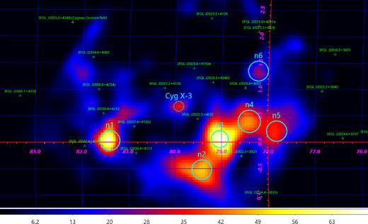
The TS map (Galactic coordinates) at energies ≥1 GeV for the data within a 5° × 5° square around the position of Cyg X-3 with the 3FGL sources subtracted, with their positions marked by the green crosses. The apparently detected sources not present in 3FGL are marked with cyan circles and denoted n1–n6 (see Section 2.1). Cyg X-3 is marked by the dotted cyan circle in the centre.
The spectral analysis in 0.08–300 GeV was performed in a set of narrow energy bins. For each energy bin, we have iteratively removed weak (TS < 1) sources other than Cyg X-3 and then have redone the fit until no weak sources remain.
In addition, we also consider a lower energy band available to the LAT of 40–80 MeV (30–104 MeV accounting for the energy dispersion) for our brightest (flaring) spectrum, where we find an upper limit. For that energy range, we employ a method similar to that used in Zdziarski et al. (2017). This range is not covered by the standard templates for Galactic and isotropic diffuse emission. Therefore, we base our analysis for the Galactic background on three different templates, SLZ6R20T∞C5 , SSZ4R20T150C5, and SYZ6R30T150C2 , produced with the GALPROP code (Vladimirov et al. 2011). Those templates are known to describe Fermi/LAT data at higher energies reasonably well (Ackermann et al. 2012). The spectrum of the standard isotropic background model is available down to 34 MeV, which almost covers the analysed energies, and we employ a power-law continuation of that spectrum down to 30 MeV. We also use a low-value zenith angle cut of zmax = 70°, instead of the standard value of 90° (which we adopt at higher energies).
We have then performed timing analysis for Cyg X-3 in 1-d bins in a broad energy range of 0.1–10 GeV in a way similar to the above-described binned spectral analysis with iterative elimination of weak sources. Fig. 2(a) shows the 1-d bin light curve of the LAT detections. We find 486 d with the signal-to-noise ratios (SNR) >1 and 174 d with SNR >2. The detections with TS ≥16 and <16 are plotted in blue and cyan, respectively. We confirm most of the previous detections by the LAT and AGILE (FLC09; Tavani et al. 2009b; Williams et al. 2011; Bulgarelli et al. 2012; Corbel et al. 2012; Piano et al. 2012; Bodaghee et al. 2013; Cheung & Loh 2016; Loh et al. 2016b; Piano et al. 2016, 2017a,b; Loh & Corbel 2017a,b), which we show by the grey vertical lines. We also find a number of new detections. We then split the days with detections into two energy flux regions, the high-flux region which we call the flaring state and the other, with detections at lower fluxes. The boundary between the two regions, Fb, is selected with the iterative procedure defined as following. At each iteration, we define the mean level Flow and the standard deviation σlow of all detections defined as non-flaring at the previous iteration. If any, we mark all detections with a flux higher than Fb = Flow + 3σlow as flares and continue to the next iteration. The iterations stop when no new detections are attributed to the flaring state. Using this procedure, Fb is found to equal 4.94 × 10⁻¹⁰ erg cm−2 s−1, which is shown by the red horizontal line in Fig. 2(a). We find 49 d with the energy flux ≥ this limit, and we list them in Table 1.
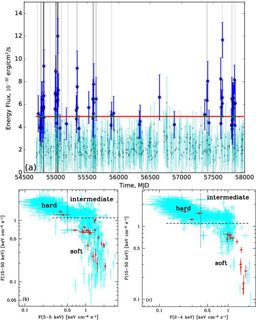
(a) The 1-d bin γ-ray light curve with detections by the LAT. Our criterion defining the flaring state for 1-d integration, F(0.1–100 GeV) > 4.94 × 10⁻¹⁰ erg cm−2 s−1, is shown by the red line. The grey vertical lines correspond to the previously published detections. The large blue circles and small cyan circles with flux error bars correspond to the days with TS ≥16 and <16, respectively. (b) The relationship between the daily-averaged energy fluxes in the 3–5 keV (ASM) and 15–50 keV (BAT) ranges. The hard and soft states are defined here by F(3–5 keV) < 0.5 keV cm−2 s−1 (corresponding to the count rate ≲ 2.7 s−1) and F(15–50 keV) < 1.1 keV cm−2 s−1 (corresponding to the count rate ≲ 0.028 cm−2 s−1), respectively. These boundaries are marked by the dotted and dashed lines, respectively. The intermediate state corresponds to both the 3–5 keV and 15–50 keV fluxes above the respective boundaries. Only points with statistical significance >3σ (required for each of the fluxes) are shown. The thick red circles with error bars correspond to MJDs with LAT flares, defined as above. (c) The same except that the 2–4 keV flux from MAXI is used. The adopted hard-state condition (the dotted line) is here F(2–4 keV) < 0.4 keV cm−2 s−1 (corresponding to the photon flux ≲0.14 cm−2 s−1).
The MJD days corresponding to the flaring state defined in Section 2.1 and Fig. 2(a), with Fγ(0.1–|$100\, {\rm GeV})>4.94\times 10^{-10}$| erg cm−2 s−1. The γ-ray flux and the TS are averages over a given MJD, and the letters S, I, and H correspond to the soft, intermediate, and hard state, respectively.
| MJD | Fγ [10−10 erg cm−2 s−1] | TS | State |
|---|---|---|---|
| 54725 | 5.2 ± 1.6 | 18.5 | H |
| 54780 | 5.7 ± 2.3 | 22.7 | S |
| 54781 | 5.5 ± 1.5 | 23.3 | S |
| 54786 | 6.4 ± 1.6 | 35.3 | S |
| 54809 | 5.8 ± 1.3 | 36.8 | S |
| 54810 | 5.7 ± 1.4 | 32.3 | S |
| 54812 | 9.4 ± 1.4 | 83.0 | S |
| 54814 | 6.8 ± 1.3 | 50.4 | S |
| 54991 | 5.6 ± 1.6 | 18.5 | S |
| 54995 | 7.0 ± 2.2 | 29.0 | S |
| 55002 | 8.9 ± 1.4 | 67.0 | S |
| 55003 | 6.8 ± 1.5 | 43.8 | S |
| 55023 | 6.3 ± 1.2 | 39.9 | S |
| 55032 | 7.0 ± 1.8 | 28.2 | S |
| 55034 | 12.0 ± 1.5 | 119.2 | S |
| 55035 | 6.4 ± 2.1 | 38.7 | S |
| 55043 | 7.2 ± 1.5 | 40.4 | S |
| 55328 | 5.5 ± 1.3 | 29.5 | S |
| 55341 | 5.7 ± 1.3 | 28.4 | S |
| 55342 | 9.2 ± 1.5 | 61.5 | S |
| 55343 | 7.5 ± 1.6 | 38.7 | S |
| 55526 | 5.7 ± 1.4 | 24.8 | H |
| 55592 | 6.5 ± 1.3 | 40.0 | S |
| 55596 | 6.5 ± 1.7 | 31.1 | S |
| 55600 | 5.2 ± 2.1 | 17.6 | S |
| 55604 | 7.8 ± 1.8 | 37.2 | S |
| 55605 | 6.2 ± 1.9 | 23.9 | S |
| 55642 | 6.5 ± 1.9 | 40.5 | S |
| 55888 | 5.0 ± 1.2 | 29.6 | I |
| 55921 | 5.2 ± 1.5 | 19.0 | H |
| 56649 | 6.6 ± 2.0 | 19.3 | H |
| 56766 | 6.1 ± 2.2 | 11.5 | I |
| 57367 | 5.1 ± 1.4 | 19.7 | S |
| 57402 | 6.4 ± 1.4 | 34.0 | S |
| 57414 | 8.0 ± 1.8 | 37.3 | S |
| 57621 | 8.2 ± 1.9 | 35.9 | S |
| 57631 | 5.8 ± 1.5 | 24.4 | S |
| 57646 | 6.1 ± 1.2 | 39.0 | S |
| 57647 | 6.6 ± 1.6 | 41.0 | S |
| 57649 | 11.7 ± 1.5 | 108.6 | S |
| 57799 | 6.5 ± 1.9 | 42.3 | S |
| 57805 | 5.5 ± 1.3 | 35.0 | S |
| 57810 | 6.3 ± 1.6 | 35.7 | S |
| 57816 | 5.7 ± 1.4 | 32.0 | S |
| 57818 | 6.0 ± 1.7 | 42.9 | S |
| 57825 | 6.6 ± 1.4 | 46.3 | S |
| 57826 | 6.2 ± 1.5 | 31.7 | S |
| 57839 | 8.2 ± 1.3 | 63.1 | S |
| 57852 | 6.1 ± 2.0 | 15.9 | S |
We then divide the available LAT observations into the hard, intermediate, and soft states based on the daily-averaged data from All-Sky Monitor (ASM; Bradt, Rothschild & Swank 1993; Levine et al. 1996) on board Rossi X-ray Timing Explorer, the Monitor of All-sky X-ray Image (MAXI; Matsuoka et al. 2009) on board International Space Station, and the Burst Alert Telescope (BAT; Barthelmy et al. 2005; Markwardt et al. 2005; Krimm et al. 2013) on board Swift. The long-term light curves from those detectors are given in ZSP16, and they are updated in Fig. 3. In order to determine the states, we use a method similar to that in Zdziarski et al. (2012a) and in ZSP16, except that we use here the public 15–50 keV BAT data3 instead of custom data used in those papers. We convert the ASM and BAT count rates and the MAXI photon fluxes into energy fluxes using the scaling to the Crab, assuming its spectrum as given in ZSP16. Figs 2(b–c) shows the BAT flux versus the 3–5 keV ASM and 2–4 keV MAXI fluxes. The flux regions delineating the states are defined by the dashed lines. The 3–5 keV boundary of the hard state corresponds to the maximum flux with a positive correlation with the radio emission (ZSP16) and the hard/soft X-rays anti-correlation, and the 15–50 keV boundary approximately corresponds to the lowest fluxes of the hard state. For days without both soft and hard X-ray data, we interpolate the available X-ray data to infer the spectral state, as well as use the 15-GHz data and the radio/X-ray correlations as given in ZSP16. This yields 3074, 736, and 446 d with LAT coverage in the hard, intermediate, and soft state, respectively.
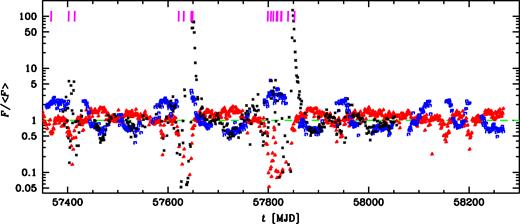
The recent light curves of Cyg X-3 normalized to the respective average over the total observation length. The blue squares, red triangles, and black crosses show the rates normalized to the averages over all available data for the MAXI (2–10 keV), BAT (15–50 keV) and AMI (15 GHz), equal to 0.37 cm−2 s−1, 0.0338 cm−2 s−1, 0.104 Jy, respectively. Only points with the significance ≥2σ are shown; for clarity of display, the error bars are not plotted. The dashed green line corresponds to the averages. The heavy magenta vertical lines correspond to the flares of HE γ-ray emission, as defined in Section 2.1. We note that the last days of the HE γ-ray and 15-GHz data analysed in this work are MJD 57982 and 58055, respectively.
Then, we find 43, 2, and 4 d with γ-ray flares (defined as above) in the soft, intermediate, and hard state, respectively. The points corresponding to the flares for the days with both soft and hard X-ray coverage are shown in red in Figs 2(b–c). They show the four flaring days in the hard state, where one point appears on both panels, i.e. it has both simultaneous ASM/BAT and MAXI/BAT coverages. The occurrence of the intermediate state for two flares was determined by interpolating the X-ray data (see above); thus, those days do not appear in Figs 2(b–c). We see that while most of the days with strong γ-ray detections correspond to the soft state, there are still several detections during the intermediate and hard states, i.e. with low soft X-ray energy fluxes and high hard X-ray ones.
2.2 The radio data
We study here radio-monitoring data at 15 GHz from the Ryle Telescope, which cover MJD 49231–53905 (74181 measurements), and the AMI, MJD 54612–58055 (5125 measurements). The combined data set contains 79306 measurements. The AMI Large Array is the re-built and reconfigured Ryle Telescope. Pooley & Fender (1997) describe the normal operating mode for the Ryle telescope in the monitoring observations; the observing scheme for the AMI Large Array is very similar. The new correlator has a useful bandwidth of about 4 GHz (compared with 0.35 GHz for the Ryle), but the effective centre frequency is similar.
In order to establish the calibration parameters of the array, we use observations of a bright, nearby unresolved source interleaved with those of the main target source. Our primary calibrators were 3C 48 and 3C 286. This procedure resulted in variations in the flux calibration limited to |${\lt}10$| per cent from one day to another.
Throughout this work, we consider the radio emission as coming from the source associated with the accretion/outflow associated with the compact object, presumably the jet. Still, some contribution to that emission comes from the stellar wind. However, it has to be minor, given the very low radio flux levels the source achieves. Another possible contribution is from the stellar wind interacting with disc winds (Koljonen et al. 2018). In this work, we will not distinguish this contribution from the jet, given that we have only 15-GHz radio fluxes at our disposal.
3 LAT SPECTRA IN DIFFERENT STATES
We have calculated the average LAT spectra in the hard, intermediate, soft, and flaring states, as defined in Section 2.1, except that we have excluded the flaring days from the soft-state spectrum. Our results are shown in Fig. 4.
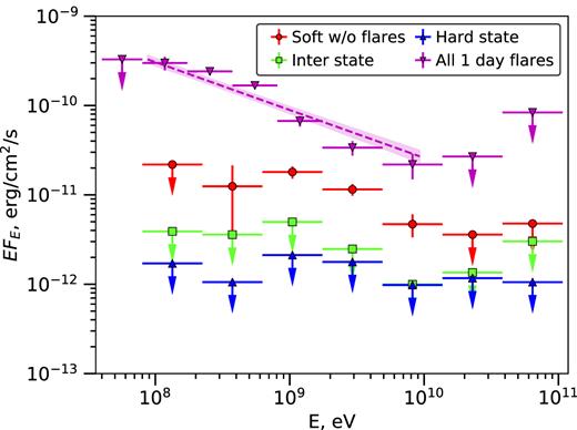
The Fermi LAT spectra and upper limits for the sum of all single MJDs with strong γ-ray detections (the flaring state, as defined in Fig. 2(a), and the soft (excluding the flaring days), intermediate, and hard states, shown by the magenta inverted triangles, red circles, green squares, and blue triangles, respectively, with associated error bars and arrows indicating upper limits. The dashed line and the shaded region show the best power-law fit to the flaring-state spectrum and its uncertainties.
We have detected the source with the significance of ∼40σ during the flaring state in the 0.08–15 GeV range. A power-law fit of the 0.08–10 GeV range gives a photon spectral index of Γ = 2.55 ± 0.05 at the normalization at 100 MeV of 1.9 ± 0.2 ×10⁻⁸ MeV−1 cm−2 s−1, which corresponds to the energy flux above100 MeV of 5.5 × 10⁻¹⁰ erg cm−2 s−1. This power-law spectrum is significantly more accurately determined and slightly harder than the Γ = 2.70 ± 0.25 of FLC09 (measured during MJD 54750–54820 and 54990–55045), and the integrated energy flux is slightly larger than their value of 4.0 ± 1.6 × 10⁻¹⁰ erg cm−2 s−1 at their best fits. Nevertheless, both Γ and the flux are consistent with the FLC09 values within the uncertainties.
However, there is a visible curvature in the present flaring-state spectrum, and we have also fitted it by a lognormal distribution in the form of |${\rm d}N/{\rm d}E=N_0 (E/ E_{\rm b})^{-2} 10^{-\beta \log ^2_{10}(E/E_{\rm b})}$|, where Eb is the peak of it in EFE. (Note that this form is equivalent to a parabola in logarithmic coordinates, see Zdziarski et al. 2016a.) We obtainEb = 384 ± 15 MeV, β = 0.351 ± 0.005, and N0 = 1.36 ± 0.09 × 10⁻⁹ cm−2 s−1. We find that the lognormal/logparabola fit is strongly preferable to the power-law fit, with Δχ2 ≃ −59 for adding one free parameter, which corresponds to a significance of σ ≃ 7–8 of the presence of a curvature. We note that the lognormal model is sharply cut off at |$\gt$|2 GeV and it is thus much below the last detected spectral point.
We still detect Cyg X-3 in the soft state outside the flaring days in the 0.2–15 GeV range at a lower flux than that in the flaring state. This spectrum is parallel to the flaring state one above ∼1 GeV, but we see a hardening at lower energies. We do not detect the source in the intermediate state. Contrary to our original expectations (see Section 1), we have not detected Cyg X-3 in the hard state, obtaining stringent upper limits.
Fig. 5 shows the flaring-state spectrum together with the average X-ray spectra of Cyg X-3 from RXTE (Szostek et al. 2008). In their classification, the average spectra correspond to five spectral states from the hardest to the softest. We have compared our flaring-state spectrum to the models of Zdziarski et al. (2012b), in which relativistic electrons Compton-upscatter blackbody photons emitted by the donor, and which take into account the full Klein–Nishina cross section. Among those, the model with the steady-state electron power-law index of p = 3.5, the minimum electron Lorentz factor of γ1 = 1300, the maximum one of γ2 → ∞, and scattering stellar blackbody photons at the temperature of 105 K, fits well the current spectrum with Δχ2 ≃ −23 with respect to the above power-law fit. Only the normalization has been fitted, yielding the flux at 1 GeV of EFE ≃ 0.0638 keV cm−2 s−1. The Lorentz factor of γ1 corresponds to the minimum above which the electrons are accelerated with an index of pacc ≃ 2.5. Below γ1, the electrons are from cooling by the Compton and adiabatic losses and have the distribution given by equation (21) of Zdziarski et al. (2012b). The electron spectral index is harder than that corresponding to Compton scattering in the Thomson limit, p = 2Γ − 1 = 4.1 because of the Klein–Nishina decline of the Compton cross section, which softens the spectrum. The model satisfies the constraint obtained by Zdziarski et al. (2012a) that the contribution of the jet emission at ∼100 keV is minor (based on the pattern of the orbital modulation found at 50–100 keV). We confirm the result of Zdziarski et al. (2012b) that the magnetic field strength in the γ-ray-emitting region is relatively weak, B ≲ 100 G.
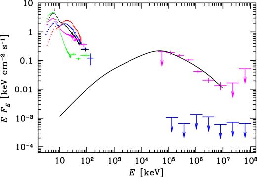
The Fermi LAT measurements and upper limits in the flaring state (upper γ-ray error bars) and the upper limits in the hard state (lower γ-ray error bars) compared to the average RXTE spectra of Cyg X-3 in the five spectral states of Szostek et al. (2008). The X-ray hard-state spectra are the red and blue ones, i.e. with the two top fluxes at 20 keV and bottom at 4 keV, and the remaining spectra correspond to our intermediate and soft states. The solid curve shows the Compton-scattering model spectrum from Zdziarski et al. (2012b) with the electrons with a power-law distribution with the index of p = 3.5 above the low-energy break at γ1 = 1300 and extending up to γ2 → ∞. The electrons scatter stellar blackbody photons with the temperature of 105 K. The fitted normalization is larger by a factor 2.1 than that of Zdziarski et al. (2012b).
Fig. 5 also shows the hard-state spectrum upper limits. We can see that they are quite stringent, implying any jet emission in that state to have an EFE spectrum at a level a few thousand times below the peak of the hard-state X-ray spectrum. We note that the hard-state HE γ-ray spectrum of Cyg X-1 is actually about four orders of magnitude below the peak of the hard-state spectrum (Zanin et al. 2016; Zdziarski et al. 2017). So a γ-ray spectrum at a similar relative level could still be emitted by Cyg X-3 and remain undetectable.
4 ORBITAL MODULATION
4.1 The ephemeris
The above ephemeris is given in the Terrestrial Time MJD and is based on X-ray light curves taking into account the barycentric correction (Y. Bhargava, private communication). Thus, we consider the same time format and apply the barycentric correction to the light curves used for the orbital modulation. In order to determine the orbital phase of a measurement at a time T, we solve equation (1) for n treating it as a real number and then subtract its integer part.
4.2 Modulation of HE γ-rays
We clearly detect the period of Cyg X-3 in HE γ-rays in the flaring state. We note that the orbital period of Cyg X-3 is increasing, which could shift and smear out the peak due to the periodicity. To account for that, we convert the observation time to that of a constant period by calculating n(T) for an observation time, T, by treating n as a real number and solving the binomial in equation (1). We then subtract c0n2 from the time of an observation. The results of our Lomb–Scargle analysis for the light curve corrected in this way are shown in Fig. 6. We find the period of 0.199688(4) d, which, given its standard deviation, agrees very well with P0 of Cyg X-3 of equation (2). We have also found an analogous result on the direct flaring-state light curve, with the peak corresponding to the range of the orbital period during the epoch of the LAT observations, though with a lower peak power, reflecting a period change during that epoch.
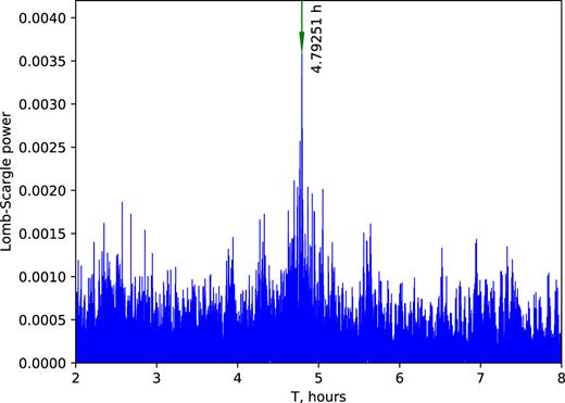
The Lomb–Scargle periodogram for Cyg X-3 in the flaring state in the 0.1–100 GeV range, calculated accounting for the orbital period increase, taking into account the measurement uncertainties, and normalized with the χ2 of a constant model (which results in the power within the 0–1 range). The highest peak corresponds to the orbital period of Cyg X-3.
We then use the ephemeris of Section 4.1 to assign the phase to each photon observed within the ROI during the flaring state and split the data over six equal phase bins. We perform the binned likelihood analysis (see Section 2.1) in each of the bins.5 The resulting energy fluxes as a function of the orbital phase are shown in Fig. 7. We have not found any statistically significant dependence on the energy range, which we looked for by using the photon energy ranges of 0.1–1, 1–10, and 10–100 GeV. We have also verified the consistency of our analysis by checking that the light curve of the nearby pulsar PSR J2032+4127 remains constant in all considered phase bins.
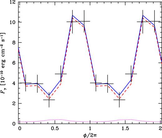
The observed orbital modulation in the flaring state in the 0.1–100 GeV range shown by the error bars. The zero phase is defined from X-rays (Bhargava et al. 2017) and it approximately corresponds to the superior conjunction. For clarity, hereafter two full phase ranges are shown. The blue solid line shows the best fit of the Compton-anisotropy model, and the red dashed and magenta dotted lines show the contributions of the jet and counterjet, respectively.
We then model the orbital light curve obtained by Compton anisotropy. This method utilizes two features of Compton scattering of stellar emission by relativistic electrons. First, the scattering probability is maximized for head-on collisions, i.e. for electrons moving towards the star. Second, a relativistic electron emits the scattered photon predominantly along its direction of motion. Thus, most of the Compton-scattered emission is towards the star and almost no emission is directed to an observer located along the line connecting the star centre and the γ-ray source. Therefore, the observed emission is maximized when the γ-ray source is behind the star. For a jet perpendicular to the orbital plane, this would be at the superior conjunction, and the modulation would be symmetric around it. Departures from that indicate that the jet is inclined with respect to the binary axis.
We use the method of Dubus et al. (2010), including minor corrections given in Zdziarski et al. (2012b), and use the coordinate system shown in Fig. 8 (in which ϕ = 0 corresponds to the superior conjunction). We assume the blackbody photons to be emitted by a point source with the luminosity of |$L_*=4\pi R_*^2\sigma _{\rm B} T_*^4$|, where R* and T* are the stellar radius and temperature, respectively. We also assume the γ-ray source to be a point source, located at a distance, H, from the centre of the compact object. We assume the Thomson limit of Compton scattering, see equation (A9) of Zdziarski et al. (2012b). We take into account the emission of both the jet and counterjet and exclude fits to the observed modulation in which the counterjet is obscured by the star. We calculate the power injected into the non-thermal electrons in the jet+counterjet with a power-law distribution with the index of p = 4.1 (corresponding to the fitted power-law index in the Thomson limit, p = 2Γ − 1) and the minimum Lorentz factor of γmin = 103. We assume fast cooling and thus that power equals the Compton-scattered luminosity emitted by the jet in all directions. In the calculations, we assume the donor mass of M* = 14M|$\odot$|, Mc = 4.5M|$\odot$| (yielding the separation of d = 2.65 × 1011 cm) and the orbital inclination ofi = 31°, which correspond to the solution with the largest allowed masses in Zdziarski et al. (2013). We also assume no eccentricity, R* = 1011 cm, T* = 105 K, and D = 7 kpc. The assumed stellar radius is less than the Roche lobe radius, ≃1.16 × 1011 cm (for the assumed masses; Eggleton 1983).
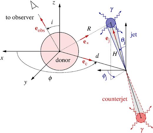
The geometry of Compton scattering of the blackbody photons. The axes x and y are in the binary plane, and the +z direction gives the binary axis. The +x direction gives the projection of the direction towards the observer onto the binary plane. The observer is at an angle, i, with respect to the orbital axis, ϕ is the orbital phase, ϕ = 0 and |$\pi$| correspond to the superior and inferior conjunction, respectively, θj is the inclination of the jet with respect to the binary axis, ϕj is the angle of the projection of the jet onto the binary plane with respect to x-axis, d is the distance between the stars, H is the distance of the γ-ray source from the centre of the compact object, the vectors eobs, ec, and e* point from the donor towards the observer, the centre of the compact object, and the γ-ray source, respectively, and ej points from the centre of the compact object towards the γ-ray source.
Our best-fitting solution, shown in Fig. 7, gives the jet velocity of β ≃ 0.73, the location of the γ-ray source along the jet at H ≃ 6.1 × 1011 cm (≃2.3d), and the jet inclination with respect to the orbital axis of θj ≃ 37°, with an azimuthal angle ϕj ≃ 5° (Fig. 8). Hence, the jet direction is ≃6° off from the line-of-sight, i.e. the jet is nearly pointed towards us. The total χ2 of the fit is 1.35 (with six orbital flux measurements and five fitted parameters, including normalization to the flux). The power injected into the non-thermal electrons (and/or e± pairs) is ≃3.1 × 1036 erg s−1, and the energy content of the electrons is ≃1.1 × 1038 erg. In most of the acceptable solutions, the injected power is between 1036 and 1037 erg s−1. Fig. 9 shows the mutual dependences between θj and ϕj, and βj and H/d. We generally find that the jet has to be inclined with respect to the binary axis by a relatively large angle, θj ≳ 25°, with the γ-ray emission zone located far from the compact object at H ≳ d. The acceptable ranges of our solutions are significantly narrower than those of Dubus et al. (2010) but still consistent with them.
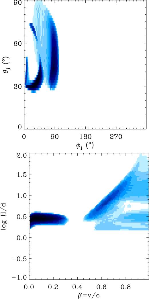
The distributions of the mutual dependences of the found acceptable parameters (within 68 per cent confidence region), ϕj versus θj (top panel), and H/d versus β (bottom panel), obtained with the Compton-anisotropy model applied to the observed γ-ray orbital modulation. The colour changes from white to dark blue |$\propto \sqrt{n}$|, where n is the number of acceptable models per unit area.
We see no evidence for precession within the epoch of the studied LAT observations in either the power spectrum or by comparing the modulation shape at various epochs. It is likely that the inclined jet is aligned with the black hole spin axis up to the location of the γ-ray emission. Occasional jet precession observed in radio (Mioduszewski et al. 2001; Miller-Jones et al. 2004) occurs at much larger distances. If the γ-ray-emitting jet precesses, the obtained parameters correspond to the average orbital modulation. Still, the observed large modulation amplitude, of ∼70–80 per cent, indicates that the precession does not lead to its substantial reduction.
4.3 Modulation of radio emission
We expect to find some orbital modulation of the radio emission in Cyg X-3 caused by free–free absorption in the stellar wind. It is seen, e.g. in the BH HMXB Cyg X-1, where it is strong, with the total amplitude of ≃30 ± 1 per cent at 15 GHz (Zdziarski 2012).
We note, however, that the radio observations of Cyg X-3 have been performed with the visibility window repeating each sidereal day, Ts = 0.99726957 d. Although the observations were scheduled at times determined by the current collection of other requests for observing, and their priorities, the presence of the visibility window results in a strong peak of the power spectrum around 1 d. In addition, harmonics appear, including the fifth one, which is very close to the orbital period. This has apparently prevented any detection of an orbital modulation of the radio emission in spite of many years of observations available. Indeed, we also do not find a significant peak at the orbital period in the power spectrum of the barycentre-corrected light curve. This is shown in Fig. 10(a), where we see a strong broad peak around 1 d, and the peak around the orbital period is seen at a much lower power. The overall maximum power is at 85.95 d.
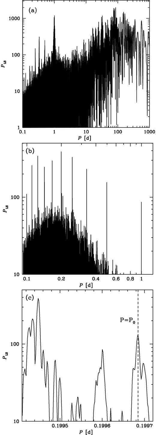
(a) The Lomb–Scargle power spectrum (normalized as in Press et al. 1992) of the barycentre-corrected 15-GHz light curve from the Ryle and AMI telescopes obtained for lnFν. (b) The power spectrum after renormalizing Fν to their running averages over ±0.1 d and transforming the time axis to that corresponding to the constant orbital period. (c) The same as in (b) but zoomed to the region containing both the orbital period, P0 (marked by the dashed line), and the strongest peak.
Thus, in order to see the orbital modulation in the power spectrum, we follow a technique used in Zdziarski et al. (2012a) for calculating folded light curves. In it, we normalize each flux density to its running linear average, see equation (4) in Zdziarski et al. (2012a), determined in the present case by averaging the flux using the observations within ±δ/2 = 0.1–0.2 d of its time (i.e. within 1–2 orbital periods) and requiring at least five observations with the positive fluxes in each average. This reduces the number of usable observations by only 4 per cent, and the average number of observational points used for a renormalized flux is 26 ± 13 for δ = 0.2 d and 37 ± 24 for δ = 0.4 d. We note that this technique corresponds to imposing a high-pass filter in the frequency domain, i.e. it strongly reduces the variability on time-scales longer than the orbital period (very significant in Cyg X-3), thus allowing us to detect the orbital modulation. We also convert the light curve to one corresponding to a constant orbital period in the same way as applied to the γ-ray light curve, see Section 4.2 above. The power spectrum of the resulting light curve is shown in Fig. 10(b). We see that now the strongest peak is around 0.2 d. We show a zoom of the periodogram to the vicinity of P0 in Fig. 10(c), in which we see that we clearly detect the orbital period of P0 = 0.19968476(3) of equation (2), with PLS ≃ 130.
On the other hand, we also see that the strongest peak of the periodogram is at PLS ≃ 390 at a period of ≃0.19944848 d, clearly different from P0. We have searched for the origin of that peak and found that it corresponds to the fifth harmonic of the sidereal day. In order to clearly see it, we have considered the 15-GHz light curve without the barycentric and |$\dot{P}$| corrections. However, we still imposed our high-pass filter with ±δ/2 = 0.1, in order to see variability on time-scales comparable to the orbital period. We have performed the timing analysis on this light curve using both the periodogram and the period-dispersion minimization (PDM; Stellingwerf 1978) method. We show here the results only for the PDM analysis, with those from the periodogram being completely consistent with the PDM ones. Among others, we have found distinct minima of the PDM statistic, θPDM, at Ts, Ts/2, Ts/3, Ts/4, and Ts/5, as shown in Fig. 11(a). A zoom to the region of Ts/5 and P0 is shown in Fig. 11(b). We see that the strongest peak seen in Fig. 10(c) corresponds (after removing the time corrections) exactly to Ts/5. We have also checked that the period observed in HE γ-rays is equal to P0 and that no additional peaks appear in its vicinity, as shown in Fig. 12, which is consistent with the γ-ray observations being performed from space, thus not affected by the daily visibility window.
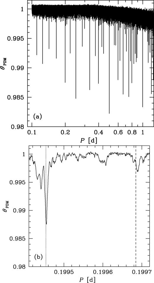
(a) The results of the PDM analysis of the 15-GHz light curve without both the barycentric correction and the correction for the period increase but after renormalizing Fν to their running averages over ±0.1 d, shown for the range of trial periods of 0.1–1.25 d. (b) The same as in (a) but zoomed to the region containing both the orbital period, P0, and the 1/5th of the sidereal day, Ts, marked by the dashed and dotted line, respectively. The seen displacement of the former minimum from the exact value of P0 is due to the correction for |$\dot{P}>0$| not being included in this calculation.
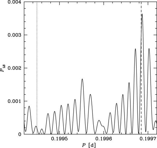
The Lomb–Scargle periodogram for Cyg X-3 in the flaring state in the 0.1–100-GeV range (as in Fig. 6, which takes into account the correction for |$\dot{P}$|) zoomed to the region containing the orbital period (shown by the dashed line) and the strongest peak in Fig. 10(c) (shown by the dotted line).
Therefore, we hereafter consider only the orbital period. We calculate the orbital modulation of the 15-GHz flux by using the light curve renormalized to the running average and take account of the |$\dot{P}$|, as described above. We calculate the average flux and its standard deviation within a given phase bin. We first present our results for the entire (renormalized) radio light curve, which corresponds to the modulation averaged over all flux and spectral states of Cyg X-3, see Fig. 13(a). We see a distinct modulation with a depth of ≃4 per cent.
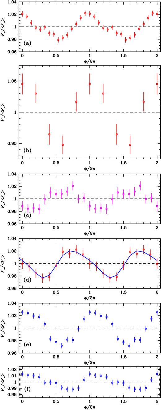
(a) Radio flux folded (using ln Fν) on the orbital period for the entire 15-GHz data renormalized to the local running average (76129). Hereafter, the numbers in parentheses give the respective number of the measurements used. Below, we show the dependences of the orbital modulation on the radio flux range in the soft/intermediate state (b–d) and the hard (e–f) state. We show the results for the data for (b) the lowest soft state (Fν < 30 mJy; 5724); (c) the medium soft state (|$30\, {\rm mJy}\lt F_\nu \le 300\, {\rm mJy}$|, F(3–5 keV) >0.5 keV cm−2 s−1; 14607); (d) the highest soft state (|$F_\nu >300\, {\rm mJy}$|; 8487); (e) the lower hard state (|$30\, {\rm mJy}\lt F_\nu \le 100\, {\rm mJy}$|, F(3–5 keV) < 0.5 keV cm−2 s−1; 8278); and (f) the upper hard state (|$100\, {\rm mJy}\lt F_\nu \le 300\, {\rm mJy}$|, F(3–5 keV) < 0.5 keV cm−2 s−1; 8606). The best fit with the wind-absorption model is shown by the solid line in panel (d).
We then separate the data into subsets based on the radio flux and the X-ray spectral state. Based on fig. 2(b) in ZSP16 and Figs 2(b–c) above, we see that the hard state in Cyg X-3 is characterized by the radio flux density changing in the range of |$30\, {\rm mJy}\lesssim F_\nu \lesssim 300\, {\rm mJy}$| and the 3–5 keV flux of ≲0.5 keV cm−2 s−1. Thus, in order to select the hard state in our data, we use these two criteria for the radio data with available ASM coverage within a day only. Then, the combined soft/intermediate state has the 3–5 keV flux of ≳0.5 keV cm−2 s−1 and the values of the radio flux density anywhere between undetectable flux and 20 Jy, i.e. also including the 30–300 mJy range. We find that there are virtually no measurements with the 3–5 keV flux being <0.5 keV cm−2 s−1 outside the 30–300 mJy range, so we do not need to impose any condition on that flux. Thus, in order to select the soft/intermediate state in our data, we use the radio data with available ASM coverage within a day with the 3–5 keV flux >0.5 keV cm−2 s−1 for the radio data within 30–300 mJy and all the data with Fν < 30 mJy and Fν > 300 mJy.
We show the results for the soft/intermediate state in Figs 13(b–d). We see a significant dependence on Fν. The modulation amplitude is highest for the lowest radio fluxes, with the amplitude of ≃10 per cent, and the modulation extrema are at the phases similar to those for the entire data. Then the intermediate and high fluxes show the amplitudes similar to those for the entire data, ≃4 per cent. There is also a clear shift of the phase of the modulation minima at |$\phi /2\pi \simeq 0.6$|, ≃1.1–1.3, and 1.3–1.4 for the lowest, intermediate, and highest radio-flux range, respectively. Next, we consider the hard state. We also see a significant dependence on Fν, see Figs 13(e–f). The modulation amplitude is higher for the lower range of the flux, 30–100 mJy, with the amplitude of ≃6 per cent, than for the upper range, 100–300 mJy, with the amplitude of ≃2.5 per cent. We also see a shift of the phase of the modulation minima, at |$\phi /2\pi \simeq 0.6$|, ≃0.65–0.85, for the lower and higher radio-flux range, respectively.
The amplitude decrease with the increasing flux within the hard state can be explained by an increase of the height along the jet to where the partially self-absorbed emission becomes optically thin. In the soft/intermediate state, the synchrotron emission is mostly optically thin, but still a larger fraction of the radio flux appears to be emitted close to the compact object for low radio fluxes. Also, the phase of the modulation minimum increasing with the radio flux can be explained by the distance of the location of the bulk of radio emission increasing with the increasing flux and the jet being inclined with respect to the orbital axis. Similar effects are seen in Cyg X-1, see Zdziarski (2012).
The radio orbital modulation and its dependence on the flux can be fitted by the same method and geometry as for γ-rays (Section 4.2) except that now free–free absorption on the wind is included as the modulation process. We assume a constant wind velocity and temperature, vw = 1600 km s−1, Tw = 105 K, respectively, the mass-loss rate by the donor of |$\dot{M}_{\rm w}=7.5\times 10^{-6}{\rm M}_{\odot }$| yr−1 (Zdziarski et al. 2013 and references therein), the He composition (X = 0) and M*, Mc, and i as in Section 4.2. Since the radio emission zone is far from the system, we take into account the effect of the non-zero orbital velocity and finite jet velocity, which can cause a significant change in jet orientation at large distances and a phase delay in the radio modulation. These effects are negligible when fitting the γ-ray orbital modulation.
We fit the orbital modulation averaged over parts of the entire light curve corresponding to the brightest part of the soft state,F > 0.3 Jy (Fig. 13d), since the strong γ-ray emission is observed predominantly in that state and we wish to compare to the jet parameters derived from the γ-ray modulation. We find that the acceptable regions are wide and include values for the jet inclination, θj, and orientation, ϕj, that are compatible with those found for γ-rays, see Fig. 14. Only the location of the 15-GHz source is robustly constrained (by the amplitude of the modulation) to around ∼200d. The best-fitting solution is plotted in Fig. 13(d). The region of dominant 15-GHz emission is located at the distance along the jet ofH ≃ 4.4 × 1013 cm, for a jet velocity of β ≃ 0.45, with θj ≃ 64°, ϕj ≃ 140°, and a total χ2 ≃ 1.9 (10 orbital flux measurements, five fitted parameters). For the best fit, the relative contribution of the counterjet is quite large in the range of 0.33–0.48. A problem with this solution is that it is heavily attenuated, with only a fraction ≃5 × 10⁻⁵ of the intrinsic flux making it to the observer. We note that the average optical depth, 〈τ〉, from the source to infinity is larger by a factor of the order of ∼H/d than the difference in the optical depths between their maximum and minimum values, Δτ (roughly equal to the modulation amplitude), see equations (21–22) in Zdziarski (2012) derived for a perpendicular jet. This explains the large attenuation of this solution.
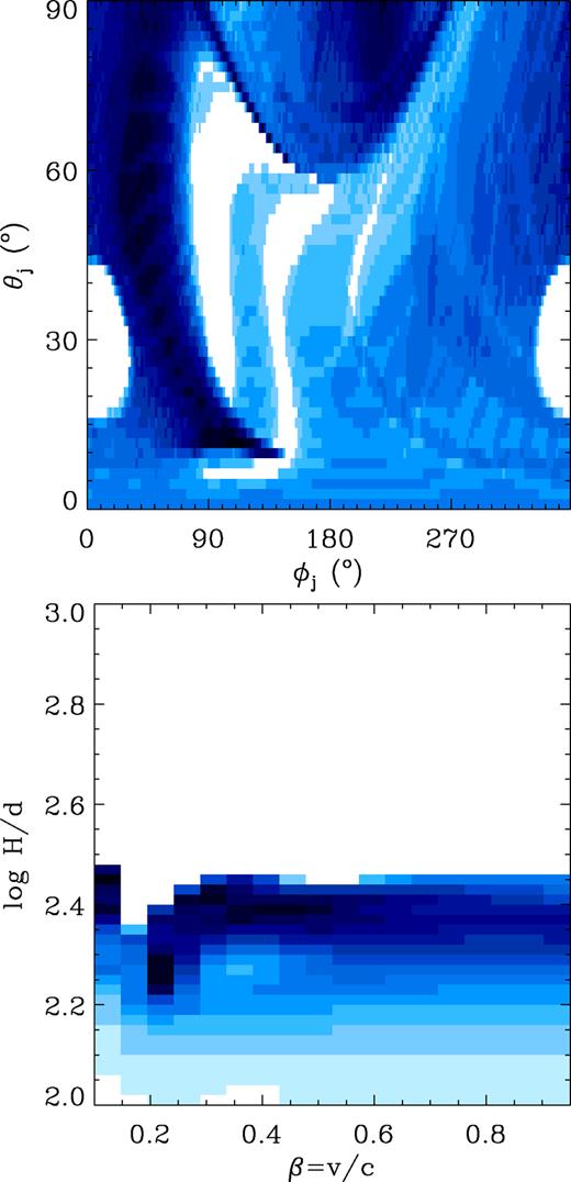
The mutual dependences of the acceptable parameters (within 68 per cent confidence region), ϕj versus θj, and H/d versus β, obtained with the isotropic wind model applied to the observed 15-GHz orbital modulation. The colour changes from white to dark blue |$\propto \sqrt{n}$|, as in Fig. 9.
If we impose the same jet velocity and orientation for both the γ-ray and radio modulation models, we obtain β ≃ 0.55, θj = 30°, and ϕj = 43°, with a total χ2 ≃ 9.5 (with contributions of 5.5 and 4.0 for the γ-ray and radio part, respectively). The locations of the sources are Hγ ≃ 1.1 × 1012 cm and Hr ≃ 4.7 × 1013 cm. The average attenuation of this solution is more moderate, 5.4 × 10⁻².
Finally, we mention that in our investigations we also considered the hypothesis that the strongest peak in Fig. 10(c) is due to a beat with a precession of the jet. The difference of the period of the strongest peak and the orbital period of ≃20 s corresponds to a precession period of ≃170 d (which, interestingly, is about twice the period of the strongest peak in the periodogram of Fig. 10a at ≃86 d). We have then searched for a dependence of the orbital modulation on the precession phase, and, surprisingly, we have found a rather regular dependence on it of both the precession amplitude and the orbital phases of the modulation extrema. Still, the exact coincidence of the found period with the fifth harmonic of the sidereal day convinced us of its origin as an artefact of the visibility window of the radio telescopes. The regular behaviour we found could thus be spurious.
5 CROSS-CORRELATIONS
5.1 The method
This method differs slightly from that of Edelson & Krolik (1988), who considered the values of the standard deviations and the averages for each light curve based on all of their respective points, while here we include only those entering a given bin, as proposed by Lehár et al. (1992). Using global averages and standard deviations can lead to substantial inaccuracies if either a light curve has long-term trends and the cross-correlation is carried over a section of it or it is strongly varying. In particular, we found that the value of the auto-correlation at zero lag is substantially greater than unity in a number of cases considered here. In fact, the value of r is within the range of [−1, 1] only if I′ = J′ = K. Imposing that requires multiple counting (for each occurrence of condition 4) in the mean and standard deviation in cases in which a given xi satisfies condition (4) for more than one yj (or vice versa). Similarly to the case of using global averages and standard deviations, the auto-correlation can exceed unity and the cross-correlation can be not correctly normalized if the multiple counting for the mean and standard deviation is not allowed.
Then, as an option, we average each light curve in the pair within its bin of the size δ before calculating r. This alleviates the above problem of the normalization of r, since then a given xi satisfies condition (4) for (typically) only one value of yj. We have found this to be especially important in the case of correlating the 15-GHz light curve from the AMI with the LAT γ-rays, in which case the LAT light curve has one point per day while the AMI one has typically several. We find then the correlation coefficient with a very noisy dependence on Δt, caused by variations of both the average values and the standard deviations. However, for each shown correlation, we have tested that using different options leads to similar overall shapes of the correlations. Also, we use logarithms of the fluxes, since the flux distributions in Cyg X-3 are much closer to lognormal than to normal (ZSP16), and the calculation of r of equation (3) assumes that the distributions of xi and yi are normal. Lognormal flux distributions have been found in other accreting systems (Uttley, McHardy & Vaughan 2005).
5.2 Cross and auto-correlations in Cyg X-3
We first cross-correlate the γ-ray and radio light curves. We show the results for the LAT detections with the fractional error ≤0.5 within a day (yielding 174 d) in Fig. 15(a) (hereafter the dashed curves show the uncertainty ranges estimated as above). The highest γ-ray fluxes are found in the soft and intermediate states, though we also find a relatively large number of detections in the hard state. The cross-correlation peaks at zero lag, implying that the lag averaged over all frequencies of the variability is <1 d. This is a much more accurate result than the early one of FLC09, who obtained a peak lag of 5 ± 7 d. However, the cross-correlation shows a significant asymmetry, indicating that some radio photons still lag the γ-ray emission by |$\lesssim$|10 d. When the required maximum fractional error is increased, the cross-correlation still peaks at zero lag but becomes weaker, with a lower value of r. We have also considered the case with the radio data split into parts with Fν > 0.3 and <0.3 Jy. For both ranges, the cross-correlations peak at zero lag. Fig. 16(a) shows the relationship between the two daily-averaged energy fluxes on the same MJDs, where we see a positive correlation of the γ-ray flux with the radio one, |$F_{\gamma}\,\, {_{\sim}^{\propto}}\,\,F_{\rm R}^{1/3}$|.
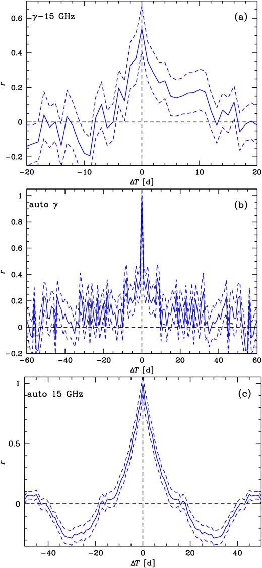
(a) The cross-correlation (solid curve) between the 1-d LAT detections with the fractional error ≤0.5 and the 15-GHz radio emission from the AMI. Hereafter, Δt > 0 corresponds to the signal in the second photon energy range given in the plot label lagging behind the signal in the first range (in the present case, 15-GHz flux lagging the γ-ray one), and dashed curves give the estimated uncertainty range of a correlation. Δt > 0 corresponds to the radio emission lagging the γ-rays. We do not find a measurable lag of the radio emission. (b) The auto-correlation of the γ-ray detections (with the fractional error <1 within a day). (c) The auto-correlation of the 15-GHz emission during the same epoch as that of the Fermi observations.
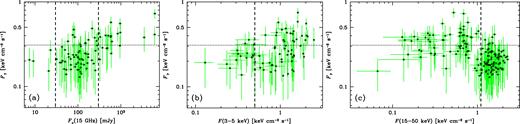
The relationships between the daily 0.1–100 GeV energy fluxes with the fractional error <0.5 and the average of (a) the 15-GHz radio flux, (b) the ASM 3–5 keV flux, and (c) the BAT 15–50 keV flux, on the corresponding MJDs, respectively. The horizontal dotted line gives the boundary of the flaring γ-ray state, and the vertical dashed lines give the boundaries between the hard and soft/intermediate states. In (a), the hard state occurs only between the two dashed lines, but this range also corresponds to the soft/intermediate state. In (b) and (c), the soft state occurs to the right and left of the dashed line, respectively.
The γ-ray emission (all detections with the fractional error <1; 486 d) has a narrow auto-correlation with the width of <1 d, see Fig. 15(b). We also see a weak auto-correlation tail, dropping to null at ≳10 d. On the other hand, the radio emission has a relatively wide auto-correlation, with the half-width at r = 0.5 of 4.5 d, see Fig. 15(c). We then see that the radio emission is anti-correlated with itself for Δt ∼ 30 d. In order to investigate the origin of it, we have split the data set into two parts, above and below 0.3 Jy. We find that the auto-correlation for the low fluxes is similar to the one for all the data, and the ∼30 d time-scale appears to be related to the typical duration of a single occurrence of the hard state. On the other hand, the auto-correlation for the high fluxes is narrower and it becomes negative already at Δt ≃ 8 d and reaches the global negative minimum at 20 d. This appears to be related to the radio flares both preceded and followed by states with weak radio emission (e.g. Szostek et al. 2008).
We then correlate the X-ray and γ-ray emission. Fig. 16(b) shows the correlation with the soft X-rays on the same MJDs. We see that almost all γ-ray detections in the hard state have relatively low fluxes, below the boundary of the flaring state. Then, there is a positive correlation in the soft state. The cross-correlation with soft X-rays is shown in Figs 17(a–b), where the positive correlation at zero lag continues up to a few tens of days, indicating that the γ-ray emission continues after an occurrence of a peak in soft X-rays. This corresponds to occurrences of γ-ray flares during transitions from the softest (hypersoft) X-ray states to harder ones, confirming Koljonen et al. (2010). However, some γ-ray flares also take place during the opposite transitions, which may correspond to weaker peaks at negative lag in Figs 17(a–b),
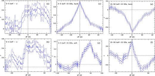
Left-hand panels: The cross-correlation between (a) the 3–5 keV ASM rate and (b) 2–4 keV MAXI rate versus the LAT detections (positive lags correspond to γ-rays lagging the X-rays). Middle panels: The cross-correlation between the 3–5 keV ASM rate in (c) the hard state (FX < 0.5 keV cm−2 s−1, 30 < Fν < 300 mJy) and in (d) the soft/intermediate state (FX > 0.5 keV cm−2 s−1). Right-hand panels: The cross-correlation between the 15–50 keV BAT rate in (e) the hard state (FX > 1.1 keV cm−2 s−1, 30 < Fν < 300 mJy) and in (f) the soft/intermediate state (FX < 1.0 keV cm−2 s−1). Positive lags correspond to radio lagging the X-rays. For all data sets, only data with the fractional error ≤0.5 were considered.
The correlation with hard X-rays is more complicated, see Fig. 16(c). While most of γ-ray detections with high fluxes occur for low hard X-ray flux, i.e. in the soft state, which corresponds to an overall anti-correlation, the detections within the soft state show a weak positive correlation. We also see a large number of detections in the hard state below the boundary of the flaring state. This results in a strong anti-correlation between the γ-ray emission and hard X-rays, with the minimum of the cross-correlation at a lag of γ-rays of ∼5 d (not shown here). However, that lag, given the measurement errors, may be not statistically significant.
We next consider cross-correlations between X-rays and radio in different states. We show the cross-correlations between the softX-rays (3–5 keV) and radio in the hard and soft/intermediate states in Figs 17(c) and (d), respectively. We see that the hard-state relationship gives a strong positive correlation peaking at zero lag (for 1-d bins). The cross-correlation is relatively wide, with a half-width of ∼15 d, and relatively symmetric, showing that some radio photons in the hard state lead and some lag the soft X-rays. We also see some asymmetry at |$|\Delta t|\gt 20$| d, indicating that the lag dominates at long Δt.
On the other hand, while the soft/intermediate state shows almost no correlation at zero lag, it shows a strong positive peak at the radio band delayed by ≃45–48 d, see Fig. 17(d). To investigate it further, we have calculated the relationship between the soft X-ray and radio fluxes in the soft/intermediate state at 0- and 46-d lags. Those plots, not shown here, confirm the lack of a correlation at zero lag changing into a weak positive correlation at the 46-d lag. We note that the 45–48-d lag appears to correspond to the average time spent in the ultra/hypersoft X-ray state that directly precedes major radio flares. For instance, in 2011, the radio emission was quenched for a month while the source was in the ultra/hypersoft state, ending with a major 10-Jy radio flare (Corbel et al. 2012). The interpretation of the physical nature of this lag appears, however, unclear. It may correspond to a time-scale linked to magnetic field rearrangement in the disc so that a jet can be launched. It may also correspond to the propagation time-scale from the centre to the dominant large-scale jet component of the radio emission (at tens of mas; Tudose et al. 2010). This interpretation, however, implies a rather low speed of the jet, ∼0.1c. The radio emission is also seen on arcsec scales, as found by Martí et al. (2001), which may contribute to that long lag as well. We have also calculated the soft X-rays versus 15-GHz cross-correlation without separating into the states to be able to directly compare it to the 3–5 keV versus γ-ray cross-correlation. It shows the shape relatively similar to that of Fig. 17(b), with a positive r at zero lag and a peak below 50 d.
Hard X-rays, 15–50 keV, are anti-correlated with the radio band in the hard state (i.e. for large X-ray fluxes), see Fig. 17(e). There appears to be a 1-d lag of the radio emission here, but it is not statistically significant. On the other hand, the hard X-rays are positively correlated with the radio at zero lag in the soft/intermediate state, see Fig. 17(f). However, they also show an anti-correlation with radio peaking at a lag of ∼30 d; see Fig. 17(f). This behaviour is likely to be related to the 45–48-d lag at soft X-rays, Fig. 17(d).
We then show the auto-correlation functions for the 3–5 and 15–50 keV energy ranges, and their cross-correlations in Figs 18(a–b), respectively. Interestingly, the 15–50-keV auto-correlation is substantially narrower, with the half-width of ≃20 d, than the 3–5 keV one, with the half-width of ≃40 d. This difference may correspond to the hard X-ray emission region being closer to the compact object and thus smaller than that for soft X-rays. On the other hand, it may also correspond to the 15–50-keV emission leading the 3–5 keV one. Interestingly, the widths of the X-ray auto-correlations are of the same order as the radio versus X-ray lags in the soft state, Figs 17(d–f).
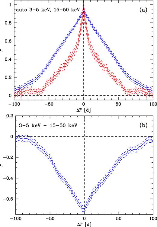
(a) The auto-correlation for the 3–5-keV ASM (upper blue curve) and the 15–50-keV BAT (lower red curve) rates. (b) The cross-correlation between the 3–5-keV and 15–50-keV rates in all states.
We also note that Tudose et al. (2010) argued that the radio/X-ray correlation observed at zero lag (e.g. Szostek et al. 2008) is not theoretically expected in bright radio states, where the bulk of the radio emission is in the jet rather than in the core. However, this does not seem to present a problem, given the projected jet distance from the core of ∼1–2 light days and the widths of the auto-correlations of both radio and X-rays are ≫2 d.
6 CONCLUSIONS
We have obtained the following main results.
Based on 9 yr of the Fermi data, we have searched for occurrences of significant HE γ-ray emission from Cyg X-3. We have found a large number of days with significant LAT detections, and among them, 49 d with the 0.1–100-GeV energy fluxes above the flaring level, which we defined at 4.94 × 10⁻¹⁰ erg cm−2 s−1 based on the level 3σ above the average of non-flaring detections. Out of them, 43 d are in the soft spectral state.
We have calculated the average γ-ray spectrum during strong flares (with positive detections in the 0.08–15-GeV energy range) and the spectrum averaged over all the occurrences of the soft spectral state (detected in the 0.5–15-GeV range). On the other hand, we have found only upper limits in the hard and intermediate states. The flaring-state spectrum is well modelled by Compton scattering of the blackbody photons from the donor by jet relativistic electrons with a power-law distribution with the spectral index of ≃3.5 and the low-energy cutoff at the Lorentz factor of ∼103.
From the LAT data, we have also obtained the profile of the orbital modulation of γ-rays in the flaring state, which is significantly more accurate than the previous one of FLC09. The amplitude of the modulation is large, by a factor of ≃5, and it is well modelled by Compton scattering of stellar blackbody, which agrees with the modelling of the spectrum. The modulation model implies the location of the γ-ray source at the distance along the jet similar to the separation between the binary components, a mildly relativistic jet velocity, and it requires that the jet is inclined at an angle ≳25° with respect to the binary axis.
We have then studied the 22 yr of 15-GHz radio observations of Cyg X-3 by the Ryle and AMI telescopes. We have discovered pronounced modulation of the radio emission at the orbital period. The amplitude of the modulation depends on both the spectral state and the flux level. It changes from ≃2.5 to ≃10 per cent, and it is ≃4 per cent when averaging over all the data. We model the observed modulation as free–free absorption in the stellar wind of the jet radio emission. We find the 15-GHz source to be located at a distance of ∼102 times the binary separation.
Finally, we have studied cross-correlations between the HE γ-ray and radio light curves, as well as between either of them and light curves from the ASM, MAXI, and BAT X-ray monitors. We have found the correlation coefficient between the HE γ-ray and 15-GHz light curves peaks at zero lag. However, its asymmetry indicates that some radio photons lag the γ-rays by |$\lt$|10 d. Then, the γ-rays lag soft X-rays by some tens of days but without showing a clear peak of the correlation coefficient. This is consistent with occurrence ofγ-ray flares mostly during the soft-to-hard transitions. Also, we have not found measurable lags between the X-ray and radio emission in the hard spectral state. On the other hand, we have found the lag peaking at 45–48 d of the 15-GHz emission with respect to 3–5-keV soft X-rays in the soft state. This lag is similar to the time spent in the X-ray ultra/hypersoft and radio-quenched state before a major flare occurs.
ACKNOWLEDGEMENTS
We thank the referee and members of the Fermi LAT Collaboration for valuable comments. This research has been supported in part by the Polish National Science Centre grants 2013/10/M/ST9/00729, 2015/18/A/ST9/00746, and 2016/21/P/ST9/04025, and the Carl-Zeiss Stiftung through the grant ‘Hochsensitive Nachweistechnik zur Erforschung des unsichtbaren Universums’ to the Kepler Zentrum für Astro- undTeilchenphysik at the University of Tübingen, and by the state of Baden-Württemberg through bwHPC. The authors thank the SFI/HEA Irish Centre for High-End Computing (ICHEC) for the provision of computational facilities and support. The Fermi LAT Collaboration acknowledges generous ongoing support from a number of agencies and institutes that have supported both the development and the operation of the LAT as well as scientific data analysis. These include the National Aeronautics and Space Administration and the Department of Energy in the United States, the Commissariat à l’Energie Atomique and the Centre National de la Recherche Scientifique/Institut National de Physique Nucléaire et de Physique des Particules in France, the Agenzia Spaziale Italiana and the Istituto Nazionale di Fisica Nucleare in Italy, the Ministry of Education, Culture, Sports, Science and Technology (MEXT), High Energy Accelerator Research Organization (KEK) and Japan Aerospace Exploration Agency (JAXA) in Japan, and the K. A. Wallenberg Foundation, the Swedish Research Council and the Swedish National Space Board in Sweden. Additional support for science analysis during the operations phase is gratefully acknowledged from the Istituto Nazionale di Astrofisica in Italy and the Centre National d’Études Spatiales in France. This work has been performed in part under DOE Contract DE-AC02-76SF00515. The AMI arrays are supported by the University of Cambridge and by the UK STFC. This research has made use of the results provided by the ASM and BAT teams and MAXI data provided by RIKEN, JAXA, and the MAXI team.
Footnotes
We note that the template of van der Klis & Bonnet-Bidaud (1989) has the minimum slightly below zero phase, which is also the case for the X-ray light curves phase-folded based on a previous ephemeris in Zdziarski et al. (2012a). Furthermore, the strongest X-ray absorption may not exactly correspond to the conjunction due to a likely asymmetry of the stellar wind in this short-period binary.
REFERENCES
Author notes
Present address: Naval Research Laboratory, Washington, DC 20375, USA
