KiDS+2dFLenS+GAMA: testing the cosmological model with the EG statistic

Amon, A; Blake, C; Heymans, C; Leonard, C D; Asgari, M; Bilicki, M; Choi, A; Erben, T; Glazebrook, K; Harnois-Déraps, J; Hildebrandt, H; Hoekstra, H; Joachimi, B; Joudaki, S; Kuijken, K; Lidman, C; Loveday, J; Parkinson, D; Valentijn, E A; Wolf, C

doi:10.1093/mnras/sty1624

ABSTRACT

We present a new measurement of E_G, which combines measurements of weak gravitational lensing, galaxy clustering, and redshift-space distortions. This statistic was proposed as a consistency test of General Relativity (GR) that is insensitive to linear, deterministic galaxy bias, and the matter clustering amplitude. We combine deep imaging data from KiDS with overlapping spectroscopy from 2dFLenS, BOSS DR12, and GAMA and find |$E_{\rm G}(\overline{z}=0.267)=0.43 \pm 0.13$| (GAMA), |$E_{\rm G}(\overline{z}=0.305)=0.27 \pm 0.08$| (LOWZ+2dFLOZ), and |$E_{\rm G}(\overline{z}=0.554)=0.26 \pm 0.07$| (CMASS+2dFHIZ). We demonstrate that the existing tension in the value of the matter density parameter hinders the robustness of this statistic as solely a test of GR. We find that our E_G measurements, as well as existing ones in the literature, favour a lower matter density cosmology than the cosmic microwave background. For a flat ΛCDM Universe, we find Ω_m(z = 0) = 0.25 ± 0.03. With this paper, we publicly release the 2dFLenS data set at: http://2dflens.swin.edu.au.

gravitational lensing: weak, surveys, cosmology: observations, large-scale structure of Universe

1 INTRODUCTION

Many observations reveal that within the Friedmann–Robertson–Walker (FRW) framework, the Universe is undergoing a late-time, accelerated expansion, which is driven by some unknown ‘dark energy’ (see e.g. Copeland, Sami & Tsujikawa 2006). While a vacuum energy is the simplest and most widely accepted model of dark energy, there exists an enormous discrepancy between its theoretical and observed value (Weinberg 1989). To address this problem, a wide range of alternative models have been proposed including those where gravity behaves differently on large cosmological scales from the framework laid down by Einstein’s General Relativity (GR). As an understanding of the nature of this dark energy phenomenon still evades scientists, it is imperative that current cosmological surveys conduct observations to test for such departures on cosmological scales (Weinberg et al. 2013).

The perturbed FRW space–time metric may be completely defined in terms of the Bardeen potentials (Bardeen 1980), namely the Newtonian potential, Ψ, which along with density perturbations drives the structure formation of the Universe, and the curvature potential, Φ, as well as an expansion scale factor for the Universe, a(t), as

\begin{eqnarray*} {\rm d}s^2 = -c^2{\rm d}t^2(1+2\Psi)+ a(t)^2 {\rm d}\mathbf {x}^2 (1-2\Phi) , \end{eqnarray*}

(1)

where x represents the spatial elements of the metric. While cosmological probes by themselves can be subject to model degeneracies and systematic biases, a combination of probes, specifically using imaging and spectroscopic surveys, can test for departures from GR (see e.g. Zhang et al. 2007; Jain & Zhang 2008). The Bardeen potentials are equal in the absence of anisotropic stress, as in the case of GR. This is not necessarily the case in modified gravity theories (Pogosian & Silvestri 2008), although recent gravitational wave measurements have set tight constraints on these scenarios (Lombriser & Taylor 2016; Baker et al. 2017; Creminelli & Vernizzi 2017; Ezquiaga & Zumalacárregui 2017; Lombriser & Lima 2017; Sakstein & Jain 2017; Amendola et al. 2018).

Weak gravitational lensing, a statistical quantification of the deflection of light by overdensities in the Universe, has proven itself to be a powerful cosmological probe (see e.g. Heymans et al. 2013; Hildebrandt et al. 2017; Troxel et al. 2017). This measurement is sensitive to the curvature potential, ∇²(Ψ − Φ), because relativistic particles collect equal contributions from the two potentials as they traverse equal quantities of space and time. One particular observable, galaxy–galaxy lensing, measures the deflection of light due to the gravitational potential of a set of foreground lens galaxies, rather than the large-scale structure as a whole (Hoekstra, Yee & Gladders 2004; Mandelbaum et al. 2005).

The clustering effect of the non-relativistic peculiar motions of foreground galaxies can be quantified by measuring redshift-space distortions (RSD; Kaiser 1987). The gravity-driven motion produces Doppler shifts in galaxy redshifts that are correlated with each other. As a result, an overall anisotropy is imprinted in the measured redshift-space clustering signal that is a function of the angle to the line of sight. This anisotropy is the redshift-space distortion and an accurate measurement of its amplitude probes the growth rate of cosmic structure, f. These probes are sensitive only to derivatives of the Newtonian potential, ∇²Ψ and as such, in conjunction with the lensing signal due to the foreground lens galaxies, allows us to isolate the relativistic deflection of light from background galaxies. This creates a fundamental test of the relationship between Ψ and Φ.

The complementarity between imaging and spectroscopic surveys has been exploited in the examination of the level of concordance of cosmological measurements from combined lensing, clustering, and/or redshift-space distortion analyses (Joudaki et al. 2018; van Uitert et al. 2018), compared to cosmic microwave background (CMB) temperature measurements from the Planck satellite (Planck Collaboration XIII 2016). These combined-probe analyses (see also DES Collaboration 2017) found varying levels of ‘tension’ with the Planck CMB measurements. In this analysis we combine lensing, clustering, and redshift-space distortion measurements to probe the E_G statistic (Zhang et al. 2007). The relative amplitude of the observables is used to determine whether GR’s predictions hold, assuming a perturbed FRW metric and a defined set of cosmological parameters. Any deviations on large scales from the GR prediction for E_G, which is scale-independent will suggest a need for large-scale modifications in gravitational physics.

As a choice is made for the cosmology used to compute a GR prediction for E_G, this brings into question the use of this statistic to test GR while any uncertainty exists in the values of the cosmological parameters. This is relevant as there exists a current ‘tension’ in the literature between cosmological parameters (specifically |$\sigma _8\sqrt{\Omega _{\rm m}/0.3}$|⁠) constrained by Planck CMB experiments (Planck Collaboration XIII 2016) and lensing or combined probe analyses. More specifically, Hildebrandt et al. (2017) and Joudaki et al. (2018) report a 2.3σ and 2.6σ discordance with Planck constraints. We investigate whether the deviations we find from a Planck GR prediction are consistent with the expectations given by the existing tension between early Universe and lensing cosmologies. Even with this uncertainty, however, the E_G statistic still provides a test of the theory of gravity through its scale dependence. We conduct this test, while investigating the possibility of this effect’s degeneracy with scale-dependent bias.

The power of combined-probe analyses was investigated by, for example Zhao et al. (2009), Cai & Bernstein (2012), and Joudaki & Kaplinghat (2012) and later applied to data (Tereno, Semboloni & Schrabback 2011; Simpson et al. 2013; Zhao et al. 2015; Planck Collaboration XIII 2016; Joudaki et al. 2018). In this paper, we extend the original E_G measurement performed by Reyes et al. (2010) in redshift and scale, using the on-going large-scale, deep imaging Kilo-Degree Survey (KiDS; Kuijken et al. 2015) in tandem with the overlapping spectroscopic 2-degree Field Lensing Survey (2dFLenS; Blake et al. 2016b), the Baryon Oscillation Spectroscopic Survey (BOSS; Dawson et al. 2013), and the Galaxy and Mass Assembly survey (GAMA; Driver et al. 2011). With the combination of these data, we extend the statistic to |${\sim }50 \, h^{-1}$|Mpc in three redshift ranges. Alam et al. (2017), Blake et al. (2016a), and de la Torre et al. (2017) previously probed the same high-redshift range and the latter two cases find some tension between their measurements compared to a Planck cosmology. Pullen et al. (2016) measured E_G with a modified version of the statistic that incorporates CMB lensing and allows them to test larger scales, finding a 2.6σ deviation from a GR prediction, also computed with a Planck cosmology. A number of possible theoretical systematics, as well as predictions for E_G in phenomenological modified gravity scenarios are discussed in Leonard, Ferreira & Heymans (2015a).

This paper is structured as follows. Section 2 describes the underlying theory of our observables. An outline of the various data sets and simulations involved in the analysis is given in Section 3. In Section 4, we present the different components of the E_G statistic and detail how those measurements were conducted, while in Section 5, we provide our main E_G measurement in comparison to existing measurements, as well as to models using different cosmologies and with alternative theories of gravity. We summarize the outcomes of this study and provide an outlook in Section 6.

2 THEORY

2.1 Differential surface density

Galaxy–galaxy lensing can be mathematically expressed in terms of the cross-correlation of a galaxy overdensity, δ_g, and the underlying matter density field, δ_m, given at a fixed redshift by ξ_gm(r) = 〈δ_g(x)δ_m(x + r)〉_x. In order to measure the lensing galaxy–matter cross-correlation function, ξ_gm, one can first determine the comoving projected surface mass density, Σ_com, around a foreground lens at redshift z_l, using a background galaxy at redshift z_s and at a comoving projected radial separation from the lens, R. This is given as

\begin{eqnarray*} \Sigma _{\rm com}(R)= \overline{\rho _{\rm m}} \int _{0}^{\chi (z_{\rm s})} \ \xi _{\rm gm} \big (\sqrt{R^2+[\chi -\chi (z_{\rm l})]^2} \big) \ \rm {d}\chi , \end{eqnarray*}

(2)

where |$\overline{\rho _{\rm m}}$| is the mean matter density of the Universe, χ is the comoving line-of-sight separation, and χ(z_l), χ(z_s) are the comoving line-of-sight distances to the lens and source galaxy, respectively. The shear is sensitive to the density contrast, and therefore it is a measure of the excess or differential surface mass density, ΔΣ_com(R) (Mandelbaum et al. 2005). This is defined in terms of Σ_com(R) as

\begin{eqnarray*} \Delta \Sigma _{\rm com}(R)=\overline{\Sigma }_{\rm com}(\le R) - \Sigma _{\rm com}(R) , \end{eqnarray*}

(3)

where the average projected mass density within a circle is

\begin{eqnarray*} \overline{\Sigma }_{\rm com}(\le R)=\frac{2}{R^2} \int ^R_0 \Sigma _{\rm com}(R^{\prime }) R^{\prime } \rm {d}R^{\prime } . \end{eqnarray*}

(4)

For a sufficiently narrow lens distribution (such that it may be approximated as a Dirac Delta function at z_l), in the context of GR, the physical differential surface mass density of the lens is related to the tangential shear, γ_t, of background galaxies as

\begin{eqnarray*} \Delta \Sigma _{\rm phys}(R) = \gamma _{\rm t}(R)\Sigma _{\rm c, phys} . \end{eqnarray*}

(5)

where Σ_{c, phys} is the critical surface mass density. This is defined as

\begin{eqnarray*} \Sigma _{\rm c, phys}= \frac{c^2}{4\pi G} \frac{D(z_{\rm s})}{D(z_{\rm l}) D(z_{\rm l},z_{\rm s})} , \end{eqnarray*}

(6)

where D(z_s), D(z_l), andD(z_l, z_s) are the angular diameter distances to the source, to the lens, and the angular diameter distance between the source and lens, respectively, G is the gravitational constant, and c is the speed of light. The surface mass density or the convergence, κ, can be expressed as the ratio of the physical projected and critical surface mass densities, Σ_phys and Σ_{c, phys}, respectively, or the equivalent in comoving units, as

\begin{eqnarray*} \kappa = \frac{\Sigma _{\rm phys}}{\Sigma _{\rm c, phys}}= \frac{\Sigma _{\rm com}}{\Sigma _{\rm c,com}} , \end{eqnarray*}

(7)

where the comoving and physical critical surface mass densities¹ for a lens at redshift z_l are related by

\begin{eqnarray*} \Sigma _{\rm c, com}= \frac{\Sigma _{\rm c, phys}}{(1+z_{\rm l})^2} . \end{eqnarray*}

(8)

The cross-correlation of the lens galaxies and the underlying mass, ξ_gm(r), that appears in the definition of the differential surface mass density given by equation (2), depends on the way that the lens galaxies trace their matter field. This is known as the ‘galaxy bias’, b, and it can be stochastic, non-linear, and scale-dependent on small scales (Dekel & Lahav 1999). However, on linear scales, the galaxy overdensity is expected to be related to the matter overdensity as

\begin{eqnarray*} \delta _{\rm g}(\boldsymbol{x})=b \ \delta _{\rm m}(\boldsymbol{x}) , \end{eqnarray*}

(9)

so that

\begin{eqnarray*} \xi _{\rm gm}(r)=b \ \xi _{\rm mm}(r) , \end{eqnarray*}

(10)

where ξ_mm(r) is the matter autocorrelation function, which can be derived from the cosmological model (Kaiser 1984).

2.2 Galaxy clustering: redshift-space distortions

An observed redshift has a contribution from the expansion of the Universe, known as the cosmological redshift, and another from the peculiar velocity. Measurements sensitive to the peculiar velocities of galaxies are a particularly useful tool for testing gravitational physics. Peculiar velocities are simply deviations in the motion of galaxies from the Hubble flow due to the gravitational attraction of objects to surrounding structures.

The two-point statistics of the correlated positions of galaxies in redshift space are a powerful tool for testing GR growth predictions (Guzzo et al. 2008). Large-scale clustering in real space is isotropic. However, redshift-space distortion introduces a directional dependence such that the redshift-space power spectrum under the assumption of linear theory is

\begin{eqnarray*} P_{\rm gg} (k,\eta)= b^2(1+ \beta \eta ^2)^2 P_{\rm mm}(k) , \end{eqnarray*}

(11)

where P_mm is the real space matter power spectrum and η is the cosine of the angle of the Fourier mode to the line of sight (Hamilton 1993). The factor β is introduced as a redshift-space distortion parameter which governs the anisotropy of the clustering amplitude on the angle to the line of sight. This factor is defined as

\begin{eqnarray*} \beta \equiv \frac{f(z)}{b(z)} , \end{eqnarray*}

(12)

where f(z) is the growth rate of structure. It can be expressed in terms of the growth factor D₊(a) at a particular cosmic scale factor, a, defined in terms of the amplitude of the growing mode of a matter density perturbation as δ_m(a) = D₊(a)δ_m(z = 0) to give

\begin{eqnarray*} f(z)\equiv \frac{{\rm d} \, \ln D_+(a)}{{\rm d} \, \ln a} . \end{eqnarray*}

(13)

As a function of the matter density parameter, in the absence of anisotropic stress in GR and with a flat Universe, the growth rate is well approximated in terms of the matter density parameter at a given redshift, Ω_m(z), as f(z) ≈ Ω_m(z)^0.55 (Wang & Steinhardt 1998; Linder 2005).

2.3 Galaxy clustering: projected correlation function

Galaxy clustering independent of RSD can be analysed in terms of the projected separation of galaxies on the sky. We call the associated two-point function in real space the ‘projected correlation function’, w_p(R), and it is formulated from the integral of the 3D galaxy correlation function, ξ_gg(R, Π), along the line of sight as

\begin{eqnarray*} w_{\rm p}(R)= \int ^{+\infty }_{-\infty }\xi _{\rm gg}(R, \Pi) \ \mathrm{ d}\Pi , \end{eqnarray*}

(14)

where Π is the co-moving separation along the line of sight.

2.4 Suppressing small-scale systematics

It is evident that the differential surface density of matter, defined in equation (4), includes a range of smaller scales from zero to R. However, the cross-correlation coefficient between the matter and the galaxy fluctuations is a complicated function at scales within the halo virial radius (Cacciato et al. 2012) and furthermore, lensing systematics can dominate on small scales (Mandelbaum et al. 2010). Thus, in order to reduce the measurement’s systematic uncertainty, its sensitivity to small-scale information should be suppressed. This is achieved through a statistic, the comoving annular differential surface density, proposed by Mandelbaum et al. (2010) as

\begin{eqnarray*} \Upsilon _{\rm gm}(R,R_0)= \Delta \Sigma _{\rm com}(R)- \frac{R_0^2}{R^2}\Delta \Sigma _{\rm com}(R_0) , \end{eqnarray*}

(15)

where R₀ is the small-scale limit below which information is erased. The minimum length-scale is chosen to be large enough to reduce the dominant systematic effects, but small enough to maintain a high-signal-to-noise ratio in the galaxy–lens correlation measurement. A similar statistic is formulated in order to remove the small-scale contribution to the galaxy autocorrelation,

\begin{eqnarray*} \Upsilon _{\rm gg}(R,R_0)= \rho _{\rm c} \Big [ \frac{2}{R^2} \int _{R_0}^{R} R^{\prime } w_{\rm p}(R^{\prime })dR^{\prime }-w_{\rm p}(R)+\frac{R_0^2}{R^2}w_{\rm p}(R_0)\Big ], \end{eqnarray*}

(16)

where ρ_c is the critical density.

We note that an alternative method to remove small-scale systematics was introduced in Buddendiek et al. (2016), where they generalized the Υ formalism from Baldauf et al. (2010) by an expansion of the galaxy–galaxy and galaxy–matter correlation functions using a complete set of orthogonal and compensated filter functions. This is inspired by COSEBIs for the case of cosmic shear analysis defined in Schneider, Eifler & Krause (2010) [see Asgari et al. 2017, for an application to data].

2.5 The E_G statistic

The E_G statistic, as proposed by Reyes et al. (2010), is defined as a combination of the annular statistics Υ_gm(R, R₀) and Υ_gg(R, R₀) with the RSD parameter, β (equations 15, 16, 12, respectively) as

\begin{eqnarray*} E_{\rm G}(R)=\frac{1}{\beta } \frac{\Upsilon _{\rm gm}(R,R_0)}{\Upsilon _{\rm gg}(R,R_0)} , \end{eqnarray*}

(17)

where all of the statistics are measured for a particular lens galaxy sample. This measurement depends on the redshift of the lens galaxy sample, z_l, but we omit this for clarity. In this combination, the contribution of a linear galaxy bias, as well as the shape of the matter clustering in the measurements approximately cancel.

The gravitational statistic was initially theorized by Zhang et al. (2007), who proposed it as an estimator of the form

\begin{eqnarray*} \tilde{E}_{\rm G}(l) = \frac{C_{\rm {g} \kappa }(l)}{3 H_0^2 a^{-1}(z) C_{\rm {g} v} (l)}\, , \end{eqnarray*}

(18)

where C_gκ is the projected cross-power spectrum of source galaxy convergence with lens galaxy positions, l is the amplitude of the on-sky Fourier space variable conjugate to projected radius, H₀ is the Hubble parameter today, and C_gv(l) is a projected version of the cross-power spectrum of lens galaxy positions and velocities. The theoretical expectation value of this statistic, averaged over l , is predicted to take the value,

\begin{eqnarray*} E_{\rm G}(z)=\frac{ \nabla ^2[\Psi (z)+\Phi (z)]}{3H_0^2 a^{-1}(z) f(z) \delta _{\rm m}(z)}\, , \end{eqnarray*}

(19)

where δ_m is the matter field overdensity and Ψ(z) and Φ(z) are the Bardeen potentials from equation (1). In this equation, we do not indicate the k-dependences of Ψ, Φ, and δ_m because in linear regime, these cancel, thereby making E_G(z) independent of k. Invoking mass-energy conservation in a standard FRW Universe, and under the assumption that we are in the linear regime, results in Ψ = Φ and

\begin{eqnarray*} \nabla ^2\Phi =\nabla ^2\Psi =\frac{3}{2}\Omega _{\rm m}(z=0)H_0^2a(z)^{-1}\delta _{\rm m}(z) \, . \end{eqnarray*}

(20)

Zhang et al. (2007) showed that this can be reduced to a value of E_G(z) which is a function of the matter density parameter valued today, Ω_m(z = 0), and the growth rate of structure, f(z), that is independent of the comoving scale R and defined to be

\begin{eqnarray*} E_{\rm G}(z)=\frac{\Omega _{\rm m}(z=0)}{f(z)} \, . \end{eqnarray*}

(21)

Here, the dependence of this statistic on an underlying cosmology is evident. As the prediction from GR is scale-independent , it is useful to compress the observable defined in equation(17) to a scale-independent measurement at the effective redshift of the lens sample, |$E_{\rm G}(\hat{z})=\langle E_{\rm G}(R) \rangle$|⁠.

The elegance of the statistic proposed by Zhang et al. (2007) is that it is constructed to be independent of the poorly constrained galaxy bias factor, b, given that on large scales, linear theory applies. However, measuring E_G following equation (18) requires a Fourier space treatment of probes which are typically analysed in real space, as well as a measurement of the cross-spectra of galaxy positions with convergence and velocities, which are in practice challenging to determine directly. The real-space statistic of equation (17) is hence the more convenient estimator and the one we employ in this paper. Leonard, Baker & Ferreira (2015b) showed that in the case of linear bias, a flat cosmology and in GR, |$E_{\rm G}=\tilde{E}_{\rm G}$|⁠. It is worth noting, however, that in real space we lose the ability to cleanly restrict the measurement to the linear regime. Therefore, it is less clear at which scales E_G remains independent of galaxy bias. As shown in Alam et al. (2017) using N-body simulations, this effect is expected to be at most of the order of 8 per cent at 6h⁻¹Mpc for LRGs, and therefore is unlikely to affect our results significantly. We explore the effect of galaxy bias in the measurement in Section 5.

2.6 Modifications to gravity

E_G is designed, in theory, as a model-independent probe of gravity, such that one does not need to test any one particular theory of gravity or define a specific form for the deviations from GR. However, in order to compare this measurement to other analyses, we consider a phenomenological parametrization of deviations from GR in a quasi-static regime. This parametrization is valid under the approximation that within the range of scales accessible to our data, any time derivatives of new gravitational degrees of freedom are set to zero. This approximation has been shown to hold in most cosmologically motivated theories of gravity on the range of scales relevant to this measurement (Schmidt 2009; Zhao, Li & Koyama 2011; Barreira et al. 2013; Li et al. 2013; Noller, von Braun-Bates & Ferreira 2014). In the version of this parametrization that we employ here, the modifications to gravity are summarized as alterations to the Poisson equation for relativistic and non-relativistic particles as (e.g. Simpson et al. 2013)

\begin{eqnarray*} 2\nabla ^2\Psi (z,k) &= &8\pi G a(z)^2[1 +\mu (z,k)]\rho _{\rm m}\delta _{\rm m}(z,k) \nonumber\\ \nabla ^2 (\Psi (z,k) + \Phi (z,k)) &=& 8\pi G a(z)^2[1 + \Sigma (z,k)]\rho _{\rm m}\delta _{\rm m}(z,k). \end{eqnarray*}

(22)

We model μ and Σ as small deviations from GR+ΛCDM, and following Ferreira & Skordis (2010) and Simpson et al. (2013) as

\begin{eqnarray*} &&\Sigma (z) &=&\Sigma _0 \frac{\Omega _{\Lambda }(z)}{\Omega _{\Lambda }(z=0)} \nonumber\\ &&\mu (z) &=&\mu _0 \frac{\Omega _{\Lambda }(z)}{\Omega _{\Lambda }(z=0)}, \end{eqnarray*}

(23)

where μ₀ and Σ₀ are the present-day values for the parameters μ and Σ and govern the amplitude of the deviations from GR. This choice of redshift dependence is selected because in the case in which deviations from GR are fully or partially responsible for the accelerated expansion of the Universe, we would expect μ and Σ to become important at the onset of this acceleration. This form for μ and Σ assumes that any scale-dependence of modifications to GR is subdominant to redshift-related effects. Within the regime of validity of the quasi-static approximation, this has been demonstrated to be a valid assumption (Silvestri, Pogosian & Buniy 2013). We also assume a scale-independent galaxy bias.

Within this scale-independent ansatz for μ and Σ and assuming small deviations from GR, E_G is predicted to be given by

\begin{eqnarray*} E_{\rm G}(z) = [1 + \Sigma (z)] \frac{\Omega _{\rm m}(z=0)}{f[z, \mu (z)]}\, , \end{eqnarray*}

(24)

where the dependence of f(z) on the deviation of the Poisson equation from its GR values is given explicitly for clarity in Baker, Ferreira & Skordis (2014) and Leonard et al. 2015b.

3 DATA AND SIMULATIONS

3.1 Kilo-Degree Survey (KiDS)

The Kilo-Degree Survey (KiDS) is a large-scale, tomographic, weak-lensing imaging survey (Kuijken et al. 2015) using the wide-field camera, OmegaCAM, at the VLT Survey Telescope at ESO Paranal Observatory. It will span 1350 deg² on completion, in two patches of the sky with the ugri optical filters, as well as five infrared bands from the overlapping VISTA Kilo-degree Infrared Galaxy (VIKING) survey (Edge et al. 2013), yielding the first well-matched wide and deep optical and infrared survey for cosmology. The VLT Survey Telescope is optimally designed for lensing with high-quality optics and seeing conditions in the detection r-band filter with a median of <0.7 arcsec.

The fiducial KiDS lensing data set which is used in this analysis, ‘KiDS-450’, is detailed in Hildebrandt et al. (2017) with the public data release described in de Jong et al. (2017). This data set has an effective number density of n_eff = 8.5 galaxies arcmin⁻² with an effective, unmasked area of 360 deg². The KiDS-450 footprint is shown in Fig. 1. Galaxy shapes were measured from the r-band data using a self-calibrating version of lensfit (Miller et al. 2013; Fenech Conti et al. 2017) and assigned a lensing weight, w_s based on the quality of that galaxy’s shape measurement. Utilizing a large suite of image simulations, the multiplicative shear bias was deemed to be at the percent level for the entire KiDS ensemble and is accounted for during our cross-correlation measurement.

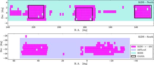
KiDS-450 survey footprint. Each pink box corresponds to a single KiDS pointing of 1 deg2. The turquoise region indicates the overlapping BOSS coverage and the blue region represents the 2dFLenS area. The black outlined rectangles are the GAMA spectroscopic fields that overlap with the KiDS-North field.

Figure 1.

KiDS-450 survey footprint. Each pink box corresponds to a single KiDS pointing of 1 deg². The turquoise region indicates the overlapping BOSS coverage and the blue region represents the 2dFLenS area. The black outlined rectangles are the GAMA spectroscopic fields that overlap with the KiDS-North field.

Open in new tab Download slide

The redshift distribution for KiDS galaxies was determined via four different approaches, which were shown to produce consistent results in a cosmic shear analysis (Hildebrandt et al. 2017). We adopt the preferred method of that analysis, the ‘weighted direct calibration’ (DIR) method, which exploits an overlap with deep spectroscopic fields. Following the work of Lima et al. (2008), the spectroscopic galaxies are re-weighted such that any incompleteness in their spectroscopic selection functions is removed. A sample of KiDS galaxies is selected using their associated z_B value, estimated from the four-band photometry as the peak of the redshift posterior output by the Bayesian photometric redshift bpz code (Benítez 2000). The true redshift distribution for the KiDS sample is determined by matching these to the re-weighted spectroscopic catalogue. The resulting redshift distribution is well calibrated in the range 0.1 < z_B ≤ 0.9.

KiDS has spectroscopic overlap with the Baryon Oscillation Spectroscopic Survey (BOSS) and the Galaxy And Mass Assembly (GAMA) survey in its northern field and the 2-degree Field Lensing Survey (2dFLenS) in the south. The footprints of the different data sets used in this analysis are shown in Fig. 1 and the effective overlapping areas are quoted in Table 1.

Table 1.

Open in new tab

For each spectroscopic survey used in the analysis, this table quotes the full area used for the clustering analysis, A_full, the overlapping effective area A_eff with the KiDS imaging, and the number of lenses in the overlap region of each sample that were used in the lensing analyses. Also quoted are the mean redshift of the spectroscopic sample and the RSD measurements of the β parameter, taken from Blake et al. (2016b) for 2dFLenS, Singh et al. (2018) for the BOSS samples, and Blake et al. (2013) for the analysis with GAMA.

Spec. sample	A_full (deg²)	A_eff (deg²)	N_lenses	\|$\overline{z}$\|	β
GAMA	180	144	33682	0.267	0.60 ± 0.09
LOWZ	8337	125	5656	0.309	0.41 ± 0.03
CMASS	9376	222	21341	0.548	0.34 ± 0.02
2dFLOZ	731	122	3014	0.300	0.49 ± 0.15
2dFHIZ	731	122	4662	0.560	0.26 ± 0.09

Spec. sample	A_full (deg²)	A_eff (deg²)	N_lenses	\|$\overline{z}$\|	β
GAMA	180	144	33682	0.267	0.60 ± 0.09
LOWZ	8337	125	5656	0.309	0.41 ± 0.03
CMASS	9376	222	21341	0.548	0.34 ± 0.02
2dFLOZ	731	122	3014	0.300	0.49 ± 0.15
2dFHIZ	731	122	4662	0.560	0.26 ± 0.09

Table 1.

Open in new tab

For each spectroscopic survey used in the analysis, this table quotes the full area used for the clustering analysis, A_full, the overlapping effective area A_eff with the KiDS imaging, and the number of lenses in the overlap region of each sample that were used in the lensing analyses. Also quoted are the mean redshift of the spectroscopic sample and the RSD measurements of the β parameter, taken from Blake et al. (2016b) for 2dFLenS, Singh et al. (2018) for the BOSS samples, and Blake et al. (2013) for the analysis with GAMA.

Spec. sample	A_full (deg²)	A_eff (deg²)	N_lenses	\|$\overline{z}$\|	β
GAMA	180	144	33682	0.267	0.60 ± 0.09
LOWZ	8337	125	5656	0.309	0.41 ± 0.03
CMASS	9376	222	21341	0.548	0.34 ± 0.02
2dFLOZ	731	122	3014	0.300	0.49 ± 0.15
2dFHIZ	731	122	4662	0.560	0.26 ± 0.09

Spec. sample	A_full (deg²)	A_eff (deg²)	N_lenses	\|$\overline{z}$\|	β
GAMA	180	144	33682	0.267	0.60 ± 0.09
LOWZ	8337	125	5656	0.309	0.41 ± 0.03
CMASS	9376	222	21341	0.548	0.34 ± 0.02
2dFLOZ	731	122	3014	0.300	0.49 ± 0.15
2dFHIZ	731	122	4662	0.560	0.26 ± 0.09

3.2 Spectroscopic overlap surveys

BOSS is a spectroscopic follow-up of the SDSS imaging survey, which used the Sloan Telescope to obtain redshifts for over a million galaxies spanning ∼ 10 000 deg². BOSS used colour and magnitude cuts to select two classes of galaxies: the ‘LOWZ’ sample, which contains Luminous Red Galaxies (LRGs) at z_l < 0.43, and the ‘CMASS’ sample, which is designed to be approximately stellar mass limited for z_l > 0.43. We used the data catalogues provided by the SDSS 12th Data Release (DR12); full details of these catalogues are given by Alam et al. (2015a). Following standard practice, we select objects from the LOWZ and CMASS data sets with 0.15 < z_l < 0.43 and 0.43 < z_l < 0.7, respectively, to create homogeneous galaxy samples. In order to correct for the effects of redshift failures, fibre collisions, and other known systematics affecting the angular completeness, we use the completeness weights assigned to the BOSS galaxies (Ross et al. 2017), denoted as w_l. The RSD parameters, β for LOWZ and CMASS are quoted in Table 1 and were drawn from Singh et al. (2018), who follow the method described in Alam et al. (2015b). This analysis used the monopole and quadrupole moments of the galaxy autocorrelation function, obtained by projecting the redshift-space correlation function on the Legendre basis. These multipole moments were fitted in each case applying a perturbation theory model, using scales larger than 28h⁻¹Mpc and fixing the Alcock–Paczynski parameters. This fitting range excludes the small scales that are used in our clustering and lensing measurements and we therefore assume that the RSD parameters are relatively constant across linear scales. An improvement to future E_G measurements can come from better RSD modelling to the small scales.

2dFLenS is a spectroscopic survey conducted by the Anglo-Australian Telescope with the AAOmega spectrograph, spanning an area of 731 deg² (Blake et al. 2016b). It is principally located in the KiDS regions, in order to expand the overlap area between galaxy redshift samples and gravitational lensing imaging surveys. The 2dFLenS spectroscopic data set contains two main target classes: ∼40 000 LRGs across a range of redshifts z_l < 0.9, selected by BOSS-inspired colour cuts (Dawson et al. 2013), as well as a magnitude-limited sample of ∼30 000 objects in the range 17 < r < 19.5, to assist with direct photometric calibration (Bilicki et al. 2017; Wolf et al. 2017). In our study, we analyse the 2dFLenS LRG sample, selecting redshift ranges 0.15 < z_l < 0.43 for ‘2dFLOZ’ and 0.43 < z_l < 0.7 for ‘2dFHIZ’, mirroring the selection of the BOSS sample. We refer the reader to Blake et al. (2016b) for a full description of the construction of the 2dFLenS selection function and random catalogues. The RSD parameter was determined by Blake et al. (2016b) from a fit to the multipole power spectra and was found to be β = 0.49 ± 0.15 and β = 0.26 ± 0.09 in the low- and high-redshift LRG samples, respectively. We present the 2dFLenS data release in Section 7.

GAMA is a spectroscopic survey carried out on the Anglo-Australian Telescope with the AAOmega spectrograph. We use the GAMA galaxies from three equatorial regions, G9, G12, and G15 from the third GAMA data release (Liske et al. 2015). These equatorial regions encompass roughly 180 deg², containing ∼180 000 galaxies with sufficient quality redshifts. The magnitude-limited sample is essentially complete down to a magnitude of r = 19.8. For our galaxy–galaxy lensing and clustering measurements, we use all GAMA galaxies in the three equatorial regions in the redshift range 0.15 < z_l < 0.51. As GAMA is essentially complete, the sample is equally weighted, such that w_l = 1 for all galaxies. We constructed random catalogues using the GAMA angular selection masks combined with an empirical smooth fit to the observed galaxy redshift distribution (Blake et al. 2013). We use the value for the RSD parameter from Blake et al. (2013) as β = 0.60 ± 0.09, which, we note encompasses a slightly different redshift range of 0.25 < z_l < 0.5, but still encompasses roughly 60 per cent of the galaxies in the sample. The use of this measurement is justified as β varies slowly with redshift, and therefore any systematic uncertainty introduced by this choice is smaller than the statistical error of the measurement. This analysis measured β similarly to the 2dFLenS case.

3.3 Mocks

We compute the full covariance between the different scales of the galaxy–galaxy lensing measurement using a large suite of N-body simulations, built from the Scinet Light Cone Simulations (SLICS; Harnois-Déraps & van Waerbeke 2015) and tailored for weak lensing surveys. These consist of 600 independent dark matter only simulations, in each of which 1536³ particles are evolved within a cube of |$505 h^{-1} \rm {Mpc}$| on a side and projected on 18 redshift mass planes between 0 < z < 3. Light-cones are propagated on these planes on 7745³ pixel grids and turned into shear maps via ray-tracing, with an opening angle of 100 deg². The cosmology is set to |$\rm {WMAP9 + BAO + SN}$| (Dunkley et al. 2009), that is Ω_m = 0.2905, Ω_Λ = 0.7095, Ω_b = 0.0473, h = 0.6898, n_s = 0.969, and σ₈ = 0.826. These mocks are fully described by Harnois-Déraps & van Waerbeke (2015) and a previous version with a smaller opening angle of 60 deg² was used in the KiDS analyses of Hildebrandt et al. (2017) and Joudaki et al. (2018).

Source galaxies are randomly inserted in the mocks, with a true redshift satisfying the KiDS DIR redshift distribution and a mock photometric redshift, z_B. The source number density is defined to reflect the effective number density of the KiDS data. The gravitational shears are an interpolation of the simulated shear maps at the galaxy positions, while the distribution of intrinsic ellipticity matches a Gaussian with a width of 0.29 per component, closely matching the measured KiDS intrinsic ellipticity dispersion (Hildebrandt et al. 2017; Amon et al. 2018).

To simulate a foreground galaxy sample, we populate the dark matter haloes extracted from the N-body simulations with galaxies, following a halo occupation distribution (HOD) approach that is tailored for each galaxy survey. The details of their construction and their ability to reproduce the clustering and lensing signals with the KiDS and spectroscopic foreground galaxy samples are described in Harnois-Deraps et al. (2018). Here, we summarize the strategy. Dark matter haloes are assigned a number of central and satellite galaxies based on their mass and on the HOD prescription. Centrals are placed at the halo centre and satellites are scattered around it following a spherically symmetric NFW profile, with the number of satellites scaling with the mass of the halo. On average, about 9 per cent of all mock CMASS and LOWZ galaxies are satellites, a fraction that closely matches that from the BOSS data. The satellite fraction in the GAMA mocks is closer to 15 per cent.

The CMASS and LOWZ HODs are inspired by the prescription of Alam et al. (2017) while the GAMA mocks follow the strategy of Smith et al. (2017). In all three cases, we adjust the value of some of the best-fitting parameters in order to enhance the agreement in clustering between mocks and data, while also closely matching the number density and the redshift distribution of the spectroscopic surveys. In contrast to the CMASS and LOWZ mocks, the GAMA mocks are constructed from a conditional luminosity function and galaxies are assigned an apparent magnitude such that we can reproduce the magnitude distribution of the GAMA data. For 2dFLenS, the LOWZ and CMASS mocks were subsampled to match the sparser 2dFLOZ and 2dFHIZ samples.

4 MEASUREMENTS

4.1 Galaxy–galaxy annular surface density

We compute the projected correlation function, w_p and the associated galaxy–galaxy annular surface density, Υ_gg, using the three-dimensional positional information for each of the five spectroscopic lens samples. We measure these statistics using random catalogues that contain N_ran galaxies, roughly 40 times the size of the galaxy sample, N_gal, with the same angular and redshift selection. To account for this difference, we assign each random point a weight of N_gal/N_ran.

Adopting a fiducial flat ΛCDM WMAP cosmology (Komatsu et al. 2011) with Ω_m = 0.27, we estimate the 3D galaxy correlation function, ξ_gg(R, Π), as a function of comoving projected separation, R, and line-of-sight separation, Π, using the estimator proposed by Landy & Szalay (1993),

\begin{eqnarray*} \xi _{\rm gg}(R,\Pi)=\rm {\frac{dd-2dr+rr}{rr}}\, , \end{eqnarray*}

(25)

where |$\rm {dd, rr}$|⁠, and |$\rm {dr}$| denote the weighted number of pairs with a separation (R, Π), where both objects are either in the galaxy catalogue, the random catalogue or one in each of the catalogues, respectively.

In order to obtain the projected correlation function, we combine the line-of-sight information by summing over 10 logarithmically spaced bins in Π from Π = 0.1 to |$\Pi =100 \, h^{-1}$|Mpc,

\begin{eqnarray*} w_{\rm p}(R)=2 \sum _i \xi _{\rm gg}(R, \Pi _i) \Delta \Pi _i \, . \end{eqnarray*}

(26)

We use 17 logarithmic bins in R from R = 0.05 to |$R=100 \, h^{-1}$|Mpc. The upper bound |$\Pi _{\rm max}=100 \, h^{-1}$|Mpc can potentially create a systematic error as R approaches Π_max due to any lost signal in the range |$\Pi >100 \, h^{-1}$|Mpc, however the signal is negligible on these scales . The error in w_p(R) is determined via a jackknife analysis, dividing the galaxy survey into 50 regions, ensuring a consistent shape and number of galaxies in each region. As such, the jackknife box size depends on the size of the survey at roughly 1 deg² for GAMA and a few square degrees for the other lens samples.

We convert this measurement to a galaxy–galaxy annular differential surface density (ADSD), Υ_gg, following equation (16), where we define R₀ = 2.0h⁻¹Mpc. A range of values of R₀ were tested between 1.0 and |$3.0 \, h^{-1}$|Mpc and it was found that this choice affected only the first R > R₀ data point, but had no significant effect on the value of the E_G measurement over all other scales. As such, scales below R = 5.0h⁻¹Mpc are not included. This choice removes regions where non-linear bias effects may enter, as well as account for any bias introduced by this choice of R₀. We determine w_p(R₀) via a power-law fit to the data in the range R₀/3 < R < 3R₀ and perform a linear interpolation to the measured w_p(R) in order to compute the integral in the first term. Any error in the interpolation for w_p(R₀) is ignored in the propagation of the jackknife error in w_p(R) to Υ_gg, as this contribution is only significant when R ≈ R₀.

The right-hand panel of Fig. 2 shows the measurements of |$\Upsilon _{\rm gg}(R,R_0=2.0 h^{-1} \rm {Mpc})$| for each of the lens samples.

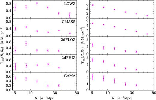
$The galaxy–matter (left) and galaxy–galaxy (right) annular differential surface density measurements as a function of comoving scale, $\Upsilon _{\rm gm}(R,R_0=2.0\, h^{-1} \rm {Mpc})$ and $\Upsilon _{\rm gg}(R,R_0=2.0 h^{-1} \rm {Mpc})$, respectively, with LOWZ, CMASS, 2dFLOZ, 2dFHIZ, and GAMA lens galaxy samples, from top to bottom. Scales below $R=5.0 \, h^{-1} \rm {Mpc}$ are not included in the analysis in order to remove regions where non-linear bias effects may enter, as well as to account for any bias introduced in the choice of R0. For Υgm, errors are from simulations, while the error on Υgg is determined from the propagation of a jackknife analysis.$

Figure 2.

The galaxy–matter (left) and galaxy–galaxy (right) annular differential surface density measurements as a function of comoving scale, |$\Upsilon _{\rm gm}(R,R_0=2.0\, h^{-1} \rm {Mpc})$| and |$\Upsilon _{\rm gg}(R,R_0=2.0 h^{-1} \rm {Mpc})$|⁠, respectively, with LOWZ, CMASS, 2dFLOZ, 2dFHIZ, and GAMA lens galaxy samples, from top to bottom. Scales below |$R=5.0 \, h^{-1} \rm {Mpc}$| are not included in the analysis in order to remove regions where non-linear bias effects may enter, as well as to account for any bias introduced in the choice of R₀. For Υ_gm, errors are from simulations, while the error on Υ_gg is determined from the propagation of a jackknife analysis.

Open in new tab Download slide

4.2 Galaxy–matter annular surface density

The galaxy–galaxy lensing estimator is defined as a function of angular separation in terms of the lensfit weight of the sources, w_s, the spectroscopic weight of the lenses, w_l, and the tangential ellipticity of the source relative to the lens, ε_t, as

\begin{eqnarray*} \gamma _{\rm t}(\theta)=\frac{\sum ^{\rm N_{pairs}}_{jk} w_{\rm s}^j w_{\rm l}^k \epsilon _t^{jk}}{\sum ^{\rm N_{pairs}}_{jk} w_{\rm s}^j w_{\rm l}^k} \, . \end{eqnarray*}

(27)

This statistic is measured with a selection function such that only source–lens galaxy pairs within a separation in the interval [θ, θ + Δθ] are probed. For this measurement, we employ the treecorr software of Jarvis, Bernstein & Jain (2004), but we have performed consistency checks using the athena software of Kilbinger, Bonnett & Coupon (2014).

Lens galaxies were selected by their spectroscopic redshift, z_l, into N_z redshift ‘slices’ of width Δz_l = 0.01 between 0.15 < z_l < 0.43 for LOWZ and 2dFLOZ, 0.15 < z_l < 0.51 for GAMA and 0.43 < z_l < 0.7 for CMASS and 2dFHIZ. For each slice of the lens catalogue, the tangential shear was measured in 17 logarithmic angular bins where the minimum and maximum angles were determined by the redshift of the lens slice as θ = R/χ(z_l) in order for all slice measurements to satisfy minimum and maximum comoving projected radii from the lens of R = 0.05 and |$R=100 \, h^{-1}$|Mpc. For each slice measurement, the source sample is limited to those behind each lens slice, in order to minimize the dilution of the lensing signal due to sources associated with the lens. The selection is made using the z_B photometric redshift estimate as z_B > z_l + 0.1, which was deemed most optimal in appendix D of Amon et al. (2018). The redshift distribution for each source subsample, N(z_s), is computed with the DIR method for each spectroscopic slice.

The inverse comoving critical surface mass density is calculated per source-lens slice following equation 6 and 8 as,

\begin{eqnarray*} \overline{\Sigma }_{\rm c, com}^{-1}[z_{\rm l},{N}(z_{\rm s})] = \frac{4\pi G (1+z_{\rm l}) \chi (z_{\rm l})}{c^2} \int ^{\infty }_{z_{\rm l}} \mathrm{ d}z_{\rm s} \, {N}(z_{\rm s}) \Big [1- \frac{\chi (z_{\rm l})}{\chi (z_{\rm s})}\Big ], \end{eqnarray*}

(28)

where |$\overline{\Sigma }_{\rm c, com}^{-1}[z_{\rm l},{N}(z_{\rm s})]$| is the inverse critical surface mass density at z_l, averaged over the entire source redshift distribution, N(z_s), normalized such that ∫N(z_s)dz_s = 1. χ(z_l) and χ(z_s) are the comoving distances to the lens and source galaxies, respectively. Again, we adopt a fiducial flat ΛCDM WMAP cosmology with Ω_m = 0.27. Our motivation for this choice is to ensure an unbiased measurement by choosing a cosmology with a value for the matter density which lies between the values favoured by KiDS and Planck. This also ensures consistency with the fiducial cosmological model adopted for the RSD analyses of the BOSS and GAMA analysis, which would be subject to Alcock–Paczynski distortion in different models (Alcock & Paczynski 1979). Adopting the different value of Ω_m preferred by the Planck and KiDS analyses would not produce a significant change in our measurements compared to their statistical errors.

The estimator for the excess surface mass density is defined as a function of the projected radius and the spectroscopic redshift of the lens as a combination of the inverse critical surface mass density and the tangential shear,

\begin{eqnarray*} \Delta \Sigma _{\rm com}(R,z_{\rm l})=\frac{\gamma _{\rm t}[\theta =R/\chi (z_{\rm l})]}{\overline{\Sigma _{\rm c,com}^{-1}}[z_{\rm l},N(z_{\rm s})]} \, . \end{eqnarray*}

(29)

We calculate the tangential shear and the differential surface mass density, ΔΣ(R), for each of the N_z lens slices and stack these signals to obtain an average differential surface mass density, weighted by the number of pairs in each slice as

\begin{eqnarray*} \overline{\Delta \Sigma }_{\rm com}(R)=\frac{\sum ^{N_{\rm z}}_i [\gamma _{\rm t}(R/\chi _{\rm l})/\overline{\Sigma _{\rm c,com}^{-1}}]^i n_{\rm {pairs}}^i \ K^i}{\sum ^{N_{\rm z}}_i n_{\rm {pairs}}^i} \, , \end{eqnarray*}

(30)

where we include a shear calibration for each redshift slice Kⁱ, where

\begin{eqnarray*} K^i=\frac{\sum _{\rm s} w_{\rm s} (1+m_{\rm s})}{\sum _{\rm s} w_{\rm s}} \, , \end{eqnarray*}

(31)

and m_s is the multiplicative bias per source galaxy as derived in Fenech Conti et al. (2017).

While it is common to apply a ‘boost factor’ in order to account for source galaxies that are physically associated with the lenses that may bias the tangential shear measurement, we show in Amon et al. (2018) that this signal is negligible for our lens samples and redshift selections for scales beyond |$R=2.0 \, h^{-1}$|Mpc. As we only probe larger scales than this, we do not apply this correction. The excess surface mass density was also computed around random points in the areal overlap. This signal has an expectation value of zero in the absence of systematics. As demonstrated by Singh et al. (2016), it is important that a random signal, ΔΣ_rand(R), is subtracted from the measurement in order to account for any small but non-negligible coherent additive bias of the galaxy shapes and to decrease large-scale sampling variance. The random signals were found to be consistent with zero for each lens sample (Amon et al. 2018).

The error in the measurements of |$\overline{\Delta \Sigma }(R)$| combines in quadrature the uncertainty in the random signal and the full covariance determined from simulations, as described in Section 4.3. A bootstrap analysis of the redshift distribution in Hildebrandt et al. (2017) revealed that this uncertainty is negligible compared to the lensing error budget for our analysis, as was also found in Dvornik et al. (2017).

We convert the measurements of the excess surface mass density and its covariance into the galaxy–matter ADSD, Υ_gm, following equation (15), with R₀ = 2.0h⁻¹Mpc. Similarly to the case of Υ_gg, we determine ΔΣ(R₀) by a power-law fit to the data and ignore any error on this interpolation.

The left-hand panel of Fig. 2 shows the measurements of |$\Upsilon _{\rm gm}(R,R_0=2.0 h^{-1} \rm {Mpc})$| for the cross-correlation with each of the lens samples. The ranges plotted, that is 5 < R < 60h⁻¹ for LOWZ and CMASS and 5 < R < 40h⁻¹Mpc for 2dFLOZ, 2dFHIZ, and GAMA, represent the scales where the assumption of linear bias holds and where we trust the jackknife error analysis for the clustering measurements in the cases of 2dFLenS and BOSS. These are the scales used in the measurements and fits of E_G(R). We note that the shapes and amplitudes of the lensing profiles on the left-hand side of Fig. 2 differ reflecting that the lens galaxy samples vary in flux limits and redshift and for the case of comparison between BOSS and 2dFLenS, completeness.

4.3 Covariance for E_G

We measure the galaxy–galaxy lensing signal using the ensemble of N_sim = 600 N-body simulations of source and lens catalogues with the same pipeline applied to the data. We construct the covariance matrix from these measurements by scaling the resulting covariance by |$100\, \rm {deg}^2/\mathit{ A}_{\rm eff}$| for each region, where A_eff represents the effective overlap area of the surveys, as listed in Table 1 (Schneider et al. 2002). The covariance, C, between the measurements at transverse scales Rⁱ and R^j, is computed as

\begin{eqnarray*} \hat{C}^{i,j}&=&\hat{C}[\Upsilon _{\rm gm}(R^i),\Upsilon _{\rm gm}(R^j)]=\frac{1}{N_{\rm sim} -1}\nonumber\\ &&\times \Big [ \sum _{k=1}^{N_{\rm {sim}}} \big (\Upsilon ^k_{\rm gm}(R^{i}) - \overline{\Upsilon _{\rm gm}}(R^i) \big) \big (\Upsilon ^k_{\rm gm}(R^{j}) -\overline{\Upsilon _{\rm gm}}(R^j) \big) \Big ], \end{eqnarray*}

(32)

where |$\Upsilon _{\rm gm}^k(R^i)$| is measured for the kth mock catalogue and |$\overline{\Upsilon _{\rm gm}}(R^i)$| is the average over all mocks.

Under the assumption that the three measurements that we combine to estimate E_G are independent, we estimate the covariance matrix as a combination of the covariance of the galaxy–galaxy lensing measurement estimated from N-body simulations, the jackknife covariance for the clustering measurement and the error in the β parameter, which modifies all scales and therefore folds through as a scalar of amplitude σ_β multiplied by a unit matrix. Using the chain rule for ratios, we obtain

\begin{eqnarray*} \frac{\hat{C}(E_{\rm G})^{i,j}}{E_{\rm G}^iE_{\rm G}^j}=\frac{\hat{C}(\Upsilon _{\rm gm})^{i,j}}{\Upsilon _{\rm gm}^i\Upsilon _{\rm gm}^j} + \frac{\hat{C}(\Upsilon _{\rm gg})^{i,j}}{\Upsilon _{\rm gg}^i\Upsilon _{\rm gg}^j} + \Big (\frac{\sigma _{\beta }}{\beta } \Big)^2 \, . \end{eqnarray*}

(33)

In Appendix A, we show the covariance matrix for each of the additive components of equation(33) and thereby demonstrate that the error in the clustering measurement is subdominant compared to the galaxy–galaxy lensing measurement, justifying our use of a jackknife approach rather than mock analysis for this clustering component. For the cases of BOSS and 2dFLenS analyses, the lensing measurements use a small fraction of the total area used for the clustering measurement. This justifies our choice to neglect the cross-covariance between the two measurements and assume that the lensing, clustering, and RSD measurements are independent. In Appendix A, we discuss the case of GAMA and the appropriateness of these assumptions, given that the lensing area is not significantly smaller than the clustering area. The errors in the measurements of the RSD parameter, β, are drawn from the literature and quoted in Table 1.

The inverse of this covariance matrix is used in the model fitting of E_G(R). Whilst we consider our measurement of |$\hat{C}(E_{\rm G})$| from the simulations to be an unbiased estimator of the true covariance matrix |$\hat{C}$|⁠, it will have an associated measurement noise as it is constructed from a finite number of semi-independent realizations. As such, |$\hat{C}^{-1}$| is not an unbiased estimate of the true inverse covariance matrix. We correct for this bias due to its maximum-likelihood estimation (Hartlap, Simon & Schneider 2007) as |$C^{-1}=\alpha \ \hat{C}^{-1}$|⁠, where

\begin{eqnarray*} \alpha =\frac{N_{\rm sim} - N_{\rm bin} - 2}{N_{\rm sim}-1}\, , \end{eqnarray*}

(34)

and N_bin is the number of data bins used in the fit. This correction is valid under the condition that the number of simulations exceeds the number of data bins with N_bin/N_sim < 0.8. In this case of a large number of simulations, the correction by Hartlap et al. (2007) gives the same results as the more robust correction of Sellentin & Heavens (2016).

The correlation matrix for E_G is determined from the covariance as

\begin{eqnarray*} \zeta (E_{\rm G})^{i,j}=\frac{\hat{C}(E_{\rm G})^{ij}}{\sqrt{\hat{C}(E_{\rm G})^{ii}\hat{C}(E_{\rm G})^{jj}}} \, . \end{eqnarray*}

(35)

Fig. 3 illustrates the correlation matrices of the measurements with each of the five lens samples. The correlation between different physical scales is most significant for cross-correlations with GAMA and 2dFHIZ and is non-negligible for the high-redshift samples.

Figure 3.

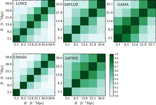
Correlation coefficients, ζ, defined by equation (35), of the covariance matrix of the E_G measurements, determined with each of the five lens samples. These are computed as a combination of the Υ_gm covariance determined from the scatter across the 600 simulation line of sights, the jackknife covariance of Υ_gg and the uncertainty on the RSD parameter, β.

Open in new tab Download slide

5 COSMOLOGICAL RESULTS

We combine the lensing and clustering measurements with the redshift-space distortion parameters following equation (17). We note that while our analysis includes the uncertainty related to each redshift-space distortion measurement, any potential remaining systematic errors on β could bias the E_G result. Fig. 4 shows our measurements of E_G(R) for the low-redshift lens samples (left) and the high-redshift lens samples (right). The black-line represents the GR prediction, determined with the KiDS+2dFLenS+BOSS cosmology measured by Joudaki et al. (2018), that is, with a matter density today of Ω_m(z = 0) = 0.243 ± 0.038. The coloured lines denote the best-fitting scale-independent model, as determined by the minimum chi-squared using the covariance defined in equation (32).

Figure 4.

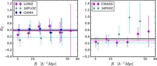
The E_G statistic, E_G(R), computed using KiDS-450 data combined with low-redshift spectroscopic lenses from GAMA (blue) in the range 0.15 < z_l < 0.51 and from 2dFLOZ (turquoise) and LOWZ (pink) in the range 0.15 < z_l < 0.43 in the left-hand panel and high-redshift lenses spanning 0.43 < z_l < 0.7 from CMASS (pink) and 2dFHIZ (turquoise) in the right-hand panel. Data points are offset on the R-axis for clarity. The solid black line denotes the GR prediction for a KiDS+2dFLenS+BOSS cosmology with Ω_m = 0.243 ± 0.038. The coloured lines denote the best-fitting scale-independent models to the measurements.

Open in new tab Download slide

The mean and 1σ error in the scale-independent best fit to the measurements, as shown in Fig. 4, are quoted for each lens sample in Table 2. The |$\chi ^2_{\rm min}$| for each of the analyses are quoted in the table. We note that the |$\chi ^2_{\rm min}$| for the analysis with GAMA is slightly lower than expected for four degrees of freedom. In Appendix A, we investigate the effect of the covariance on these fits for each of the lens samples. We argue that for the analysis with GAMA, the clustering error is overestimated due to the size of the jackknife region and causes an overestimation of the uncertainty of E_G, but is unlikely to bias the fit.

Table 2.

Open in new tab

The scale-independent fit to the E_G(R) measurements and the 1σ error on the parameter in the fit, along with the minimum χ² value and number of degrees of freedom (d.o.f.), for the analyses using each of the spectroscopic samples.

Spec. sample	E_G	\|$\chi ^2_{\rm min}$\|	d.o.f.
LOWZ	0.37 ± 0.12	2.8	5
2dFLOZ	0.18 ± 0.11	2.1	4
CMASS	0.28 ± 0.08	3.2	5
2dFHIZ	0.21 ± 0.12	3.4	4
GAMA	0.43 ± 0.13	0.8	4

Spec. sample	E_G	\|$\chi ^2_{\rm min}$\|	d.o.f.
LOWZ	0.37 ± 0.12	2.8	5
2dFLOZ	0.18 ± 0.11	2.1	4
CMASS	0.28 ± 0.08	3.2	5
2dFHIZ	0.21 ± 0.12	3.4	4
GAMA	0.43 ± 0.13	0.8	4

Table 2.

Open in new tab

The scale-independent fit to the E_G(R) measurements and the 1σ error on the parameter in the fit, along with the minimum χ² value and number of degrees of freedom (d.o.f.), for the analyses using each of the spectroscopic samples.

Spec. sample	E_G	\|$\chi ^2_{\rm min}$\|	d.o.f.
LOWZ	0.37 ± 0.12	2.8	5
2dFLOZ	0.18 ± 0.11	2.1	4
CMASS	0.28 ± 0.08	3.2	5
2dFHIZ	0.21 ± 0.12	3.4	4
GAMA	0.43 ± 0.13	0.8	4

Spec. sample	E_G	\|$\chi ^2_{\rm min}$\|	d.o.f.
LOWZ	0.37 ± 0.12	2.8	5
2dFLOZ	0.18 ± 0.11	2.1	4
CMASS	0.28 ± 0.08	3.2	5
2dFHIZ	0.21 ± 0.12	3.4	4
GAMA	0.43 ± 0.13	0.8	4

In Fig. 5 we plot the fits to our measurements as a function of the mean redshift of the spectroscopic sample in pink. BOSS and 2dFLenS are in different parts of the sky and therefore give independent measurements, which we find to be consistent with each other at roughly 1.5σ. As such, we combine the measurements at the same redshift using inverse-variance weighting and find |$E_{\rm G}(\overline{z}=0.305)=0.27 \pm 0.08$| for the combination of LOWZ+2dFLOZ and |$E_{\rm G}(\overline{z}=0.554)=0.26 \pm 0.07$| for the combination of CMASS+2dFHIZ. These combinations are denoted by larger pink data points. Alongside the results of this analysis, we plot existing measurements of E_G in black (Reyes et al. 2010; Blake et al. 2016a; Pullen et al. 2016; Alam et al. 2017; de la Torre et al. 2017). In light of the current tension between CMB temperature measurements from Planck and KiDS lensing data, we plot two GR predictions using both the preferred Planck cosmology (Planck Collaboration XIII 2016) and the KiDS+2dFLenS+BOSS cosmology (Joudaki et al. 2018). The Planck cosmology is drawn from Planck Collaboration XIII (2016), with Ω_m(z = 0) = 0.308 ± 0.009. The 68 per cent confidence regions are denoted by the shaded regions.

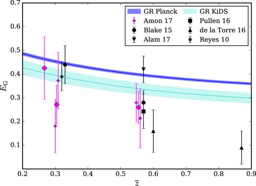
$The scale-independent fit to the EG(R) measurements shown in Fig. 4, now plotted as a function of the mean redshift of the spectroscopic lens sample, $E_{\rm G}(\overline{z})$. From left to right, the smaller pink data points represent the fits to the measurements computed using KiDS-450 combined with 2dFLOZ, LOWZ, CMASS and 2dFHIZ. The errorbars denote the 1σ uncertainty on the fit to the data. The larger pink data points represent the fit to the measurement with GAMA, as well as the combination of the independent fits from 2dFLOZ+LOWZ and 2dFHIZ+CMASS. The blue region denotes the 68 per cent confidence region of GR for a Planck (2016) cosmology while the turquoise region represents that for the KiDS+2dFLenS+BOSS cosmology.$

Figure 5.

The scale-independent fit to the E_G(R) measurements shown in Fig. 4, now plotted as a function of the mean redshift of the spectroscopic lens sample, |$E_{\rm G}(\overline{z})$|⁠. From left to right, the smaller pink data points represent the fits to the measurements computed using KiDS-450 combined with 2dFLOZ, LOWZ, CMASS and 2dFHIZ. The errorbars denote the 1σ uncertainty on the fit to the data. The larger pink data points represent the fit to the measurement with GAMA, as well as the combination of the independent fits from 2dFLOZ+LOWZ and 2dFHIZ+CMASS. The blue region denotes the 68 per cent confidence region of GR for a Planck (2016) cosmology while the turquoise region represents that for the KiDS+2dFLenS+BOSS cosmology.

Open in new tab Download slide

While the Reyes et al. (2010) result and the low-redshift Blake et al. (2016a) measurement of E_G are consistent with both the GR predictions, the high-redshift measurements show variation. Alam et al. (2017) found their high-redshift measurement of the E_G statistic to be consistent with both cosmologies. On the other hand, de la Torre et al. (2017), the high-redshift measurement from Blake et al. (2016a) and the CMB-lensing Pullen et al. (2016) measurement find values of the statistic that are more than 2σ low when compared to the Planck GR prediction. Notably, the highest redshift E_G measurements by de la Torre et al. (2017) are in tension with a KiDS+2dFLenS+BOSS GR prediction. The E_G statistic was motivated solely as a test of GR, but a choice of cosmology has to be made in computing this prediction. As Fig. 5 shows, this choice has a significant impact on conclusions. Interestingly, in general, our E_G measurements and previous measurements from the literature prefer lower values of the matter density parameter such as those constrained by KiDS+2dFLenS+BOSS.

In Fig. 6, we investigate our assumption of scale-independent bias. We show the prediction for E_G(R) in GR and with a KiDS cosmology, assuming a scale-dependent galaxy bias model using CMASS HOD parameters from More et al. (2015). Alongside, we plot the measurement with CMASS galaxies. The effect of including this scale-dependence is shown to be minimal in comparison with the errors on our measurements, which provides support for our assumption of linear bias on the projected scales in question. We do however caution that the bias model is fit to a marginally fainter galaxy population than the 2dFLenS LRG samples, and this prediction therefore only serves to illustrate the expected low-level impact of scale-dependent bias on our analysis. As GAMA contains less bright galaxies than CMASS, we assume that the effect of scale-dependent bias is smaller for this case. The value of E_G in GR with scale-dependent bias deviates from the scale-independent prediction by at most 10 per cent over the scales in which we are interested.

Figure 6.

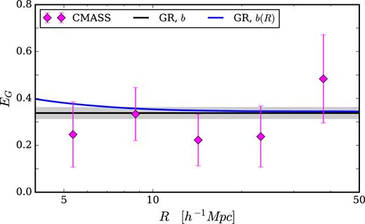
The effect of a scale-dependent galaxy bias on the predictions of the E_G statistic. We show E_G(R), computed with CMASS spectroscopic lenses (pink) plotted with the GR prediction for a KiDS+2dFLenS+BOSS cosmology with the fiducial scale-independent bias model, b, (black) and a scale-dependent bias model, b(R) (blue).

Open in new tab Download slide

Fig. 7 compares our three measurements to predictions of E_G(z) with modifications to GR in the phenomenological {μ₀, Σ₀} parametrization described in Section 2.6, with a Planck cosmology. We show variations to either μ₀ or Σ₀ and find that E_G is more sensitive to the latter.

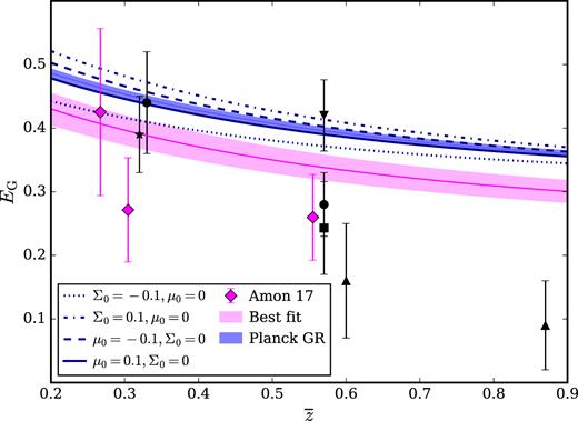
$Fits to the measurements of the EG statistic, $E_{\rm G}(\overline{z})$ measured with KiDS combined with GAMA, LOWZ+2dFLOZ and CMASS+2dFHIZ data compared to the theoretical predictions of the statistic with different gravity models for the Planck (2016) cosmology. The blue shaded region represents the prediction from GR, while the lines denote the theoretical predictions for modifications to gravity in a (Σ0, μ0) parametrization with different departures from (0,0). The pink shaded region reflects the best-fitting model for our EG measurements combined with that from Reyes et al. (2010), the low-redshift Blake et al. (2016a) and Alam et al. (2017).$

Figure 7.

Fits to the measurements of the E_G statistic, |$E_{\rm G}(\overline{z})$| measured with KiDS combined with GAMA, LOWZ+2dFLOZ and CMASS+2dFHIZ data compared to the theoretical predictions of the statistic with different gravity models for the Planck (2016) cosmology. The blue shaded region represents the prediction from GR, while the lines denote the theoretical predictions for modifications to gravity in a (Σ₀, μ₀) parametrization with different departures from (0,0). The pink shaded region reflects the best-fitting model for our E_G measurements combined with that from Reyes et al. (2010), the low-redshift Blake et al. (2016a) and Alam et al. (2017).

Open in new tab Download slide

6 SUMMARY AND OUTLOOK

We have performed a new measurement of the E_G statistic. This was achieved by using measurements of redshift-space distortions in 2dFLenS, GAMA, and BOSS galaxy samples and combining them with measurements of their galaxy–galaxy lensing signal, made using the first 450 deg² of the Kilo-Degree Survey. Our results are consistent with the prediction from GR for a perturbed FRW metric, in a ΛCDM Universe with a KiDS+2dFLenS+BOSS cosmology, given by Joudaki et al. (2018).

In particular, we determine E_G(z = 0.267) = 0.43 ± 0.13 using GAMA and averaging over scales 5 < R < 40h⁻¹Mpc, E_G(z = 0.305) = 0.27 ± 0.08 using a combination of LOWZ and 2dFLOZ and averaging over scales 5 < R < 60h⁻¹Mpc and E_G(z = 0.554) = 0.26 ± 0.07 using a combination of CMASS and 2dFHIZ over scales 5 < R < 60h⁻¹Mpc. To obtain these constraints, we fit a constant E_G model and incorporate the covariance matrix determined by a combination of the lensing covariance measured using a suite of N-body simulations, the clustering covariance determined from a jackknife analysis and the uncertainty on the RSD parameter, while neglecting them between the clustering and lensing measurements. In order to down-weight small scales where systematic corrections become significant and baryonic physics might have an effect, we suppress small-scale information from R < R₀ = 2.0h⁻¹Mpc using annular statistics for the projected clustering and differential surface mass density and find that above R = 5.0h⁻¹Mpc, our results are insensitive to the choice of R₀, consistent with previous analyses.

We show that while E_G is traditionally regarded a test of GR gravity, the robustness of this test is hindered by the uncertainty in the background cosmology, as illustrated by the current tensions between cosmological parameters defined by CMB temperature measurements from Planck and state of the art lensing data. While previous measurements of E_G (Reyes et al. 2010; Blake et al. 2016a; Pullen et al. 2016; de la Torre et al. 2017) have reported low measurements when compared to a GR prediction with a Planck cosmology (Planck Collaboration XIII 2016), similar to our findings, these apparent deviations are mostly resolved by a lower Ω_m cosmology. Using our measurements combined with literature measurements from Reyes et al. (2010), Blake et al. (2016a), and Alam et al. (2017), we find that the best-fitting model for E_G uses a cosmology with a matter density as Ω_m(z = 0) = 0.25 ± 0.03 with a |$\chi ^2_{\rm min}=6.3$| for five degrees of freedom. We present calculations of E_G in a two-parameter modified gravity scenario and show that 10 per cent changes in the metric potential amplitudes produce smaller differences in the predicted E_G than changing Ω_m between the values favoured by Planck and KiDS.

With Hyper Supreme-Cam (Aihara et al. 2018), as well as the advent of next-generation surveys like LSST,²Euclid,³WFIRST,⁴ 4MOST⁵ and DESI⁶ surveys, these cross-correlations and joint analyses will become increasingly important in testing our theories of gravity (Rhodes et al. 2013). However, we caution that measurements of the E_G statistic cannot be conducted as consistency checks of GR until the tension in cosmological parameters is resolved.

7 2dFLenS DATA RELEASE

Simultaneously with this paper, full data catalogues from 2dFLenS (a subset of which are used in our current analysis) will be released via the website http://2dflens.swin.edu.au. The construction of these catalogues is fully described by Blake et al. (2016b), and we briefly summarize the contents of the data release in this section.

The final 2dFLenS redshift catalogue contains 70 079 good-quality spectroscopic redshifts obtained by 2dFLenS across all target types. These include 40 531 LRGs spanning redshift range z < 0.9, 28 269 redshifts that form a magnitude-limited nearly complete galaxy subsample in the r-band magnitude range 17 < r < 19.5, and a number of other target classes including a point-source photometric-redshift training set, compact early-type galaxies, brightest cluster galaxies, and strong lenses.
The selection function of the LRG subsamples has been determined, as described by Blake et al. (2016b). The data release contains LRG data and random catalogues for low-redshift (0.15 < z < 0.43) and high-redshift (0.43 < z < 0.7) LRGs in the KiDS-South and KiDS-North regions, after merging the different LRG target populations.
Mock data and random catalogues for 2dFLenS LRGs were constructed by applying an HOD to an N-body simulation, as described by Blake et al. (2016b). The data release contains 65 mocks subsampled with the 2dFLenS selection function; the mock random catalogues slightly differ from the data random catalogues owing to approximations in mock generation (that are unimportant for cosmological applications).

ACKNOWLEDGEMENTS

We thank the anonymous referee for careful and thorough comments, Shadab Alam for his advice and for kindly sharing measurements of the RSD parameter from BOSS DR12, and Arun Kannawadi Jayaraman and Vasiliy Demchenko for useful comments. Furthermore, we thank the referee for careful and thorough comments. AA, CH, MA, and SJ acknowledge support from the European Research Council under grant numbers 647112 (CH and MA) and 693024 (SJ). CB acknowledges the support of the Australian Research Council through the award of a Future Fellowship. DL acknowledges support from the McWilliams Center for Cosmology, Department of Physics, Carnegie Mellon University. HHi acknowledges support from an Emmy Noether grant (No. Hi 1495/2-1) of the Deutsche Forschungsgemeinschaft. HHo acknowledges support from Vici grant 639.043.512, financed by the Netherlands Organisation for Scientific Research (NWO). BJ acknowledges support by an STFC Ernest Rutherford Fellowship, grant reference ST/J004421/1. JHD acknowledges support from the EuropeansCommission under a Marie-Sklodwoska-Curie European Fellowship (EU project 656869). SJ also acknowledges support from the Beecroft Trust. DP acknowledges the support of the Australian Research Council through the award of a Future Fellowship. MB is supported by the Netherlands Organisation for Scientific Research, NWO, through grant number 614.001.451.

This work is based on data products from observations made with ESO Telescopes at the La Silla Paranal Observatory under programme IDs 177.A-3016, 177.A-3017, and 177.A-3018, and on data products produced by Target/OmegaCEN, INAF-OACN, INAF-OAPD and the KiDS production team, on behalf of the KiDS consortium.

2dFLenS is based on data acquired through the Australian Astronomical Observatory, under programme A/2014B/008. It would not have been possible without the dedicated work of the staff of the AAO in the development and support of the 2dF-AAOmega system, and the running of the AAT.

We thank the GAMA consortium for providing access to their third data release. GAMA is a joint European-Australasian project based around a spectroscopic campaign using the Anglo-Australian Telescope. The GAMA input catalogue is based on data taken from the Sloan Digital Sky Survey and the UKIRT Infrared Deep Sky Survey. Complementary imaging of the GAMA regions is being obtained by a number of independent survey programmes including GALEX MIS, VST KiDS, VISTA VIKING, WISE, Herschel-ATLAS, GMRT, and ASKAP providing UV to radio coverage. GAMA is funded by the STFC (UK), the ARC (Australia), the AAO, and the participating institutions. The GAMA website is http://www.gama-survey.org/.

Computations for the N-body simulations were performed in part on the Orcinus supercomputer at the WestGrid HPC consortium (www.westgrid.ca), in part on the GPC supercomputer at the SciNet HPC Consortium. SciNet is funded by: the Canada Foundation for Innovation under the auspices of Compute Canada; the Government of Ontario; Ontario Research Fund – Research Excellence; and the University of Toronto.

Author contributions: All authors contributed to the development and writing of this paper. The authorship list is given in two groups: the lead authors (AA, CB, CH, DL), followed by an alphabetical group which includes those who have either made a significant contribution to the data products or to the scientific analysis.

Footnotes

1

We note that Σ_{c, com} is denoted as Σ_c in, for example, Mandelbaum et al. (2005), Leauthaud et al. (2017), Blake et al. (2016a), Miyatake et al. (2015), and Singh et al. (2016), whereas Σ_{c, phys} is denoted as Σ_c in, for example, van Uitert et al. (2011), Viola et al. (2015), and Prat et al. (2018).

2

http://www.lsst.org/

3

http://sci.esa.int/euclid/

4

http://wfirst.gsfc.nasa.gov/

5

https://www.4most.eu/cms/

6

http://desi.lbl.gov/

REFERENCES

Aihara

H.

et al. ,

2018

,

PASJ

,

70

,

S4

10.1093/pasj/psx066

Crossref

Alam

S.

et al. ,

2015a

,

ApJS

,

219

,

12

10.1088/0067-0049/219/1/12

Crossref

Search ADS

Alam

S.

,

Ho

S.

,

Vargas-Magaña

M.

,

Schneider

D. P.

,

2015b

,

MNRAS

,

453

,

1754

10.1093/mnras/stv1737

Crossref

Search ADS

Alam

S.

,

Miyatake

H.

,

More

S.

,

Ho

S.

,

Mandelbaum

R.

,

2017

,

MNRAS

,

465

,

4853

10.1093/mnras/stw3056

Crossref

Search ADS

Alcock

C.

,

Paczynski

B.

,

1979

,

Nature

,

281

,

358

10.1038/281358a0

Crossref

Search ADS

Amendola

L.

,

Kunz

M.

,

Saltas

I. D.

,

Sawicki

I.

,

2018

,

Phys. Rev. Lett.

,

120

,

131101

10.1103/PhysRevLett.120.131101

Crossref

Search ADS

PubMed

Amon

A.

et al. ,

2018

,

MNRAS

,

447

,

4285

10.1093/mnras/sty859

Crossref

Search ADS

Asgari

M.

,

Heymans

C.

,

Blake

C.

,

Harnois-Deraps

J.

,

Schneider

P.

,

Van Waerbeke

L.

,

2017

,

MNRAS

,

464

,

1676

10.1093/mnras/stw2436

Crossref

Search ADS

Baker

T.

,

Ferreira

P.

,

Skordis

C.

,

2014

,

Phys. Rev. D

,

89

,

024026

10.1103/PhysRevD.89.024026

Crossref

Search ADS

Baker

T.

,

Bellini

E.

,

Ferreira

P. G.

,

Lagos

M.

,

Noller

J.

,

Sawicki

I.

,

2017

,

Phys. Rev. Lett.

,

119

,

251301

Crossref

Search ADS

PubMed

Baldauf

T.

,

Smith

R. E.

,

Seljak

U.

,

Mandelbaum

R.

,

2010

,

Phys. Rev. D

,

81

,

063531

10.1103/PhysRevD.81.063531

Crossref

Search ADS

Bardeen

J. M.

,

1980

,

Phys. Rev. D

,

22

,

1882

10.1103/PhysRevD.22.1882

Crossref

Search ADS

Barreira

A.

,

Li

B.

,

Hellwing

W. A.

,

Baugh

C. M.

,

Pascoli

S.

,

2013

,

J. Cosmol. Astropart. Phys.

,

10

,

027

10.1088/1475-7516/2013/10/027

Crossref

Search ADS

Benítez

N.

,

2000

,

ApJ

,

536

,

571

10.1086/308947

Crossref

Search ADS

Bilicki

M.

et al. ,

2017

, preprint (arXiv:1709.04205)

Blake

C.

et al. ,

2013

,

MNRAS

,

436

,

3089

10.1093/mnras/stt1791

Crossref

Search ADS

Blake

C.

et al. ,

2016a

,

MNRAS

,

456

,

2806

10.1093/mnras/stv2875

Crossref

Search ADS

Blake

C.

et al. ,

2016b

,

MNRAS

,

462

,

4240

10.1093/mnras/stw1990

Crossref

Search ADS

Buddendiek

A.

et al. ,

2016

,

MNRAS

,

456

,

3886

10.1093/mnras/stv2925

Crossref

Search ADS

Cacciato

M.

,

Lahav

O.

,

van den Bosch

F. C.

,

Hoekstra

H.

,

Dekel

A.

,

2012

,

MNRAS

,

426

,

566

10.1111/j.1365-2966.2012.21762.x

Crossref

Search ADS

Cai

Y.-C.

,

Bernstein

G.

,

2012

,

MNRAS

,

422

,

1045

10.1111/j.1365-2966.2012.20676.x

Crossref

Search ADS

Copeland

E. J.

,

Sami

M.

,

Tsujikawa

S.

,

2006

,

Int. J. Mod. Phys. D

,

15

,

1753

10.1142/S021827180600942X

Crossref

Search ADS

Creminelli

P.

,

Vernizzi

F.

,

2017

,

Phys. Rev. Lett.

,

119

,

251302

10.1103/PhysRevLett.119.251302

Crossref

Search ADS

PubMed

Dawson

K. S.

et al. ,

2013

,

AJ

,

145

,

10

10.1088/0004-6256/145/1/10

Crossref

Search ADS

de Jong

J. T. A.

et al. ,

2017

,

A&A

,

604

,

A134

10.1051/0004-6361/201730747

Crossref

Search ADS

de la Torre

S.

et al. ,

2017

,

A&A

,

608

,

A44

10.1051/0004-6361/201630276

Crossref

Search ADS

Dekel

A.

,

Lahav

O.

,

1999

,

ApJ

,

520

,

24

10.1086/307428

Crossref

Search ADS

DES Collaboration

2017

, preprint (arXiv:1708.01530)

Driver

S. P.

et al. ,

2011

,

MNRAS

,

413

,

971

10.1111/j.1365-2966.2010.18188.x

Crossref

Search ADS

Dunkley

J.

et al. ,

2009

,

ApJS

,

180

,

306

10.1088/0067-0049/180/2/306

Crossref

Search ADS

Dvornik

A.

et al. ,

2017

,

MNRAS

,

468

,

3251

10.1093/mnras/stx705

Crossref

Search ADS

Edge

A.

,

Sutherland

W.

,

Kuijken

K.

,

Driver

S.

,

McMahon

R.

,

Eales

S.

,

Emerson

J. P.

,

2013

,

The Messenger

,

154

,

32

Ezquiaga

J. M.

,

Zumalacárregui

M.

,

2017

,

Phys. Rev. Lett.

,

119

,

251304

10.1103/PhysRevLett.119.251304

Crossref

Search ADS

PubMed

Fenech Conti

I.

,

Herbonnet

R.

,

Hoekstra

H.

,

Merten

J.

,

Miller

L.

,

Viola

M.

,

2017

,

MNRAS

,

467

,

1627

10.1093/mnras/stx200

Crossref

Ferreira

P. G.

,

Skordis

C.

,

2010

,

Phys. Rev. D

,

81

,

104020

10.1103/PhysRevD.81.104020

Crossref

Search ADS

Guzzo

L.

et al. ,

2008

,

Nature

,

451

,

541

Hamilton

A. J. S.

,

1993

,

ApJ

,

417

,

19

10.1086/173288

Crossref

Search ADS

Harnois-Déraps

J.

,

van Waerbeke

L.

,

2015

,

MNRAS

,

450

,

2857

10.1093/mnras/stv794

Crossref

Search ADS

Harnois-Deraps

J.

et al. ,

2018

, preprint (arXiv:1805.04511)

Hartlap

J.

,

Simon

P.

,

Schneider

P.

,

2007

,

A&A

,

464

,

399

10.1051/0004-6361:20066170

Crossref

Search ADS

Heymans

C.

et al. ,

2013

,

MNRAS

,

432

,

2433

10.1093/mnras/stt601

Crossref

Search ADS

Hildebrandt

H.

et al. ,

2017

,

MNRAS

,

465

,

1454

10.1093/mnras/stw2805

Crossref

Search ADS

Hoekstra

H.

,

Yee

H. K. C.

,

Gladders

M. D.

,

2004

,

ApJ

,

606

,

67

10.1086/382726

Crossref

Search ADS

Jain

B.

,

Zhang

P.

,

2008

,

Phys. Rev. D

,

78

,

063503

10.1103/PhysRevD.78.063503

Crossref

Search ADS

Jarvis

M.

,

Bernstein

G.

,

Jain

B.

,

2004

,

MNRAS

,

352

,

338

10.1111/j.1365-2966.2004.07926.x

Crossref

Search ADS

Joudaki

S.

,

Kaplinghat

M.

,

2012

,

Phys. Rev. D

,

86

,

023526

10.1103/PhysRevD.86.023526

Crossref

Search ADS

Joudaki

S.

et al. ,

2018

,

MNRAS

,

474

,

4894

10.1093/mnras/stx2820

Crossref

Search ADS

Kaiser

N.

,

1984

,

ApJ

,

284

,

L9

10.1086/184341

Crossref

Search ADS

Kaiser

N.

,

1987

,

MNRAS

,

227

,

1

10.1093/mnras/227.1.1

Crossref

Search ADS

Kilbinger

M.

,

Bonnett

C.

,

Coupon

J.

,

2014

,

Astrophysics Source Code Library, record ascl:1402.026

.

Google Scholar

Google Preview

OpenURL Placeholder Text

WorldCat

Komatsu

E.

et al. ,

2011

,

ApJS

,

192

,

18

10.1088/0067-0049/192/2/18

Crossref

Search ADS

Kuijken

K.

et al. ,

2015

,

MNRAS

,

454

,

3500

10.1093/mnras/stv2140

Crossref

Search ADS

Landy

S. D.

,

Szalay

A. S.

,

1993

,

ApJ

,

412

,

64

10.1086/172900

Crossref

Search ADS

Leauthaud

A.

et al. ,

2017

,

MNRAS

,

467

,

3024

10.1093/mnras/stx258

Crossref

Search ADS

Leonard

C. D.

,

Ferreira

P. G.

,

Heymans

C.

,

2015a

,

J. Cosmol. Astropart. Phys.

,

12

,

051

10.1088/1475-7516/2015/12/051

Crossref

Search ADS

Leonard

C. D.

,

Baker

T.

,

Ferreira

P. G.

,

2015b

,

Phys. Rev. D

,

91

,

083504

10.1103/PhysRevD.91.083504

Crossref

Search ADS

Li

B.

,

Barreira

A.

,

Baugh

C. M.

,

Hellwing

W. A.

,

Koyama

K.

,

Pascoli

S.

,

Zhao

G.-B.

,

2013

,

J. Cosmol. Astropart. Phys.

,

11

,

012

10.1088/1475-7516/2013/11/012

Crossref

Lima

M.

,

Cunha

C. E.

,

Oyaizu

H.

,

Frieman

J.

,

Lin

H.

,

Sheldon

E. S.

,

2008

,

MNRAS

,

390

,

118

10.1111/j.1365-2966.2008.13510.x

Crossref

Search ADS

Linder

E. V.

,

2005

,

Phys. Rev. D

,

72

,

043529

10.1103/PhysRevD.72.043529

Crossref

Search ADS

Liske

J.

et al. ,

2015

,

MNRAS

,

452

,

2087

10.1093/mnras/stv1436

Crossref

Search ADS

Lombriser

L.

,

Lima

N. A.

,

2017

,

Phys. Lett. B

,

765

,

382

10.1016/j.physletb.2016.12.048

Crossref

Search ADS

Lombriser

L.

,

Taylor

A.

,

2016

,

J. Cosmol. Astropart. Phys.

,

3

,

031

10.1088/1475-7516/2016/03/031

Crossref

Search ADS

Mandelbaum

R.

et al. ,

2005

,

MNRAS

,

361

,

1287

10.1111/j.1365-2966.2005.09282.x

Crossref

Search ADS

Mandelbaum

R.

,

Seljak

U.

,

Baldauf

T.

,

Smith

R. E.

,

2010

,

MNRAS

,

405

,

2078

10.1111/j.1365-2966.2010.16619.x

Crossref

Miller

L.

et al. ,

2013

,

MNRAS

,

429

,

2858

10.1093/mnras/sts454

Crossref

Search ADS

Miyatake

H.

et al. ,

2015

,

ApJ

,

806

,

1

10.1088/0004-637X/806/1/1

Crossref

Search ADS

More

S.

,

Miyatake

H.

,

Mandelbaum

R.

,

Takada

M.

,

Spergel

D. N.

,

Brownstein

J. R.

,

Schneider

D. P.

,

2015

,

ApJ

,

806

,

2

10.1088/0004-637X/806/1/2

Crossref

Search ADS

Noller

J.

,

von

Braun-Bates F.

,

Ferreira

P. G.

,

2014

,

Phys. Rev. D

,

89

,

023521

10.1103/PhysRevD.89.023521

Crossref

Search ADS

Planck Collaboration XIII

,

2016

,

A&A

,

594

,

A13

10.1051/0004-6361/201525830

Crossref

Search ADS

Pogosian

L.

,

Silvestri

A.

,

2008

,

Phys. Rev. D

,

77

,

023503

10.1103/PhysRevD.77.023503

Crossref

Search ADS

Prat

J.

et al. ,

2018

,

MNRAS

,

473

,

1667

10.1093/mnras/stx2430

Crossref

Search ADS

Pullen

A. R.

,

Alam

S.

,

He

S.

,

Ho

S.

,

2016

,

MNRAS

,

460

,

4098

10.1093/mnras/stw1249

Crossref

Search ADS

Reyes

R.

,

Mandelbaum

R.

,

Seljak

U.

,

Baldauf

T.

,

Gunn

J. E.

,

Lombriser

L.

,

Smith

R. E.

,

2010

,

Nature

,

464

,

256

Rhodes

J.

et al. ,

2013

, preprint (arXiv:1309.5388)

Ross

A. J.

et al. ,

2017

,

MNRAS

,

464

,

1168

10.1093/mnras/stw2372

Crossref

Search ADS

Sakstein

J.

,

Jain

B.

,

2017

,

Phys. Rev. Lett.

,

119

,

251303

10.1103/PhysRevLett.119.251303

Crossref

Search ADS

PubMed

Schmidt

F.

,

2009

,

Phys. Rev. D

,

80

,

043001

10.1103/PhysRevD.80.043001

Crossref

Search ADS

Schneider

P.

,

van Waerbeke

L.

,

Kilbinger

M.

,

Mellier

Y.

,

2002

,

A&A

,

396

,

1

10.1051/0004-6361:20021341

Crossref

Search ADS

Schneider

P.

,

Eifler

T.

,

Krause

E.

,

2010

,

A&A

,

520

,

A116

10.1051/0004-6361/201014235

Crossref

Search ADS

Sellentin

E.

,

Heavens

A. F.

,

2016

,

MNRAS

,

456

,

L132

10.1093/mnrasl/slv190

Crossref

Search ADS

Silvestri

A.

,

Pogosian

L.

,

Buniy

R. V.

,

2013

,

Phys. Rev. D

,

87

,

104015

10.1103/PhysRevD.87.104015

Crossref

Search ADS

Simpson

F.

et al. ,

2013

,

MNRAS

,

429

,

2249

10.1093/mnras/sts493

Crossref

Search ADS

Singh

S.

,

Mandelbaum

R.

,

Seljak

U.

,

Slosar

A.

,

Vazquez Gonzalez

J.

,

2016

, preprint (arXiv:1611.00752)

Singh

S.

,

Alam

S.

,

Mandelbaum

R.

,

Seljak

U.

,

Rodriguez-Torres

S.

,

Ho

S.

,

2018

, preprint (arXiv:1803.08915)

Smith

A.

,

Cole

S.

,

Baugh

C.

,

Zheng

Z.

,

Angulo

R.

,

Norberg

P.

,

Zehavi

I.

,

2017

,

MNRAS

,

470

,

4646

10.1093/mnras/stx1432

Crossref

Search ADS

Tereno

I.

,

Semboloni

E.

,

Schrabback

T.

,

2011

,

A&A

,

530

,

A68

10.1051/0004-6361/201016273

Crossref

Search ADS

Troxel

M. A.

et al. ,

2017

, preprint (arXiv:1708.01538)

van Uitert

E.

et al. ,

2018

,

MNRAS

,

476

,

4662

10.1093/mnras/sty551

Crossref

Search ADS

van Uitert

E.

,

Hoekstra

H.

,

Velander

M.

,

Gilbank

D. G.

,

Gladders

M. D.

,

Yee

H. K. C.

,

2011

,

A&A

,

534

,

A14

10.1051/0004-6361/201117308

Crossref

Search ADS

Viola

M.

et al. ,

2015

,

MNRAS

,

452

,

3529

10.1093/mnras/stv1447

Crossref

Search ADS

Wang

L.

,

Steinhardt

P. J.

,

1998

,

ApJ

,

508

,

483

10.1086/306436

Crossref

Search ADS

Weinberg

S.

,

1989

,

Revi. Mod. Phys.

,

61

,

1

10.1103/RevModPhys.61.1

Crossref

Search ADS

Weinberg

D. H.

,

Mortonson

M. J.

,

Eisenstein

D. J.

,

Hirata

C.

,

Riess

A. G.

,

Rozo

E.

,

2013

,

Phys. Rep.

,

530

,

87

10.1016/j.physrep.2013.05.001

Crossref

Search ADS

Wolf

C.

et al. ,

2017

,

MNRAS

,

466

,

1582

10.1093/mnras/stw3151

Crossref

Search ADS

Zhang

P.

,

Liguori

M.

,

Bean

R.

,

Dodelson

S.

,

2007

,

Phys. Rev. Lett.

,

99

,

141302

10.1103/PhysRevLett.99.141302

Crossref

Search ADS

PubMed

Zhao

G.

,

Bacon

D.

,

Maartens

R.

,

Santos

M.

,

Raccanelli

A.

,

2015

,

Advancing Astrophysics with the Square Kilometre Array (AASKA14)

, p.

165

Google Scholar

Google Preview

OpenURL Placeholder Text

WorldCat

Zhao

G.-B.

,

Pogosian

L.

,

Silvestri

A.

,

Zylberberg

J.

,

2009

,

Phys. Rev. D

,

79

,

083513

10.1103/PhysRevD.79.083513

Crossref

Search ADS

Zhao

G.-B.

,

Li

B.

,

Koyama

K.

,

2011

,

Phys. Rev. D

,

83

,

044007

10.1103/PhysRevD.83.044007

Crossref

Search ADS

APPENDIX A: E_G COVARIANCE

In Section 4.3, we compute the covariance for E_G following equation (33), where we incorporate a covariance for the lensing measurement estimated from a mock analysis, |$\hat{C}(\Upsilon _{\rm gm})$|⁠, a covariance of clustering measurement determined from a jackknife analysis, |$\hat{C}({\Upsilon _{\rm gg}})$| and the uncertainty on the RSD parameter, σ_β. In this Appendix, we investigate the contribution of each of these terms to the covariance for our final measurement. The E_G covariance in equation (33) can be written as the sum of a lensing term, D, a clustering term, W and a β term, B, as

\begin{eqnarray*} \hat{C}(E_{\rm G})=D+W+B\, , \end{eqnarray*}

(A1)

where, for example,

\begin{eqnarray*} D=(E_{\rm G}^iE_{\rm G}^j)\frac{\hat{C}(\Upsilon _{\rm gm})^{i,j}}{\Upsilon _{\rm gm}^i\Upsilon _{\rm gm}^j} \, , \end{eqnarray*}

(A2)

with the diagonal components denoted as D^d, where

\begin{eqnarray*} D^d=(E_{\rm G}^i)^2\frac{\hat{C}(\Upsilon _{\rm gm})^{i=j}}{(\Upsilon _{\rm gm}^i)^2} \, . \end{eqnarray*}

(A3)

Fig. A1 represents the different components of |$\hat{C}(E_{\rm G})$| for the analyses for each of the lens samples. In all cases it is evident that the left-hand panel, which shows the lensing covariance, D, defined in equation (A2), dominates compared to W the clustering jackknife covariance. This is expected as the lensing measurement is dominated by shape noise. This justifies the use of a jackknife covariance for the clustering measurement, rather than a full mock analysis. Furthermore, for all of the lens samples except for GAMA, the galaxy–galaxy lensing measurement uses asignificantly smaller area compared to that for the clustering and RSD measurement, rendering these measurements essentially independent. For the 2dFLenS analyses, especially 2dFHIZ, the contribution to the error budget from the RSD parameter is more significant. For the case of GAMA, with equal areas for all components of the E_G measurement, we show that while the lensing covariance is dominant, W and B are significant.

$The three different components of the EG(R) covariance in equations (A1) and (33) and their sum, for the analyses with each lens sample. From left to right, the panels show D, W, B, and $\hat{C}(E_{\rm G})$ with a consistent colour scale.$

Figure A1.

The three different components of the E_G(R) covariance in equations (A1) and (33) and their sum, for the analyses with each lens sample. From left to right, the panels show D, W, B, and |$\hat{C}(E_{\rm G})$| with a consistent colour scale.

Open in new tab Download slide

To further investigate the covariance, we compare the effects of the different components of the covariance on the best-fitting value and 1σ uncertainty in the fit for the E_G(R) measurement, as well as the associated |$\chi ^2_{\rm min}$| for the fit. The upper panels of Fig. A2 show the best scale-independent fits to the E_G(R) measurements for each of the lens samples and how they vary as the complexity of the E_G covariance is increased. That is, we consider using the diagonal of the lensing covariance computed from the mock analysis, D^d compared to the full covariance, D and follow the same convention adding in the clustering and RSD components. The lower panels show the associated |$\chi ^2_{\rm min}$| values for these fits.

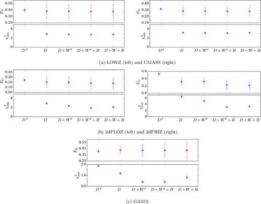
$The best-fitting value and 1σ uncertainty in the fit for the EG(R) measurements (upper panels) and the associated $\chi ^2_{\rm min}$ for the fit (lower panels) for the analyses with LOWZ, CMASS, 2dFLOZ, 2dFHIZ, and GAMA. From left to right along the horizontal axis, different components we added to the EG covariance (given in equation A1) in succession. For example, the first two data points compare the effect of using only the diagonal of the lensing covariance obtained from the mock analysis, Dd, with the full covariance D.$

Figure A2.

The best-fitting value and 1σ uncertainty in the fit for the E_G(R) measurements (upper panels) and the associated |$\chi ^2_{\rm min}$| for the fit (lower panels) for the analyses with LOWZ, CMASS, 2dFLOZ, 2dFHIZ, and GAMA. From left to right along the horizontal axis, different components we added to the E_G covariance (given in equation A1) in succession. For example, the first two data points compare the effect of using only the diagonal of the lensing covariance obtained from the mock analysis, D^d, with the full covariance D.

Open in new tab Download slide

In all cases, the most significant change in the best-fitting E_G, the associated uncertainty and the |$\chi ^2_{\rm min}$| was between D^d and D, emphasizing the importance of the off-diagonals in the lensing covariance. For CMASS, as is the case for LOWZ, the best-fitting E_G and the |$\chi ^2_{\rm min}$| are stable to the inclusion of the clustering and beta uncertainties, though the uncertainty on the fits increase.

For the cases of 2dFHIZ and 2dFLOZ shown in the middle panel of Fig. A2, the penultimate data point shows that the effect of including the uncertainty on the RSD parameter is to lower the best-fitting E_G. As revealed in Fig. A1, as the relative uncertainty of the RSD parameter is large for these two lens samples, the covariance between the large scales of the E_G measurement is amplified and therefore down-weighted. Therefore, the best fits to the data are slightly lower than expected when performing a ‘chi-by-eye’ analysisof Fig. 4.

For GAMA, we again show that the clustering covariance and the beta uncertainty contribute significantly to the final covariance for E_G. While the best fit does not change with increasing complexity, the |$\chi ^2_{\rm min}$| values do. The spuriously low |$\chi ^2_{\rm min}$| for the fits that include either W^d or W suggests that the clustering measurements are overestimated due to the size of the jackknife samples and this causes an overestimation of the uncertainty on our final measurement. Furthermore, the difference between the |$\chi ^2_{\rm min}$| for W^d and W suggest that the jackknife analysis for the clustering overestimates the uncertainty due to the limited jackknife box size.

We note that we have not accounted for any covariance between the clustering and RSD measurement. This effect would be more significant for 2dFLenS and GAMA as in these cases, the uncertainty on the lensing measurement is less dominant. However, both the uncertainty on the RSD measurements and the clustering measurements are shown in Fig. A2 to have at most, a 10 per cent shift on the value of E_G, compared to the uncertainty on the measurement, which is roughly 50 per cent. As such, we assume that any covariance between the RSD and clustering measurements will contribute less and can be safely ignored, given the precision of this analysis.

This article is published and distributed under the terms of the Oxford University Press, Standard Journals Publication Model (https://dbpia.nl.go.kr/journals/pages/about_us/legal/notices)

Download all slides

Month:	Total Views:
June 2018	5
July 2018	18
August 2018	33
September 2018	25
October 2018	13
November 2018	13
December 2018	12
January 2019	5
February 2019	4
March 2019	38
April 2019	135
May 2019	143
June 2019	142
July 2019	125
August 2019	114
September 2019	77
October 2019	115
November 2019	163
December 2019	209
January 2020	144
February 2020	70
March 2020	68
April 2020	76
May 2020	47
June 2020	93
July 2020	80
August 2020	72
September 2020	72
October 2020	72
November 2020	71
December 2020	64
January 2021	64
February 2021	56
March 2021	55
April 2021	63
May 2021	71
June 2021	72
July 2021	72
August 2021	72
September 2021	68
October 2021	75
November 2021	64
December 2021	66
January 2022	70
February 2022	62
March 2022	83
April 2022	83
May 2022	75
June 2022	78
July 2022	83
August 2022	72
September 2022	83
October 2022	84
November 2022	57
December 2022	82
January 2023	72
February 2023	73
March 2023	77
April 2023	69
May 2023	71
June 2023	70
July 2023	69
August 2023	91
September 2023	73
October 2023	81
November 2023	76
December 2023	85
January 2024	90
February 2024	67
March 2024	81
April 2024	76
May 2024	75
June 2024	57
July 2024	84
August 2024	70
September 2024	73
October 2024	83
November 2024	44
December 2024	18
January 2025	3
February 2025	6
March 2025	18
April 2025	11
May 2025	6

Article Contents

KiDS+2dFLenS+GAMA: testing the cosmological model with the E_G statistic

ABSTRACT

1 INTRODUCTION

2 THEORY

2.1 Differential surface density

2.2 Galaxy clustering: redshift-space distortions

2.3 Galaxy clustering: projected correlation function

2.4 Suppressing small-scale systematics

2.5 The E_G statistic

2.6 Modifications to gravity

3 DATA AND SIMULATIONS

3.1 Kilo-Degree Survey (KiDS)

3.2 Spectroscopic overlap surveys

3.3 Mocks

4 MEASUREMENTS

4.1 Galaxy–galaxy annular surface density

4.2 Galaxy–matter annular surface density

4.3 Covariance for E_G

5 COSMOLOGICAL RESULTS

6 SUMMARY AND OUTLOOK

7 2dFLenS DATA RELEASE

ACKNOWLEDGEMENTS

Footnotes

REFERENCES

APPENDIX A: E_G COVARIANCE

Citations

Views

Altmetric

Email alerts

Astrophysics Data System

Citing articles via

Latest

Most Read

Most Cited

Article Contents

KiDS+2dFLenS+GAMA: testing the cosmological model with the EG statistic Free

ABSTRACT

1 INTRODUCTION

2 THEORY

2.1 Differential surface density

2.2 Galaxy clustering: redshift-space distortions

2.3 Galaxy clustering: projected correlation function

2.4 Suppressing small-scale systematics

2.5 The EG statistic

2.6 Modifications to gravity

3 DATA AND SIMULATIONS

3.1 Kilo-Degree Survey (KiDS)

3.2 Spectroscopic overlap surveys

3.3 Mocks

4 MEASUREMENTS

4.1 Galaxy–galaxy annular surface density

4.2 Galaxy–matter annular surface density

4.3 Covariance for EG

5 COSMOLOGICAL RESULTS

6 SUMMARY AND OUTLOOK

7 2dFLenS DATA RELEASE

ACKNOWLEDGEMENTS

Footnotes

REFERENCES

APPENDIX A: EG COVARIANCE

Citations

Views

Altmetric

Email alerts

Astrophysics Data System

Citing articles via

Latest

Most Read

Most Cited

This Feature Is Available To Subscribers Only

KiDS+2dFLenS+GAMA: testing the cosmological model with the E_G statistic

2.5 The E_G statistic

4.3 Covariance for E_G

APPENDIX A: E_G COVARIANCE