


ABSTRACT
We have discovered a doubly eclipsing, bound, quadruple star system in the field of K2 Campaign 7. EPIC 219217635 is a stellar image with Kp = 12.7 that contains an eclipsing binary (EB) with PA = 3.59470 d and a second EB with PB = 0.61825 d. We have obtained follow-up radial velocity (RV) spectroscopy observations, adaptive optics imaging, and ground-based photometric observations. From our analysis of all the observations, we derive good estimates for a number of the system parameters. We conclude that (1) both binaries are bound in a quadruple star system; (2) a linear trend to the RV curve of binary A is found over a 2-yr interval, corresponding to an acceleration, |$\dot{\gamma }= 0.0024 \pm 0.0007$| cm s−2; (3) small irregular variations are seen in the eclipse timing variations (ETVs) detected over the same interval; (4) the orbital separation of the quadruple system is probably in the range of 8–25 au; and (5) the orbital planes of the two binaries must be inclined with respect to each other by at least 25°. In addition, we find that binary B is evolved, and the cooler and currently less massive star has transferred much of its envelope to the currently more massive star. We have also demonstrated that the system is sufficiently bright that the eclipses can be followed using small ground-based telescopes, and that this system may be profitably studied over the next decade when the outer orbit of the quadruple is expected to manifest itself in the ETV and/or RV curves.
1 INTRODUCTION
Quadruple or higher order multiple systems constitute a relatively small but very important fraction of gravitationally bound, few-body stellar systems. For example, according to the distance-limited (D ≤ 75 pc) sample of De Rosa et al. (2014) the lower limit on the frequency of quadruple or higher order multiple systems1 having an A-type star as the more massive component is about 2.5 per cent. Investigating a similar distance-limited (D ≤ 67 pc) collection of FG dwarf multiples, Tokovinin (2014) found the same occurrence frequency to be 4 per cent. The majority of the known quadruple stars form a 2 + 2 hierarchy, i.e. two smaller separation (and, therefore, shorter period) binaries that orbit around their common centre of mass on a much wider, longer period orbit. For example, in the previously mentioned sample of FG multiples, 37 of the 55 quadruple stars have the 2 + 2, double binary configuration. Furthermore, quadruple subsystems of higher order multiple star systems also often come in the form of a 2 + 2 hierarchy.
Double binary systems are important tracers of stellar formation scenarios. Their mass and period ratios, as well as their flatness (i.e. the inclination of the outer orbit relative to the two inner ones), may carry important information on their formation processes, as well as their further evolution (see e.g. Tokovinin 2008, 2018, and references therein).
Another interesting aspect of double binaries is their dynamics, i.e. long-term orbital evolution. Recent analytical (Fang, Thompson & Hirata 2018) and numerical (Pejcha et al. 2013) studies have pointed out that 2 + 2 quadruples with an inclined outer orbit may be subject to Kozai–Lidov cycles (Kozai 1962; Lidov 1962) that reach higher eccentricities than triple stars. This can result, amongst other interesting phenomena, in dramatic inner binary eccentricity oscillations that temporarily might produce extremely high eccentricities (such as e.g. ein≥ 0.999) for a remarkable fraction of the possible 2 + 2 quadruple systems. In turn, this may lead to stellar mergers, thereby forming hierarchical triples or producing blue stragglers (Perets & Fabrycky 2009), not to mention the possibility of the merger of two white dwarfs, producing a Type Ia supernova (SN) explosion (see the short summary regarding this question in Fang et al. 2018). Furthermore, a less extreme scenario can also be the formation of tight binaries (see e.g. Eggleton & Kiseleva-Eggleton 2001; Fabrycky & Tremaine 2007; Naoz & Fabrycky2014).
Doubly eclipsing quadruples constitute a remarkable subclass of 2 + 2 quadruple systems (and/or subsystems), where both inner binaries exhibit eclipses. The first known, and for some decades the sole representative, of these objects is the pair of W UMa-type eclipsing binaries (EBs) BV and BW Dra (Batten & Hardie 1965). The discovery of the second member of this group (V994 Her) was reported more than four decades later (Lee et al. 2008). During the last decade, however, due to the advent of the long duration, almost continuous photometric sky surveys, both ground-based [e.g. Wide Angle Search for Planets (SuperWASP), Pollacco et al. 2006; Optical Gravitational Lensing Experiment (OGLE), Pietrukowicz et al. 2013, etc.] and space photometry [especially Kepler, Borucki et al. 2010, and Convection, Rotation and planetary Transits (CoRoT) space telescopes, Auvergne et al. 2009], several new doubly eclipsing quadruple candidates have been discovered photometrically. Some examples, without any attempt at completeness, are KIC 4247791 (Lehmann et al. 2012), Cze V343 (Cagaš & Pejcha 2012), 1SWASP J093010.78+533859.5 (Lohr et al. 2015), EPICs 212651213 (Rappaport et al. 2016) and 220204960 (Rappaport et al. 2017). (Some of these quadruples have farther, more distant, and also likely bound companions as well.) Another, extraordinarily interesting system is KIC 4150611, which consists of three or four EBs, and one ‘binary’ of the double binary configuration is itself a triply eclipsing triple subsystem (Shibahashi & Kurtz 2012; Hełminiak et al. 2017). Additional blended EB light curves amongst CoRoT and Kepler targets were reported by Erikson et al. (2012), Fernández Fernández & Chou (2015), Hajdu et al. (2017), and Borkovits et al. (2016).
One should note, however, that by observing only a light curve that is characterized by the blended light of two EBs, one cannot be certain that the two EBs really form a gravitationally bound system. The small separation or even the unresolved nature of the optical images of the sources, as well as reasonably similar radial velocities and/or proper motions, can be very good indirect indicators of the bound nature of the pairs, but definitive evidence can be obtained only if the relative motion, or any other dynamical interactions of the two binaries, can be observed. Regarding these latter strict requirements, at this moment, to the best of our knowledge, there are only three pairs of EBs exhibiting blended light curves, for which their gravitationally bound, quadruple nature is beyond doubt. These are V994 Her (Zasche & Uhlař 2016), V482 Per (Torres et al. 2017) in which cases the light travel time effect (LTTE) was clearly detected, and EPIC 220204960 (Rappaport et al. 2017) that exhibits dynamically forced rapid apsidal motions in bothbinaries.2
In this work we report the discovery with NASA’s Kepler Space Telescope during Campaign 7 of its two-wheeled mission (hereafter referred to as K2) of a quite likely physically bound quadruple system consisting of two EBs, with orbital periods of 3.59470 and 0.61825 d. We derive many of the parameters for this system. The paper is organized as follows. In Section 2 we describe the 80-d K2 observation of EPIC 219217635 with its two physically associated EBs. We have obtained Keck adaptive optics (AO) imaging of the target star (see Section 3), and we find that the two binaries are unresolved down to ∼0.05 arcsec. In Section 4 we discuss the eight eclipse minima that we were able to measure with ground-based photometry and analyse them together with the other eclipse minima determined from the 80-d-long K2 light curve in Section 5. We obtained 20 RV spectra that lead to mass functions for the two binaries; these are described in Section 6. We then use our improved light curve and RV curve emulator to model and evaluate both the EB light curves and the RV curves simultaneously (see Section 7). In Section 8 we explore the constraints we can place on the parameters of the outer quadruple orbit. In Section 9 we investigate the likely mass transfer evolution that has occurred in binary B. Finally, we summarize our findings and draw some conclusions inSection 10.
2 K2 OBSERVATIONS
As part of our ongoing search for EBs, we downloaded all available K2 extracted light curves common to Campaign 7 from the Mikulski Archive for Space Telescopes (MAST).3 We utilized both the Ames pipelined data set and that of Vanderburg & Johnson (2014). The flux data from all 24 000 targets were searched for periodicities via Fourier transforms and the Box-Least Squares (BLS) algorithm (Kovács, Zucker & Mazeh 2002). The folded light curves of targets with significant peaks in their fast Fourier transforms (FFTs) or BLS transforms were then examined by eye to look for unusual objects among those with periodic features. In addition, some of us (MHK, DLC, and TLJ) visually inspected all the K2 light curves for unusual stellar or planetary systems with LcTools ( Kipping et al. 2015).
Within a day after the release of the Field 7 data set, EPIC 219217635 was identified as a potential quadruple star system by both visual inspection and via the BLS algorithmic search. A 2-week-long section of the K2 light curve is shown in Fig. 1, where several features can be seen by inspection. The eclipses of the 3.595-d ‘A’ binary and 0.618-d ‘B’ binary are fairly obvious. Each binary has a deep and a shallow eclipse.
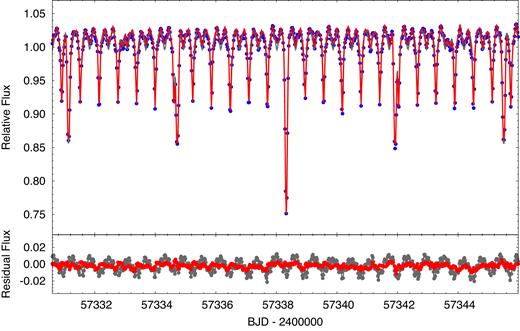
A zoomed-in ∼14-d segment of the K2 flux data showing the superposition of the eclipses of the A and B binaries. The data are shown in blue, the grey curve is a pure, double blended EB model fit, while the red curve is the net model fit taking into account both the binary and the other distortion effects (see text for details). The residuals of the data from the two models are shown in the bottom panel.
The disentangled and folded light curve of each binary is shown separately in Fig. 2. These plots demonstrate the likely semidetached nature of the 0.618-d binary and the detached nature of the 3.595-d binary.
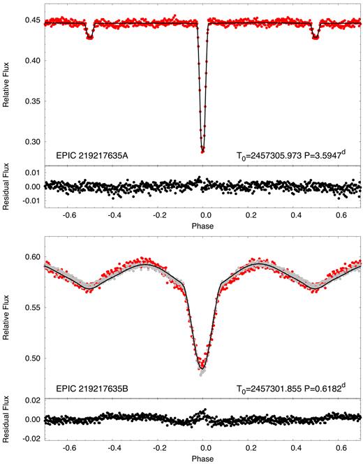
The disentangled and folded light curves of the 3.595-d ‘A’ binary and the 0.618-d ‘B’ binary (red dots). The black curves represent the disentangled, folded light curves, obtained from the simultaneous light-curve solution (partially shown in Fig. 1). In the case of binary B the grey dots represent the sum of the disentangled, folded light curve and a simple model of the rotational spot modulation (see text for details). The bottom panel for each binary shows the folded, disentangled residuals of the full K2 data from the model fit.
We return to a more detailed quantitative analysis of the light curves of the two binaries in Section 7. To start, we simply collect the available photometry on the target-star image in Table 1. Note that these magnitudes refer to the combined light from all four stars in both binaries.
Properties of the EPIC 219217635 system.
| RA (J2000) | 18:59:00.625 |
|---|---|
| Dec. (J2000) | −17:15:57.13 |
| Kp | 12.72 |
| Bb | 13.86 |
| ga | 13.42 |
| Vb | 13.13 |
| Rb | 11.74 |
| ra | 12.72 |
| |$z$|a | 13.42 |
| ib | 12.43 |
| Jc | 11.44 |
| Hc | 11.11 |
| Kc | 11.02 |
| W1d | 10.58 |
| W2d | 10.61 |
| W3d | 10.79 |
| W4d | ... |
| Distance (pc)e | 870 ± 100 |
| μα (mas yr−1)f | −1.9 ± 1.5 |
| μδ (mas yr−1)f | −7.1 ± 2.4 |
aTaken from the Sloan Digital Sky Survey (SDSS) image (Ahn et al. 2012 ).
bFrom VizieR http://vizier.u-strasbg.fr/; Fourth U.S. Naval Observatory CCD Astrograph Catalog (UCAC4; Zacharias et al. 2013).
cTwo Micron All Sky Survey (2MASS) catalogue (Skrutskie et al. 2006).
dWide-field Infrared Survey Explorer (WISE) point source catalogue (Cutri et al. 2013).
eBased on photometric parallax only (see Section 7). This utilized an adapted V magnitude of 13.1.
3 ADAPTIVE OPTICS IMAGING
We obtained Keck II/Near-Infrared Camera 2 (NIRC2; PI: Keith Matthews) observations of the target star EPIC 219217635 on 2017 May 10ut using the narrow camera (10 × 10 arcsec2 field of view) to better characterize this quadruple system. Our observations used the target star as the guide star and dome flat-fields and dark frames to calibrate the images and remove artefacts.
We used a three-point dither pattern to acquire twelve 8-s frames of EPIC 219217635 in the Ks band (central wavelength 2.145 |$\mu$|m), for a total on-sky integration time of 96 s. Fig. 3 shows a stacked Ks band image of this target The top panel shows the full AO image that covers 13 × 13 arcsec2 on the sky, and includes three of the neighbour stars (labelled C1, C2, and C3), which are likely to be background stars rather than gravitationally bound companions. The AO photometry for the three nearby stars is given in Table 2. Because of the large separations of these neighbour stars, C1 only appears in two out of the three dither positions, while C2 and C3 appear in only one out of three dither positions. The Ks band astrometry was computed via point spread function (PSF) fitting using a combined Moffat and Gaussian PSF model following the techniques described in Ngo et al. (2015) and the NIRC2 narrow camera plate scale and distortion solution presented in Service et al. (2016).
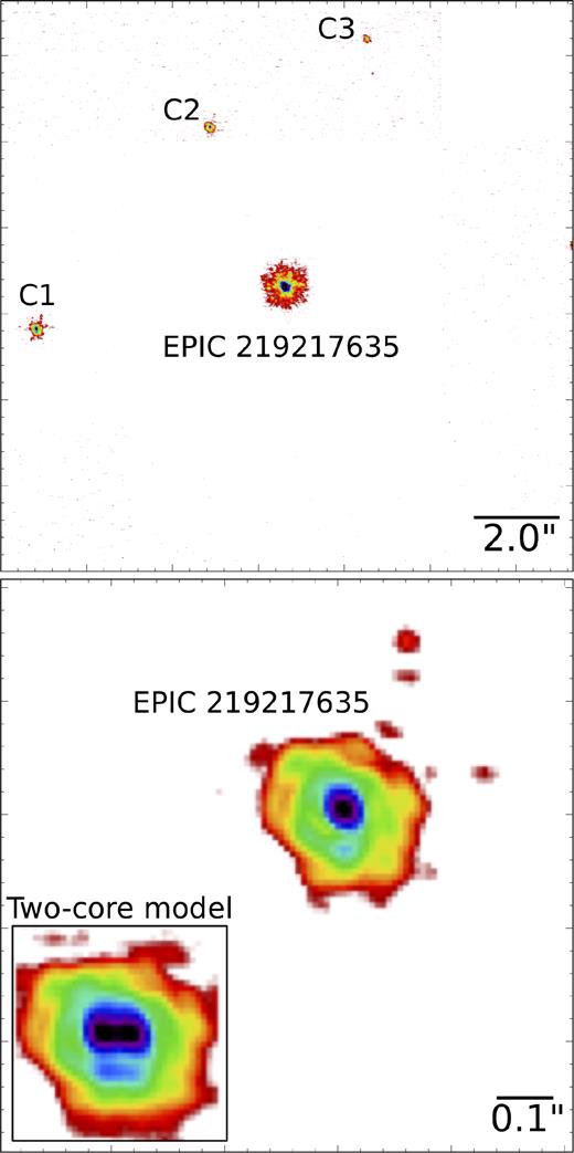
Keck AO image in Ks band of EPIC 219217635. Top panel: full image covering ∼13 × 13 arcsec2. Three of the neighbouring stars are labelled C1, C2, and C3 for reference. Bottom panel: zoom-in around the target star EPIC 219217635. The inset shows a simple simulation of what the image would look like if the two binaries were separated by 0.05 arcsec (see text for a description of how this was generated). We conclude that the two binaries in this target image are clearly unresolved at the 0.05 arcsec level.
Stellar neighbours of EPIC 219217635a.
| Star | Flux ratio | Separation | Pos. angle | |$t_{{{\rm exp}}}^{b}$| |
|---|---|---|---|---|
| (Ks band) | (mas) | (deg E of N) | (s) | |
| C1 | 5.18 ± 0.11 | 5873 ± 2.9 | 99.53 ± 0.03 | 64 |
| C2 | 11.49 ± 0.58 | 4087 ± 2.2 | 25.08 ± 0.03 | 32 |
| C3 | 29.75 ± 0.74 | 6036 ± 3.0 | 341.39 ± 0.03 | 32 |
aResults obtained from the Keck AO image.
bTotal exposure time on each neighbour star. While the target star was present for the full 96 s of integration, the neighbour stars only appeared in-frame for a subset of the dither positions.
In the bottom panel of Fig. 3, we show a zoomed-in image of the target star. This blown-up image looks distinctly single, and shows no sign of the core even being elongated. We have carried out simulations of close pairs of comparably bright images, at a range of spacings, and we conclude from this that separations between the two binaries of ≳0.05 arcsec can be conservatively ruled out. At a source distance of some 870 pc, this sets an upper limit on the projected physical separation of ∼50 au.
A simple demonstration of what the AO image would look like if the two binaries (of nearly equal brightness; see Section 7) were separated by 0.05 arcsec in the horizontal direction is shown in the inset to the bottom panel in Fig. 3. To generate the inset figure, we simply duplicated the zoomed-in AO image, shifted it by 0.05 arcsec in the horizontal direction, and added it to the original image. One can see that if the two binaries were indeed separated by 0.05 arcsec, the core of the image would be noticeably elongated.
4 GROUND-BASED PHOTOMETRY
4.1 HAO observations
The Hereford Arizona Observatory (HAO) consists of a 0.34-m Meade brand Schmidt–Cassegrain Telescope (SCT) on a fork mount, inside an ExploraDome. All hardware is controlled via buried cables from a nearby residence. maxim dl 5.2 software is used to control the telescope, dome, focuser, filter wheel, and SBIG ST-10XME CCD camera. The unbinned image scale was 0.52 arcsec pixel−1. All observations were made using a V-band filter, with exposure times of 60 s. Images were calibrated using master bias, dark and flat images. 10 reference stars and seven calibration stars were employed for converting instrument magnitude to V magnitude.
4.2 PEST observations
Perth Exoplanet Survey Telescope (PEST) is a home observatory with a 12-inch Meade LX200 SCT f/10 telescope with a SBIG ST-8XME CCD camera. The observatory is owned and operated by Thiam-Guan (TG) Tan. PEST is equipped with a BVRI filter wheel, a focal reducer yielding f/5, and an Optec TCF-Si focuser controlled by the observatory computer. PEST has a 31× 21 arcmin2 field of view and a 1.2 arcsec pixel−1 scale. PEST is located in a suburb of the city of Perth, Western Australia. PEST observed EPIC 219217635 on 7 nights between 2017 June 5 and 2017 August 23 in the V band with 120-s integration times.
In all, the HAO and PEST observations led to measurements of four precise primary eclipse times for the 3.595-d ‘A’ binary and an equal number of primary eclipses for the 0.618-d ‘B’ binary (see the last column of Tables 3 and 4). Additionally, on the night of 2017 June 12 an event involving an overlapping primary eclipse of binary A and a secondary eclipse of binary B was also observed at PEST Observatory. However, due to the composite nature of this eclipse we were not able to determine the mid-eclipse times with satisfactory accuracies and, therefore, we did not tabulate this event.
Mid-times of primary eclipses of EPIC 219217635A.
| BJD | Cycle | Std. dev. | BJD | Cycle | Std. dev. | BJD | Cycle | Std. dev. |
|---|---|---|---|---|---|---|---|---|
| − 240 0000 | no. | (d) | − 240 0000 | no. | (d) | − 240 0000 | no. | (d) |
| 57302.37640 | −1.0 | 0.00057 | 57334.73057 | 8.0 | 0.00012 | 57367.08298 | 17.0 | 0.00129 |
| 57305.97293 | 0.0 | 0.00014 | 57338.32397 | 9.0 | 0.00022 | 57370.67604 | 18.0 | 0.00019 |
| 57309.56653 | 1.0 | 0.00018 | 57341.92041 | 10.0 | 0.00016 | 57374.27121 | 19.0 | 0.00019 |
| 57313.16229 | 2.0 | 0.00019 | 57345.51450 | 11.0 | 0.00017 | 57377.86827 | 20.0 | 0.00173 |
| 57316.75708 | 3.0 | 0.00020 | 57349.10967 | 12.0 | 0.00017 | 57381.46098 | 21.0 | 0.00012 |
| 57320.35134 | 4.0 | 0.00019 | 57352.70271 | 13.0 | 0.00046 | 57891.91419 | 163.0 | 0.00009 |
| 57323.94668 | 5.0 | 0.00022 | 57356.29934 | 14.0 | 0.00031 | 57924.26923 | 172.0 | 0.00010 |
| 57327.54058 | 6.0 | 0.00018 | 57359.89390 | 15.0 | 0.00011 | 57942.24434 | 177.0 | 0.00020 |
| 57331.13552 | 7.0 | 0.00039 | 57363.48917 | 16.0 | 0.00022 | 57988.97864 | 190.0 | 0.00025 |
Note. Most of the eclipses (cycle nos −1 to 21) were observed by Kepler spacecraft. Last four eclipses (under the horizontal line) were observed at HAO (no. 163) and PEST (nos 172−190) observatories.
Mid-times of primary eclipses of EPIC 219217635B.
| BJD | Cycle | Std. dev. | BJD | Cycle | Std. dev. | BJD | Cycle | Std. dev. |
|---|---|---|---|---|---|---|---|---|
| − 240 0000 | no. | (d) | − 240 0000 | no. | (d) | − 240 0000 | no. | (d) |
| 57301.85339 | 0.0 | 0.00055 | 57329.67001 | 45.0 | 0.00027 | 57357.49055 | 90.0 | 0.00043 |
| 57303.08879 | 2.0 | 0.00020 | 57330.28886 | 46.0 | 0.00107 | 57358.72688 | 92.0 | 0.00047 |
| 57303.70704 | 3.0 | 0.00045 | 57330.90695 | 47.0 | 0.00022 | 57359.34632 | 93.0 | 0.00036 |
| 57304.32550 | 4.0 | 0.00027 | 57331.52407 | 48.0 | 0.00039 | 57360.58266 | 95.0 | 0.00050 |
| 57304.94365 | 5.0 | 0.00027 | 57332.14301 | 49.0 | 0.00007 | 57361.20038 | 96.0 | 0.00012 |
| 57305.56253 | 6.0 | 0.00152 | 57332.76132 | 50.0 | 0.00025 | 57362.43609 | 98.0 | 0.00067 |
| 57306.18046 | 7.0 | 0.00003 | 57333.37931 | 51.0 | 0.00083 | 57363.05545 | 99.0 | 0.00047 |
| 57306.79734 | 8.0 | 0.00071 | 57333.99694 | 52.0 | 0.00061 | 57363.67455 | 100.0 | 0.00061 |
| 57307.41647 | 9.0 | 0.00048 | 57334.61525 | 53.0 | 0.00014 | 57364.29122 | 101.0 | 0.00017 |
| 57308.03398 | 10.0 | 0.00091 | 57335.23419 | 54.0 | 0.00078 | 57364.91057 | 102.0 | 0.00114 |
| 57308.65247 | 11.0 | 0.00076 | 57335.85254 | 55.0 | 0.00026 | 57365.52781 | 103.0 | 0.00080 |
| 57309.27014 | 12.0 | 0.00022 | 57337.08857 | 57.0 | 0.00031 | 57366.14836 | 104.0 | 0.00045 |
| 57309.88869 | 13.0 | 0.00108 | 57337.70643 | 58.0 | 0.00032 | 57366.76422 | 105.0 | 0.00031 |
| 57310.50691 | 14.0 | 0.00012 | 57338.94273 | 60.0 | 0.00006 | 57367.38405 | 106.0 | 0.00077 |
| 57311.12496 | 15.0 | 0.00055 | 57339.56161 | 61.0 | 0.00011 | 57368.00177 | 107.0 | 0.00084 |
| 57311.74309 | 16.0 | 0.00007 | 57340.79859 | 63.0 | 0.00075 | 57368.62095 | 108.0 | 0.00047 |
| 57312.36134 | 17.0 | 0.00009 | 57342.03502 | 65.0 | 0.00036 | 57369.23842 | 109.0 | 0.00038 |
| 57312.97808 | 18.0 | 0.00032 | 57342.65434 | 66.0 | 0.00089 | 57369.85815 | 110.0 | 0.00200 |
| 57313.59722 | 19.0 | 0.00026 | 57343.27132 | 67.0 | 0.00023 | 57370.47323 | 111.0 | 0.00026 |
| 57314.21555 | 20.0 | 0.00036 | 57343.89018 | 68.0 | 0.00025 | 57371.09366 | 112.0 | 0.00041 |
| 57314.83386 | 21.0 | 0.00009 | 57344.50773 | 69.0 | 0.00024 | 57371.71162 | 113.0 | 0.00039 |
| 57315.45107 | 22.0 | 0.00316 | 57345.12682 | 70.0 | 0.00090 | 57372.33037 | 114.0 | 0.00067 |
| 57316.07058 | 23.0 | 0.00034 | 57345.74510 | 71.0 | 0.00041 | 57372.94706 | 115.0 | 0.00044 |
| 57317.30683 | 25.0 | 0.00010 | 57346.36355 | 72.0 | 0.00078 | 57373.56618 | 116.0 | 0.00028 |
| 57317.92490 | 26.0 | 0.00070 | 57346.98041 | 73.0 | 0.00011 | 57374.80215 | 118.0 | 0.00045 |
| 57319.16173 | 28.0 | 0.00057 | 57347.59947 | 74.0 | 0.00042 | 57375.41912 | 119.0 | 0.00070 |
| 57321.01640 | 31.0 | 0.00040 | 57348.21883 | 75.0 | 0.00107 | 57376.65586 | 121.0 | 0.00086 |
| 57321.63400 | 32.0 | 0.00006 | 57348.83568 | 76.0 | 0.00023 | 57377.27327 | 122.0 | 0.00047 |
| 57322.87125 | 34.0 | 0.00014 | 57349.45359 | 77.0 | 0.00013 | 57378.51223 | 124.0 | 0.00009 |
| 57323.48879 | 35.0 | 0.00046 | 57350.07298 | 78.0 | 0.00040 | 57379.12853 | 125.0 | 0.00041 |
| 57324.10676 | 36.0 | 0.00063 | 57350.69137 | 79.0 | 0.00037 | 57380.36682 | 127.0 | 0.00074 |
| 57324.72549 | 37.0 | 0.00035 | 57351.30971 | 80.0 | 0.00014 | 57380.98310 | 128.0 | 0.00066 |
| 57325.34337 | 38.0 | 0.00029 | 57351.92734 | 81.0 | 0.00137 | 57381.60127 | 129.0 | 0.00047 |
| 57325.96183 | 39.0 | 0.00059 | 57352.54397 | 82.0 | 0.00022 | 57382.21900 | 130.0 | 0.00029 |
| 57326.57965 | 40.0 | 0.00053 | 57353.78200 | 84.0 | 0.00037 | 57910.16115 | 984.0 | 0.00013 |
| 57327.19787 | 41.0 | 0.00034 | 57355.01923 | 86.0 | 0.00029 | 57923.14305 | 1005.0 | 0.00015 |
| 57327.81569 | 42.0 | 0.00039 | 57355.63804 | 87.0 | 0.00178 | 57924.38240 | 1007.0 | 0.00023 |
| 57328.43373 | 43.0 | 0.00034 | 57356.87288 | 89.0 | 0.00035 | 57929.32426 | 1015.0 | 0.00013 |
| 57329.05172 | 44.0 | 0.00054 |
Note. Most of the eclipses (cycle nos 0−130) were observed by Kepler spacecraft. Last four eclipses (under the horizontal line) were observed at the PEST Observatory.
5 PERIOD STUDY
In order to look for and analyse the possible eclipse timing variations (ETVs) in the two binaries, we determined the times of each eclipse minimum using the K2 data with the blended binaries in the following manner. First we formed a folded, binned light curve with the period of the 0.618-d binary B in such a way that the narrow region around the primary and secondary eclipses of the 3.595-d binary A was omitted. Then, the profile of the primary eclipse of this folded light curve (lower panel of Fig. 2) was used as a template for calculating the times of the primary eclipses of binary B in the K2 data set. (We decided not to utilize the secondary eclipses, due to the fact that they are rather shallow.)
In order to obtain the times of the primary eclipses of binary A, we removed the folded, binned, averaged binary B light curve from the K2 data set with the use of a three-point local Lagrange interpolation. Then, this disentangled light curve (upper panel of Fig. 2) was used both for forming the folded, binned, averaged light curve of binary A, and also for determining the times of the primary eclipses of binary A. (Here, for the same reasons as mentioned above, we utilized only the times of the primary eclipses.)
In such a way we obtained the first iteration K2 ETV curves for both binaries. Later, however, during our analysis, we realized that besides the classical binary light-curve variations, the light curve also exhibits some additional periodic variations (see Section 7). Thus, after the separation and removal of these extra periodic signals from the K2 light curve, we repeated the process described above, and we were able to refine the ETV curves (see Figs 4 and 5, and also Tables 3 and 4).
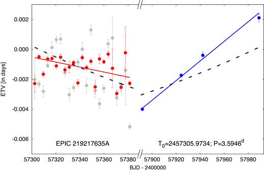
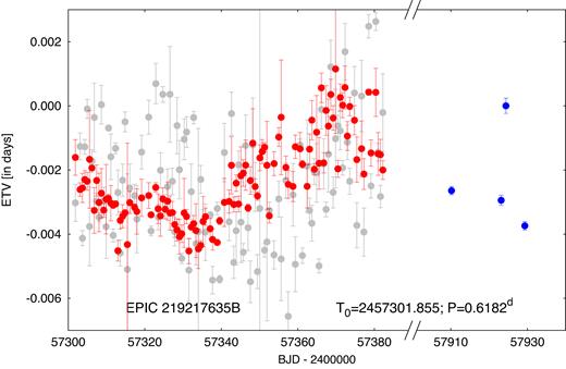
ETVs of binary A. Grey and red circles represent eclipse times determined from the K2 observations before and after the removal of non-binary light-curve variations, respectively. Blue data points represent the ground-based timing measurements. Red and blue lines are linear fits to the red and blue ETV points, respectively, which would illustrate two constant-period segments with a period difference of 26 s (note in particular the broken time axis). Black dashed lines illustrate the two sections of a parabola that result from a quadratic fit to the red and blue ETV points together, i.e. modelling a constant rate of increase in the orbital period.
ETVs of binary B. Grey and red circles represent eclipse times determined from the K2 observations before and after the removal of light-curve variations, respectively, that are not inherent to the binary light curve. Blue data points represent the ground-based timing measurements. Note the broken time axis between the two sets of observations.
Furthermore, we have carried out ground-based photometric follow-up observations with two telescopes on 8 nights between 2017 May and August (see Section 4). We were thereby able to determine eight additional primary eclipse times (four for both binaries; given at the end of Tables 3 and 4), which made it possible to extend significantly the observing window and to check for longer time-scale trends in the period variations of the two binaries. In order to determine the ground-based eclipse times, we first converted these observations to the flux regime and then used the same K2 template eclipse profiles as before. Furthermore, in the case of the binary A eclipses we removed the ellipsoidal light variations (ELVs) of binary B via the use of the folded, disentangled binary B K2 light curve after phasing it according to its expected phase at the epoch of the ground-based observations.
Regarding the eclipse timings of binary A (Fig. 4) no definitive short-term ETVs can be seen during the 80 d of the K2 observations. The constant binary period is found to be |$P_{\rm A\hbox{-}K2}=3{^{\rm d}_{.}}59469\pm 0{^{\rm d}_{.}}00002$|. On the other hand, the four ground-based eclipse times (which span a similar time interval) do not phase up to the K2 data. Fitting a constant period to the four ground-based data points yields |$P_{\rm A\hbox{-}2017}=3{^{\rm d}_{.}}59499\pm 0{^{\rm d}_{.}}00001$| that differs by ∼25.6 s from the K2 period (at the 12σ level). We also fit the joint K2 and 2017 ground-based data using a quadratic ephemeris (see black, dashed segments of the corresponding parabola in Fig. 4). A parabolic ETV represents a linear period variation during the 1.9-yr span of both sets of observations. As one can see, the parabolic fit is quite poor. The resultant period variation rate is found to be ΔP = 1.4 ± 0.3 × 10⁻⁶d cycle−1 or, |$\dot{P}/P=4.0\pm 0.8\times 10^{-5}\,{\rm yr}^{-1}$|. Assuming that the source of this period variation was Keplerian orbital motion of the binary around the centre of mass of the quadruple system, one can convert this quantity into a variation in the systemic RV of binary A, as |$\dot{\gamma }_\mathrm{ A} \approx c\Delta P/P^2$|, which results in |$\dot{\gamma }_\mathrm{ A} \simeq 0.038\pm 0.008\,{\rm cm\,s}^{-2}$|. As we find later, this value is an order of magnitude higher than we find directly from our RV study (see Section 6).
We turn now to the ETV curve for binary B (see Fig. 5). In this case the K2 data, after the removal of the non-binary light-curve variations, clearly reveal short-term, non-linear behaviour in the timing data. On the other hand, however, this non-linear trend, which would correspond to an increasing orbital period, obviously did not continue all the way to the time of the ground-based observations. These latter measurements are in conformity with a constant average period since the beginning of the K2 observations.
Speculating on the origin of these period variations, we can only state with certainty that none of them could arise from the orbit of the two binaries around each other. First, there is the evident contradiction between the period variations found in binary A and the directly measured value of |$\dot{\gamma }_\mathrm{ A}$| found for binary A (see Section 6). Second, there is also the fact that, according to our combined RV and light-curve solution (see Section 7), the total mass of each of the two binaries is similar and, therefore, the ETVs arising from the orbits of the two binaries forming the quadruple system should be similar in amplitude and opposite in phase.4 In the case of binary B, the spotted nature of at least one of the stars might offer a plausible explanation for the observed short-term ETVs, as similar behaviour has been reported for several spotted Kepler binaries (see e.g. Tran et al. 2013; Balaji et al. 2015).
In the case of binary A, an interpretation of the observed ETV behaviour will require further observations.
6 NOT-FIES RADIAL VELOCITY STUDY
We obtained 20 spectra of EPIC 219217635 employing the Nordic Optical Telescope (NOT) and its FIbre-fed Echelle Spectrograph (FIES; Frandsen & Lindberg 1999; Telting et al. 2014) in high-resolution mode (R∼ 67 000). The spectra have been taken between 2016 May 18 and 2017 July 5 with exposure times ranging between 20 and 35 min. Each science exposure was accompanied by one ThAr exposure immediately prior to wavelength calibration.
The data reduction was carried out using fiestool.5 In the following we used the wavelength-calibrated extracted, but not order-merged spectra. Cosmic rays have been identified and removed, the blaze function of the spectrograph was accounted for using flat-field exposures, and the spectra have been normalized. For the purpose of obtaining RVs we focus on the spectral region between 4500 and 6700 Å. At shorter wavelengths the typical signal-to-noise ratio (S/N) per spectral bin is below 3 for the combined spectrum of the two binaries. At longer wavelengths few stellar lines are present. We created cross-correlation functions (CCFs) for each spectral order of each observation using a template obtained from the phoenix library (Husser et al. 2013). Specifically we used the phoenix model with Teff = 6500 K, log g = 4.0, and solar metallicity. We checked if using different templates with somewhat different parameters changes the RV we derive (see below), which is not the case.
Next we fitted two Gaussians to the CCF of each observation obtained by simple summation of all CCFs from the different orders. One Gaussian has a small σ of 11 km s−1 representing the primary from binary A. The second Gaussian with σ = 120 km s−1 represents the primary from binary B. The positions of these Gaussians are interpreted as RVs of the two primary components. We estimate the uncertainties in these RVs using the following approach. The CCFs from the different spectral orders are grouped into four different wavelength regions. RVs for each of the four different orders are obtained in the same way as for the CCFs from the complete spectral region and the standard deviation about the mean is used as the RV uncertainty.
The RV plots obtained with the NOT-FIES spectrometer are shown in Fig. 6, and the individual RV measurements are listed in Table 5. The RV curve for the primary star in binary A (top panel) has very well determined parameter values with a typical uncertainty per RV point of ∼0.5 km s−1. The orbital amplitude, KA, is 61.28 ± 0.15 km s−1, while the system velocity is γA = 30.91 ± 0.13 km s−1. For the primary component in binary B (bottom panel), the typical uncertainties per RV point are ∼12 km s−1. The corresponding elements are KB = 64.1 ± 3.6 km s−1 and γB = 32.3 ± 2.2 km s−1. These were all for assumed circular orbits, but we fit for, and set constraints on, eccentric orbits as well.
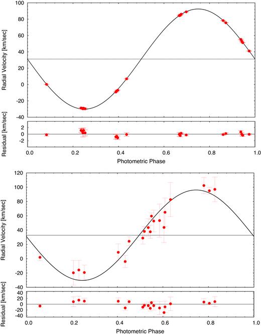
Folded RV curves for the 3.595-d ‘A’ binary (top panel) and the 0.618-d ‘B’ binary (bottom panel). The black curves are the best-fitting circular orbit models. For a better visualization all the individual observed and model data points are corrected for the non-zero |$\dot{\gamma }$| values, i.e. we plot the |$v_{\rm corr}=v_{\rm obs/mod}-\dot{\gamma } (t_{\rm obs/mod}-t_0)$| data.
Radial velocity studya.
| RV measurements BJD – 240 0000 | Binary A km s−1 | Binary B km s−1 |
|---|---|---|
| 57526.6406 | −9.40 ± 0.73 | +55.8 ± 23 |
| 57526.6554 | −8.01 ± 0.64 | +67.3 ± 20 |
| 57526.6703 | −7.20 ± 0.55 | +85.1 ± 24 |
| 57527.6428 | +84.09 ± 0.59 | −17.3 ± 17 |
| 57527.6576 | +84.45 ± 0.35 | −13.4 ± 13 |
| 57527.6725 | +85.91 ± 0.16 | −17.0 ± 10 |
| 57528.6155 | +55.04 ± 0.41 | +104.7 ± 11 |
| 57528.6303 | +52.84 ± 0.51 | +97.4 ± 5 |
| 57528.6452 | +51.01 ± 0.26 | +99.3 ± 17 |
| 57529.6858 | −28.91 ± 0.60 | +31.2 ± 8 |
| 57529.7006 | −29.18 ± 0.77 | +45.8 ± 12 |
| 57529.7155 | −29.87 ± 1.24 | +55.0 ± 15 |
| 57666.3547 | −29.62 ± 0.91 | +42.7 ± 21 |
| 57669.3399 | +0.31 ± 0.37 | −5.0 ± 8 |
| 57682.3316 | +89.05 ± 0.27 | +23.0 ± 6 |
| 57683.3258 | +41.12 ± 0.19 | +0.53 ± 5 |
| 57864.7275 | +7.46 ± 0.53 | +32.5 ± 7 |
| 57916.5810 | +78.88 ± 0.22 | +1.94 ± 12 |
| 57934.5976 | +76.21 ± 0.26 | +52.1 ± 5 |
| 57939.5396 | −28.29 ± 0.75 | +30.1 ± 9 |
| Orbit fits | ||
| T0 (BJD)b | 245 7625.9007± 0.0012 | 245 7625.801± 0.005 |
| P (d) | 3.59486(4) | 0.61815(2) |
| K (km s−1) | 61.28 ± 0.15 | 64.1 ± 3.6 |
| γ (km s−1) | +30.91 ± 0.13 | +32.3 ± 2.2 |
| e | ≲0.01 | ... |
| |$\dot{\gamma }$| (cm s−2)c | 0.0024 ± 0.0007 | −0.020 ± 0.014 |
| Spectroscopic parametersd | ||
| Teff (K) | 6421 ± 134 | ... |
| log g (cgs) | 4.15 ± 0.16e | ... |
| Fe/H (dex) | −0.03 ± 0.07 | ... |
| |$v$| sin i (km s−1) | 16.7 ± 1 | ... |
| MA1 (M⊙) | |$1.23^{+0.10}_{-0.08}$| | ... |
| RA1 (R⊙) | |$1.39^{+0.31}_{-0.17}$| | ... |
| Age (Gyr) | 2.4 ± 1 | ... |
aCarried out with the NOT-FIES spectrometer.
bTime of the primary eclipse and reference time for P and K.
cParameter fitted to the unfolded RV data set.
dParameters refer to the primary star that contributes |$\gtrsim 90\hbox{ per cent}$| of the light from the A binary.
eDerived from the summed spectra; see Section 6.
We also used the NOT-FIES spectral data to determine some of the properties of the primary star in binary A. The results are given in Table 5 and shown in Fig. 7. After obtaining RVs for the A and B binaries we use the tomography algorithm developed by Bagnuolo & Gies (1991) to separate the spectra. We stack the separated spectra to obtain co-added, high S/N spectra of the A and B binaries. We derive stellar parameters of star A1 from the co-added spectrum. Within the spectroscopic framework iSpec (Blanco-Cuaresma et al. 2014), we fit synthetic spectra computed using spectrum (Gray & Corbally 1994) and atlas9 atmospheres (Castelli & Kurucz 2004) to the wavelength region 5000–5500 Å. The spectroscopically determined parameters are listed in Table 5. We derive the stellar mass, radius, and age by fitting spectroscopic constraints (Teff, log g, [Fe/H]) to a grid of a Bag of Stellar Tracks and Isochrones (BaSTI) isochrones (Pietrinferni et al. 2004) using the Bayesian Stellar Algorithm (basta; Silva Aguirre et al. 2015), see Table 5.
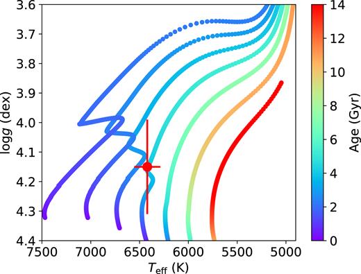
The spectroscopically determined location (with uncertainties) of star A1 in the log g−Teff plane. The coloured curves are evolution tracks for stars of mass 0.9–1.5 M⊙ (increasing from left to right) in steps of 0.1 M⊙. Tracks are colour coded according to the isochrones of stellar evolution time. See text for details.
In Fig. 7, we show the location (with uncertainties) of star A1 in the log g−Teff plane. Superposed on the plot are evolution tracks for stars of mass 0.9–1.5 M⊙ (mass increases from left to right) in steps of 0.1 M⊙. Moreover, the tracks are colour coded according to the isochrones of stellar evolution time.
The lines of the primary star in binary B were too broad (|$v$| sin i≈ 120 km s−1) to allow for a similar analysis.
7 SIMULTANEOUS LIGHT-CURVE AND RV-CURVE MODELLING
We carried out a simultaneous analysis of the blended light curves of the two EBs, and the two radial velocity curves of the primaries of the two EBs using our light-curve emulator code lightcurvefactory (Borkovits et al. 2013; Rappaport et al. 2017). This code employs a Markov chain Monte Carlo (MCMC)-based parameter search, using our own implementation of the generic Metropolis–Hastings algorithm (see e.g. Ford 2005). The basic approach and steps for this study are similar to that which was followed during the previous analysis of the quadruple system EPIC 220204960, described in Rappaport et al. (2017, section 7). Therefore, here we concentrate mainly on the differences compared to this previous work.
7.1 New features of the analysis
First, for a more accurate modelling of the strong ELV effect in the light curve of binary B (see Fig. 2), we implemented the Roche-equipotential-based stellar surface calculations into our code (see e.g. Kopal 1989; and Avni 1976; Wilson 1979, for a formal extension to eccentric orbits and asynchronous stellar rotation). Furthermore, we included an additional switch in the code to set the size parameter of one star (or both) so that it would exactly fill its Roche lobe. In such a way we were able to model the semidetached configuration of binary B.
Second, because our code is now able to fit light-curve photometry, RV, and ETV curves at the same time, we decided to simultaneously analyse the two RV curves along with the blended light curve.
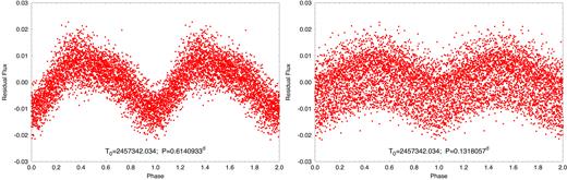
Folded light curves for periods of 0.6141 and 0.1318 d (left and right, respectively) after the best-fitting orbital light curves of the A and B binaries have been subtracted. The period in the left-hand panel is shorter than the orbital period of binary B by only ∼5.75 min. We interpret this as star-spots from the B binary that are not quite corotating with the orbital period of 0.6182 d.
The five most significant peaks of the period analysis of the residual light curve.
| Frequency | Amplitude | Phase | ||
|---|---|---|---|---|
| (d−1) | (×PB) | (×10−3 flux) | (rad) | |
| |$f_1^a$| | 1.628417(1) | 1.00669 | 7.520(1) | −1.2098 |
| |$f_2^a$| | 7.586925(1) | 4.69175 | 3.217(1) | −1.2443 |
| |$f_3^a$| | 3.257062(1) | 2.01352 | 2.128(1) | −0.1286 |
| f4 | 6.102445(1) | 3.77375 | 1.784(1) | −2.7261 |
| f5 | 18.119794(1) | 11.20528 | 1.352(1) | −0.8596 |
aThe frequencies used for the light-curve fitting process.
7.2 Significance of the simultaneous analysis
Furthermore, we also wish to point out that the joint photometric analysis of the two binaries inherently carries some information about the mass ratio of the two binaries and the temperature ratio of the primary star in each binary (TA1/TB1). Since it turns out that there is already sufficient information to adequately determine all the masses in the system, this means that equation (A3) effectively yields TA1/TB1. Therefore, if TA1 is known, one can also find TB1 and then, naturally, the effective temperatures of all four stars can also be obtained. Since it is conceptually interesting that the photometry does encode combined information about the mass ratio of the two binaries and TA1/TB1, we provide a brief discussion of this in Appendix A.
7.3 Fitted parameters and assumptions
As discussed above, all of the astrophysically important parameters of both binaries can be obtained from the same simultaneous analysis, except for the mass, mA1, and the effective temperature, TA1, of the primary of binary A. However, because TA1 and its uncertainty are directly known from the spectroscopic analysis, the only remaining task is to find one additional reasonable constraint to close the system of equations. As a good approximation for mA1 we use the value and uncertainty for mA1 obtained indirectly from the spectroscopic data, as was described in Section 6.
Turning now to the practical implementation of the combined analysis, we note that in most of the runs we adjusted 20–22 parameters. These are as follows.
2 × 3 orbital parameters: the two periods (PA, B), inclinations (iA, B), and reference primary eclipse times (T0, A, B). (Note, in some runs we allowed for an eccentric orbit in binary A and, therefore, the eccentricity, eA, and argument of periastron, ωA, of binary A were also adjusted, but we did not detect any significant, non-zero eccentricity. Thus, for most of the runs we simply adopted circular orbits for both binaries.)
2 × 3 additional RV curve related parameters: systemic radial velocities (γA, B) and linear accelerations (|$\dot{\gamma }_{\rm A,B}$|),6 and spectroscopic mass functions (f(m2)A, B).
The light-curve related parameters: temperature ratios (T2/T1)A, B and also TB1/TA1; the duration of the primary minima (Δtpri)A, B (see Rappaport et al. 2017, section 7 for an explanation); the ratio of stellar radii in binary A (R2/R1)A; and the extra light (lx).
The mass ratio (qB) of binary B.
Finally, the effective temperature, TA1, and mass, mA1, of the primary of binary A, for which we incorporated Gaussian prior distributions with the mean and standard error set to the values obtained from the spectroscopic solution.
Regarding other parameters, a logarithmic limb darkening law was applied, for which the coefficients were interpolated from the passband-dependent pre-computed tables of the phoebe software7 (Prša & Zwitter 2005). Note that these tables are based on the stellar atmospheric models of Castelli & Kurucz (2004). The gravity darkening exponents were set to their traditional values appropriate for such late-type stars (g = 0.32). We found that the illumination/reradiation effect was negligible for the wider binary A; therefore, in order to save computing time, it was calculated only for the narrower binary B. The Doppler boosting effect was taken into account for both binaries (Loeb & Gaudi 2003; van Kerkwijk et al. 2011).
Furthermore, we assumed that all four stars rotate synchronously with their respective orbits. For the semidetached component of binary B this assumption seems quite natural. On the other hand, some primaries of semidetached systems have been found to be rapid rotators relative to their orbits (see e.g. Wilson 1994, for a review). In our case, however, we may reasonably assume that the highest amplitude peak in the residual light curve (see Table 6 and Fig. 8), with a period that differs by only ∼5–6 min from the orbital period of binary B, has its origin in the rotational modulation of the primary of binary B, which clearly dominates the light contribution of this binary. Thus, it is also reasonable to adopt a synchronous rotation for the primary of binary B. Regarding the detached binary A, the spectroscopically obtained projected rotational velocity of the primary component |$v$| sin i = 16.7 ± 1 km s−1 (see Table 5) offers an a posteriori verification of our assumption since the projected synchronous rotational velocity that can be deduced from our solution is found to be in essentially perfect agreement with this result (see in Table 7, below). Finally, note that we have no information on the rotation of the secondary component of binary A but, due to its small contribution to the total flux of the system, its rotational properties have only a minor influence on our solution.
Parameters from the double EB simultaneous light curve and SB1+SB1 RVs solution.
| Parameter | Binary A | Binary B | ||
|---|---|---|---|---|
| P (d) | 3.594728 ± 0.000014 | 0.618214 ± 0.000005 | ||
| Semimajor axis (R⊙) | 12.21 ± 0.19 | 3.65 ± 0.16 | ||
| i (°) | 89.50 ± 0.58 | 64.66 ± 0.56 | ||
| e | 0 | 0 | ||
| ω (°) | − | − | ||
| tprim eclipse (BJD) | 245 7341.9183± 0.0002 | 245 7342.0357± 0.0003 | ||
| γ (km s−1) | 30.24 ± 0.08 | 27.47 ± 2.44 | ||
| |$\dot{\gamma }$| (cm s−2) | 0.0039 ± 0.0004 | 0.0287 ± 0.0105 | ||
| f(m2) (M⊙) | 0.0863 ± 0.0005 | 0.0173 ± 0.0027 | ||
| Individual stars | A1 | A2 | B1 | B2 |
| Relative quantities | ||||
| Mass ratio (q = m2/m1] | 0.56 ± 0.05 | 0.31 ± 0.03 | ||
| Fractional radiusa (R/a) | 0.0975 ± 0.0014 | 0.0604 ± 0.0014 | 0.3542 ± 0.0077 | 0.2647 ± 0.0077 |
| Fractional luminosity | 0.37602 | 0.0186 | 0.5416 | 0.0254 |
| Extra light [lx] | 0.048 ± 0.030 | |||
| Physical quantities | ||||
| |$T_{\rm eff}^b$| (K) | 6473 ± 129 | 4421 ± 107 | 6931 ± 250 | 4163 ± 176 |
| Massc (M⊙) | 1.21 ± 0.09 | 0.68 ± 0.03 | 1.30 ± 0.21 | 0.41 ± 0.07 |
| Radiusd (R⊙) | 1.19 ± 0.03 | 0.74 ± 0.02 | 1.33 ± 0.06 | 1.04 ± 0.05 |
| Luminosity (L⊙) | 2.24 ± 0.20 | 0.19 ± 0.02 | 3.66 ± 0.61 | 0.29 ± 0.06 |
| Mbol | 3.87 ± 0.10 | 6.56 ± 0.12 | 3.33 ± 0.19 | 6.09 ± 0.22 |
| log g (cgs) | 4.37 ± 0.04 | 4.53 ± 0.02 | 4.33 ± 0.09 | 4.10 ± 0.09 |
| |$(v\sin i)_{\rm sync}^e$| (km s−1) | 16.8 ± 0.4 | 10.4 ± 0.3 | 95.6 ± 4.8 | 76.9 ± 4.0 |
| (MV)tot | 2.74 ± 0.12 | |||
| Distancef (pc) | 870 ± 100 | |||
aPolar radii.
bTeff, A1 and its uncertainty were taken from the spectroscopic analysis and used as a Gaussian prior for this joint photometric + RV analysis; the other Teffs were calculated from the adjusted temperature ratios.
cmA1 and its uncertainty were taken from the spectroscopic analysis and used as a Gaussian prior; the other masses were calculated as described in Section 7.2.
dStellar radii were derived from the volume-equivalent fractional radii (R/a) and the orbital separation.
eProjected synchronized rotational velocities, calculated using the volume-equivalent radii.
fDistance to the quadruple, calculated from the photometric distance modulus with the inclusion of an estimate of the interstellar extinction.
7.4 Results of the simultaneous analysis
The orbital elements of the two binaries, and the astrophysically relevant parameters of the four stars, together with their uncertainties, are tabulated in Table 7. About half of these quantities were obtained directly from our simultaneous MCMC analysis of the photometric and RV data, while the others were calculated from the MCMC adjusted parameters using the relations discussed above, as well as some additional trivial ones. Examples of the latter include the calculation of the semimajor axes from the stellar masses and periods, and the determination of the volume-equivalent physical radii of the four stars from their fractionalradii.
We also computed the luminosities of the four stars both in solar luminosity (L⊙) and as bolometric absolute magnitudes. We also compute the total absolute visual magnitude (MV)tot of the quadruple system as a whole. For this latter quantity, the bolometric correction for each star was calculated with the formulae of Flower (1996).8 Furthermore, for the calculation of (MV)tot we assumed that the extra light contribution (lx= 0.048 ± 0.030) found in our light-curve solution from the Kepler photometric band is essentially the same as the contaminating light in V band. (However, since it appears that the extra light is fairly negligible, this issue is not very important.) These luminosities and magnitudes are reported inTable 7.
Then, by the use of the observed V magnitude, listed in Table 1, we can estimate a photometric distance to the system. We first calculate the maximum hydrogen column density between us and the quadruple, NH, using NASA’s High Energy Astrophysics Science Archive Research Center (HEASARC) on-line tools9 and find NH ≲ 1.4 × 1021 cm−2. We then used a conversion from NH to AV taken from Guver & Özel (2009): NH ≃ 2.2 × 10²¹ AV. This yields an extinction of AV ≲ 0.63. We also utilized a web-based applet10 to estimate E(B − V) = 0.22 ± 0.03 that we translate to AV = 0.68 ± 0.09. When we propagate the associated uncertainties in all the involved quantities, we find a distance of 870 ± 100 pc; this is also tabulated in the last row ofTable 7.11
A comparison of those astrophysical parameters of the primary star in binary A that were obtained both from the spectroscopic (Table 5), and the combined photometric + RV (Table 7) analysis shows slight but significant discrepancies. In particular, the radius inferred from the joint photometric + RV analysis (|$R_{\rm A1}^{\rm phot}\simeq 1.19\pm 0.03\,{\rm R}_{\odot }$|) is 1.2σspec smaller than the spectroscopically inferred radius (|$R_{\rm A1}^{\rm spec}\simeq 1.39^{+0.31}_{-0.17}\,{\rm R}_{\odot }$|). This leads to an RV + photometric loggA1 that is 0.22 ± 0.16 dex higher than that determined from the spectroscopic analysis.
This slight inconsistency in log gA1 should be considered together with the inferred absolute dimensions of the secondary component of binary A. While the effective temperature (TA2 ≃ 4400 ± 100 K) and mass (mA2 ≃ 0.68 ± 0.03 M⊙) of the secondary are in accord with the main-sequence nature of this star to within the 1σ uncertainty, the inferred stellar radius (RA2 ≃ 0.74 ± 0.02 R⊙) reveals a significantly oversized star for its mass. One might imagine that the inconsistency could readily be resolved assuming that the joint analysis failed to obtain the correct value for the ratio of the relative radii of binary A (r2/r1), which itself was an adjusted parameter. However, we note that the eclipses in binary A were found to be total (i.e. in the sense of four contact points) and, therefore, in this case the ratio of the stellar radii is relatively well determined. This discrepancy did lead us to conduct some further tests, initiating new MCMC runs in which the radius of the secondary of binary A was constrained with the use of the Tout et al. (1996) mass–radius relation. These runs led to significantly worse fits. In particular, that part of the χ2 sum that was calculated exclusively from the light-curve solution was found to be higher by about |${\approx} 8\hbox{--}10\hbox{ per cent}$| in the case of the solutions using a constrained secondary radius. Thus, using all the presently available information on the quadruple, we are able to resolve these discrepancies, but we believe that they are reasonable given the very different inputs, uncertainties, and analyses involved.
Binary B is found to be the more interesting of the two binaries from the perspective of stellar evolution theory. The stellar components of binary B are MB1 ≃ 1.33 ± 0.21 M⊙, RB1 ≃ 1.33 ± 0.06 R⊙ and MB2 ≃ 0.41 ± 0.07 M⊙, RB2 ≃ 1.04 ± 0.05 R⊙. The larger uncertainties in the masses come mainly from the poorer quality RV curve, which did not allow for a well-determined spectroscopic mass function. Note, in particular, the greatly oversized radius of the low-mass secondary star compared to its nominal main-sequence radius. Thus, we provide a separate discussion of the likely evolutionary scenario for this system in Section 9.
8 CONSTRAINTS ON THE QUADRUPLE’S OUTER ORBIT
We now utilize what we have learned about the A and B binaries from the AO imaging, the RV measurements, and the photometric data to place a couple of significant constraints on the outer orbit of the quadruple system. There are five principal results that help to constrain the outer orbit: (1) upper limits on the angular separation, α, of binary A and binary B; (2) the difference in gamma velocities between the two binaries, Δγ ≡ γA − γB; (3) the acceleration of the centre of mass of binary A, |$\dot{\gamma }_\mathrm{ A}$|; (4) upper limits on |$\dot{P}_\mathrm{ A}$| and |$\dot{P}_\mathrm{ B}$| from the photometric ETV curves; and (5) the inferred masses of all four stars in the binaries. It turns out that the limits on |$\dot{P}$| (item 4) are not significant compared to essentially the same constraint set by |$\dot{\gamma }_\mathrm{ A}$|, and we do not consider this any further.
The specific values of these constraints are as follows:
α< 0.05 arcsec;
Δγ ≡ γA − γB = −1.4 ± 2.2 km s−1;
|$\dot{\gamma }_{\mathrm{ A}} = 0.0024 \pm 0.0007$| cm s−2;
MA = 2.00 ± 0.06 M⊙ and MB = 1.88 ± 0.06 M⊙.
We hereafter consider the masses of the A and B binaries to be the same to within their statistical uncertainties.
There are five parameters of the outer orbit we would like to know (a, P, e, ω, and i), and only the four constraints listed above. Therefore, we will be able to set only ranges of acceptable values for some of these five parameters. The masses are used to relate a and P through Kepler’s third law.
The approach we take to compute probability distributions for P, e, ω, and i is via Monte Carlo sampling of these parameters, as well as of the unknown instantaneous true anomaly, and then testing for each system realization whether the constraints for α, Δγ, and |$\dot{\gamma }_\mathrm{ A}$| are satisfied to within their uncertainties, assuming Gaussian errors. For each realization, we randomly sample the mean anomaly in time, compute the corresponding eccentric anomaly, and from that the true anomaly, ϕ. Specifically we choose linear random values of P from 0 to 1000 yr, e from 0 to 1, and ω from 0 to 2π. The orbital inclination was chosen from a uniform probability per unit solid angle. Finally, the distance to the source was taken to be 870 pc with a Gaussian distribution with σ = 100 pc. The quantities α, Δγ, and |$\dot{\gamma }_\mathrm{ A}$| are then evaluated via equations (3), (4), and (5) and are compared to the measured values.
Somewhat as we anticipated, the only outer orbit parameters for which interesting constraints could be set are P and a. Output histograms for P and a are shown in Fig. 9. For these two distributions we find that the outer period is most probably near 20 yr, but could reasonably be as short as 10 yr or as long as 80 yr. The corresponding semimajor axis of the quadruple is likely 18 ± 10 au. Therefore, in just a couple of additional seasons of either eclipse monitoring or follow-up RVs from this system, we can expect to see a significant LTTE from the orbit and/or a much more significant determination of |$\dot{\gamma }_\mathrm{ A}$|.
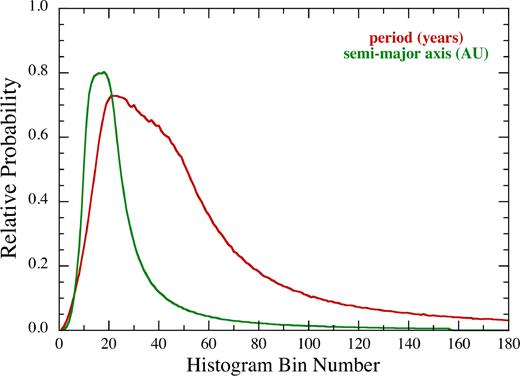
Output histograms for the period and semimajor axis associated with the outer orbit of the quadruple. See text, Section 8 for details of the Monte Carlo orbit sampling.
9 EVOLUTION OF BINARY B
In this section we address the fact that the lower mass star in binary B appears to be the more evolved one. This implies that it is an Algol-like system and the lower mass star either has lost, or is continuing to lose, its envelope to the currently more massive star.
Since the properties of the components in binary B are reasonably well determined, this allows us to construct evolutionary scenarios that are self-consistent with the formation and evolution of EPIC 219217635 as a whole. Given the donor star’s mass (0.41 ± 0.07 M⊙) and radius (≃1.04 ± 0.05 R⊙) we conclude that the star is too large for its mass to be on the main sequence, and therefore must be substantially evolved. In fact, we believe that this star belongs to a class of stars known as ‘stragglers’ that have been previously studied by Kaluzny (2003), Orosz & van Kerkwijk (2003), and Mathieu et al. (2003). These stars are considerably redder than their main-sequence counterparts and likely experienced some nuclear burning before undergoing a phase of rapid mass loss (Case AB evolution). Thus red stragglers can be legitimately viewed as a special class of Algol-like binaries.
The general properties and evolution of Algol variables have been well studied (see e.g. Batten 1989, and references therein; Peters 2001). The more massive star in these systems fills its Roche lobe first and undergoes Roche lobe overflow (RLOF). A prolonged phase of stable (and sometimes rapid) mass transfer to the less massive companion often ensues. One of the difficulties in calculating this type of dynamically stable mass transfer arises from the problem of quantifying the degree to which the mass transfer is non-conservative (i.e. to determine the fraction of mass that is lost from the binary during RLOF). As has been shown by Eggleton (2000), a wide range of values is required in order to explain the observations of Algol-like systems (see also Nelson & Eggleton 2001). The secondary usually accretes enough matter so as to cause the mass ratio to become ‘inverted’ leading to a binary that contains a more evolved yet less massive primary star compared to the secondary star (accretor). Algol variables are normally observed as either being detached with both stars underfilling their respective Roche lobes, or semidetached with the donor star still undergoing RLOF. The orbital periods of these binaries typically vary from Porb ≳ 1 d to decades.
Red stragglers are likely low-mass stars that have evolved considerably (e.g. they may have consumed all of their central hydrogen) before filling their Roche lobes and undergoing a reasonably fast phase of thermal time-scale mass transfer to the accretor (see e.g. Zhou et al. 2018, and references therein). The subsequent evolution can be classified with reference to the bifurcation limit (Pylyser & Savonije 1988). If mass is stripped rapidly enough, the binaries will evolve below the bifurcation limit and will attain orbital periods on the order of an hour (see e.g. Nelson, Dubeau & MacCannell 2004; Kalomeni et al. 2016). In this case the mass-loss time-scale of the binary is sufficiently short compared to the donor’s nuclear time-scale, although the donor star becomes chemically evolved, it cannot ascend the red giant branch (RGB). On the other hand, if the donor can evolve up the RGB while having its hydrogen-rich envelope stripped away, it will produce a helium white dwarf remnant (see e.g. Rappaport et al. 2015). For this latter case, the initial conditions of the progenitor binary allow it to produce a degenerate remnant and thus the binary lies above the bifurcation limit.
Because the components of binary A were formed coevally with those of binary B and given that the more massive component in A has a mass of ≃1.2 M⊙ and shows little sign of significant nuclear evolution, we require that the progenitor primary of binary B had a mass of ≳1.5 M⊙. The mass of the progenitor secondary in binary B is much less well constrained. It must be chosen to be significantly less than that of the primary so that it has not experienced significant nuclear (chemical) evolution and because the mass ratio (M2, 0/M1, 0)12 must not be so low as to cause a dynamical instability (leading to a possible merger). We found that progenitor masses of M1, 0 ≈ 1.7 M⊙ and M2, 0 ≈ 0.8 M⊙ worked reasonably well in reproducing the currently observed properties of binary B.
According to our preferred scenario, the progenitor binary consisted of an ≈1.7 M⊙ primary (the current donor star) and a relatively low-mass (≈0.8 M⊙) secondary. After the primary has burned some of the hydrogen in its core, it undergoes RLOF on its thermal (Kelvin–Helmholtz) time-scale. This leads to relatively rapid transfer rates in excess of 10−7 M⊙ yr−1. After more than one solar mass of material has been lost, the mass of the donor is reduced to the presently inferred value of ≃0.45 M⊙, while the companion’s mass increases to approximately 1.4 M⊙. Thus about 50 per cent of the transferred mass is lost from the binary in the form of a ‘fast’ Jeans wind (the expelled matter carries away the specific angular momentum of the accretor).
In order to test the robustness of the scenario, we created a small grid of evolutionary models using the mesa stellar evolution code (Paxton et al. 2011). The progenitor binary was assumed to have a solar metallicity (Z = 0.02) and the evolution was computed in accordance with the ‘standard’ RLOF model (Goliasch & Nelson 2015) under the assumption of a ‘fast’ Jeans mode of systemic mass loss and allowing for gravitational radiation and magnetic braking angular momentum dissipation. Although highly uncertain, we set the systemic mass-loss parameters such that α= 0 and β = 0.5 (see Tauris & van den Heuvel 2006, for a detailed explanation). This implies that no mass was ejected from the system directly from the primary, while 50 per cent of the mass passing through the inner Lagrange point to the secondary was subsequently ejected from the system. It should be noted that our ability to create models that approximately reproduce the properties of binary B does not depend sensitively on the choice of β. We found that adjusting the value of β up or down by ≈0.2 would still yield models with similar properties to those of binary B as long as the mass of the progenitor secondary was increased or reduced accordingly. Although the binary dynamics were computed self-consistently, the changes to the interior structure of each component were calculated independently. The evolutionary tracks were terminated once the secondary (accretor) had evolved sufficiently so as to fill its own Roche lobe.
Fig. 10 shows the evolutionary tracks in the Porb–M plane for two representative sets of initial conditions for the progenitor binary. Starting with M1, 0 = 1.7 M⊙ and M2, 0 = 0.8 M⊙, and an initial Porb = 14 h, the computations imply present-day masses of 0.49 and 1.40 M⊙, respectively, at a Porb = 14.8 h (solid black curve in Fig. 1). The value of Porb is known extremely precisely, while the inferred values of the component masses given in Table 7 are less certain. The values of the computed masses are reasonably close to the inferred values for Porb = 14.8 h. Because of the constraints of Roche geometry imposed on the lobe-filling donor (i.e. the dependence of R1 on Porb and M1), the computed radius agrees with the inferred one to within ≈10 per cent. We also conclude that the value of log g is within 0.1 dex of the inferred value. The largest discrepancy can be found in the effective temperature of the donor star. Our computed Teff is always about 500 K higher than the inferred value regardless of the initial conditions that we choose.13 As an illustration of this point, consider the dashed black track in Fig. 1. The initial mass of the primary was chosen to be 1.6 M⊙ and the initial period was Porb = 13 h (the initial secondary mass was the same). According to this track the mass of the present-day donor is reduced to 0.30 M⊙ but the value of Teff is only reduced by about 100 K. We could not find combinations of progenitor parameters (or variations in the input physics associated with systemic mass loss) that led to much smaller temperatures. As for the secondary, its computed mass is very close to the inferred value (see the solid red curve in Fig. 10). Since the calculated mass transfer rate for the observed orbital period is ≲10−9 M⊙ yr−1, the secondary easily relaxes to its approximate thermal equilibrium configuration as it accretes matter. For the present day, our calculations show that the secondary underfills its Roche lobe by nearly a factor of 2. For a mass of 1.4 M⊙, we find that its temperature is close to 6600 K and the radius is about 1.6 R⊙. These values are not significantly different from those given in Table 7. We also find that of the progenitor models that can reasonably explain the currently observed system properties, evolutionary ages ranged between ∼2 and3 Gyr.
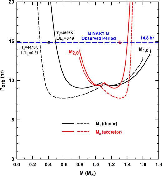
The evolution of representative models for binary B in the Porb–M plane. The black and red curves represent the evolution of the primary (donor) and secondary (accretor), respectively. The solid and dashed curves correspond to two different sets of initial conditions for the progenitor binary. The black and red circles denote the locations of the observationally inferred values of Porb and M for the primary and secondary, respectively. Typical model ages at the current epoch are 2–3Gyr.
According to our proposed scenario, the progenitor primary experiences a phase of rapid mass loss on its Kelvin time while the value of the mass ratio (M2/M1) is ≲1. When the donor’s mass is thus reduced to less than 1 M⊙, it starts to evolve on a nuclear time-scale and the radius of the donor increases (as does Porb). Although this binary evolves above the bifurcation limit (i.e. the donor would eventually become a giant and collapse to become a helium white dwarf), the increase in the mass of the secondary allows it to evolve and fill its Roche lobe before the donor can become a giant. This might lead to a reversal in the direction of mass transfer or a merger might ensue. Regardless of the possible future evolution, we feel confident in stating that the evolution of binary B can be explained without the need to invoke a phase of common envelope evolution. If this is true, then the study of the evolution of binaries A and B can be carried out independently.
10 SUMMARY AND CONCLUSIONS
In this work we have identified a physically bound quadruple system composed of two short-period EBs in an ∼20 au orbit about each other. The doubly eclipsing system was found in Field 7 of the K2 mission, with periods of PA ≃ 3.5949 d and PB ≃ 0.6182 d.
We acquired follow-up ground-based observations including (1) Keck AO images showing that the separation between the two binaries is ≲0.05 arcsec; (2) 20 radial velocity measurements with the NOT-FIES spectrometer that yield single-line RV curves for both binaries; and (3) photometry with small-aperture telescopes (12–14 inch) that yielded nine additional eclipse times, thereby increasing the overall observation interval to nearly 2 yr.
We analyse the photometric and radial velocity data for both binaries all simultaneously to yield many of the binary system parameters. The results are summarized in Table 7.
The ETVs of both binaries show erratic behaviour (binary B) or non-secular trends (binary A), and these are not associated with any LTTEs or physical interactions between the binaries.
We set significant constraints on the outer (i.e. quadruple) orbit using the AO and RV measurements. These indicate that the semimajor axis of the outer orbit is 18 ± 10 au with a likely outer period of 20–40 yr.
The upper limit to the angular separation (from the AO image), the nearly matching γ velocities, and the similar luminosities of the two binaries provide compelling circumstantial evidence for the physical association of the two binaries. By contrast, the detection, at the 3.2σ confidence level, of |$\dot{\gamma }$| for the binary A is important direct evidence that the binaries are physically interacting with one another.
If a few further RV measurements can be made over the next year, the significance of the |$\dot{\gamma }$| detection can be made much stronger. As discussed in the Introduction, there are only a relative handful of double eclipsing quadruples known to be physically bound, and EPIC 219217635 is nearly certain to join their ranks.
Note also that accurate future observations of the complete LTTE orbits of the two binaries will offer all of the benefits that can be obtained from RV measurements of a double-lined spectroscopic binary. And, in addition, because the masses of the two binaries are known relatively well, one will also be able to calculate from the LTTE amplitudes the observed inclination (iout) of the outer orbit.
We would also like to suggest that a few additional RV measurements be made for the next few observing seasons for this system. For outer orbital periods of ∼20 yr, the value of |$\dot{\gamma }_\mathrm{ A}$| would not only be firmed up, but within just a few more years, the curvature of the outer orbit should be detected.
Finally, from our analysis, B binary appears to have its less massive and cooler star evolved well beyond where its main-sequence radius would be, and is filling (or nearly filling) its Roche lobe. We describe a possible evolutionary path to explain this apparent very short period Algol-like red straggler system.
ACKNOWLEDGEMENTS
We are grateful to Jules Halpern for acquiring an initial image of the field at the MDM Observatory. TB acknowledges the financial support of the Hungarian National Research, Development and Innovation Office – NKFIH Grant OTKA K-113117. SA and ABJ acknowledge support by the Danish Council for Independent Research, through a DFF Sapere Aude Starting Grant No. 4181-00487B. AV’s work was supported in part under a contract with the California Institute of Technology (Caltech)/Jet Propulsion Laboratory (JPL) funded by NASA through the Sagan Fellowship Program executed by the NASA Exoplanet Science Institute . MHK, DLC, and T L J acknowledge Allan R. Schmitt for making his light-curve examining software ‘LcTools’ freely available. LN thanks A. Senhadji for technical assistance and the Natural Sciences and Engineering Research Council (Canada) for financial support provided through a Discovery Grant. We also thank Calcul Québec, the Canada Foundation for Innovation (CFI), NanoQuébec, RMGA, and the Fonds de recherche du Québec – Nature et technologies (FRQNT) for computational facilities. The radial velocity spectral observations were made with the Nordic Optical Telescope (NOT), operated by the Nordic Optical Telescope Scientific Association at the Observatorio del Roque de los Muchachos, La Palma, Spain, of the Instituto de Astrofisica de Canarias. The authors are grateful to Davide Gandolfi for time sharing some of his NOT observations between programs. Some of the data presented in this paper were obtained from the Mikulski Archive for Space Telescopes (MAST). STScI is operated by the Association of Universities for Research in Astronomy, Inc., under NASA contract NAS5-26555. Support for MAST for non-HST data is provided by the NASA Office of Space Science via grant NNX09AF08G and by other grants and contracts. A portion of this work was based on observations at the W. M. Keck Observatory granted by the California Institute of Technology. We thank the observers who contributed to the measurements reported here and acknowledge the efforts of the Keck Observatory staff. We extend special thanks to those of Hawaiian ancestry on whose sacred mountain of Mauna Kea we are privileged to be guests. Some results are based on data from the Carlsberg Meridian Catalogue 15 Data Access Service at CAB (INTA-CSIC). This paper includes data collected by the Kepler mission. Funding for the Kepler mission is provided by the NASA Science Missiondirectorate.
Footnotes
In these surveys single A-, F-, or G-type stars are to be counted as ‘systems’.
Most recently Hong et al. (2018) have published an analysis of two double EB candidates in the Large Magellanic Cloud, namely OGLE-LMC-ECL-15674 and OGLE-LMC-ECL-22159. The binaries in the first system exhibit rapid eclipse depth variations, and therefore, probably inclination variations, and one of them also shows rapid apsidal motion. Thus, with high likelihood, this object is also a dynamically interactive, bound quadruple system.
Strictly speaking this is only true for the LTTE. The dynamical contribution to the ETVs would differ due to the different periods of the two inner binaries.
Strictly speaking, this latter quantity was taken into account in a slightly unphysical manner; in particular, it was taken to be an absolutely independent variable, and it was not connected to any variation of the eclipsing period.
After this work was completed, the Gaia DR2 (Lindegren et al. 2018) was released that provides a distance to EPIC 219217635 of 588 ± 17 pc. This is closer than the photometric distance we estimate of 870 ± 100 pc, i.e. based on an approximate extinction of AV ≃ 0.65 ± 0.09. In order for the two distances to be reconciled would require either AV ≃ 1.5 or an unrealistic adjustment of the system MV that we infer from our joint RV and photometric analysis. Another, possibly more likely explanation would be if the finite separation of two binaries on the sky, i.e. ≲0.05 arcsec causes the parallactic distance to be adversely affected (Szabados 1997).
For purposes of discussing the prior evolutionary history of binary B, we have reversed the labels ‘1’ and ‘2’, now referring to the originally more massive star as ‘1’ and vice versa.
This may be an artefact of the uncertainty in the conversion of colours to temperatures.
REFERENCES
,
, in
APPENDIX A: MASS AND TEMPERATURE INFORMATION FROM JOINT PHOTOMETRIC SOLUTION
Author notes
NASA Sagan Fellow.
NSF Astronomy and Astrophysics Postdoctoral Fellow.
