


ABSTRACT
Using a large sample of main sequence stars with 7D measurements supplied by Gaia and SDSS, we study the kinematic properties of the local (within ∼10 kpc from the Sun) stellar halo. We demonstrate that the halo’s velocity ellipsoid evolves strongly with metallicity. At the low-[Fe/H] end, the orbital anisotropy (the amount of motion in the radial direction compared with the tangential one) is mildly radial, with 0.2 <β< 0.4. For stars with [Fe/H] > −1.7, however, we measure extreme values of β∼ 0.9. Across the metallicity range considered, namely−3 < [Fe/H] < −1, the stellar halo’s spin is minimal, at the level of |$20\lt \bar{v}_{\theta }(\mathrm{kms}^{-1}) \lt 30$|. Using a suite of cosmological zoom-in simulations of halo formation, we deduce that the observed acute anisotropy is inconsistent with the continuous accretion of dwarf satellites. Instead, we argue, the stellar debris in the inner halo was deposited in a major accretion event by a satellite with Mvir > 1010M⊙ around the epoch of the Galactic disc formation, between 8 and 11 Gyr ago. The radical halo anisotropy is the result of the dramatic radialization of the massive progenitor’s orbit, amplified by the action of the growing disc.
1 INTRODUCTION
Stars in the Galactic halo formed earlier than those in the disc. However, the epoch of the halo assembly, namely the time at which these stars were deposited into the Milky Way, remains blurry. The onset of star formation in the Galactic disc is bracketed to have happened between ∼8 and ∼11 Gyr ago, based on white dwarf cooling ages (see Oswalt et al. 1996; Leggett, Ruiz & Bergeron 1998; Knox, Hawkins & Hambly 1999; Kilic et al. 2017), isochrone modelling (e.g. Haywood et al. 2013; Martig et al. 2016) and nucleocosmochronology (del Peloso, da Silva & Arany-Prado 2005). The birth times of the halo’s stellar populations can be estimated following the same procedures as for the disc. For example, it has been determined that the halo’s globular clusters range in age from ∼10 to ∼13 Gyr depending on metallicity (see e.g. Hansen et al. 2002, 2007; VandenBerg et al. 2013). Most dwarf spheroidals host stars that are nearly as old as the Universe itself (see Tolstoy, Hill & Tosi 2009), while many ultra-faint dwarfs appear to have formed the bulk of their stellar populations only slightly less than a Hubble time ago (see e.g. Belokurov et al. 2007; Brown et al. 2014). In the field, the halo stars have ages in the range of 10–12Gyr (Jofré & Weiss 2011; Kilic et al. 2012; Kalirai 2012).
The first attempt to decipher the history of the formation of the Galactic disc and the stellar halo can be found in Eggen, Lynden-Bell & Sandage (1962). Based on the strong apparent correlation between the metallicity of stars in the Solar neighbourhood and the eccentricity of their orbits, the authors concluded that the metal-deficient stars formed first in an approximately spherical configuration. This original gas cloud then collapsed in a nearly instantaneous fashion, giving birth to the subsequent generations of stars. The contraction of the Galaxy not only yielded a population of younger stars on nearly circular orbits, but also profoundly affected the orbital shapes of the old stellar halo. As Eggen et al. (1962) demonstrate, driven by the collapse, the orbits of the halo stars ought to become highly eccentric, thus explaining the chemo-kinematic properties of their stellar sample. Later studies (see e.g. Norris, Bessell & Pickles 1985; Beers & Sommer-Larsen 1995; Carney et al. 1996; Chiba & Yoshii 1998) revealed that the claimed correlation between the eccentricity and metallicity might have been caused by a selection bias affecting the data set considered by Eggen et al. (1962). Notwithstanding the concerns pertaining to the observational properties of their data, the theoretical insights into the dynamics of the young Galaxy gained by Eggen et al. (1962) are as illuminating today as they were 50 years ago.
Whilst the hypothesis of strict ordering of the orbital properties with metallicity in the stellar halo is not supported by the data, it is undeniable that a large fraction of the halo stars are metal-poor and do move on eccentric orbits. In spherical polar coordinates, the shape of the stellar halo’s velocity ellipsoid can be characterized by one number, the anisotropy parameter: |$\beta =1-[({\sigma_{\theta }^2+\sigma_{\phi }^2})/{2\sigma_r^2}]$|, where β = −∞ for circular orbits and β= 1 for radial ones. In the Solar neighbourhood, the halo’s velocity ellipsoid is evidently radially biased. For example, Chiba & Yoshii (1998) obtained β = 0.52 for a small sample of local halo red giants and RR Lyrae observed by the Hipparcos space mission. Using the SDSS Stripe 82 proper motions, and thus going deeper, Smith et al. (2009a) measuredβ= 0.69 using ∼2000 nearby subdwarfs. Combining the SDSS observations with the digitized photographic plate measurements, Bond et al. (2010) increased the stellar halo sample further and derived β= 0.67. For slightly larger volumes probed with more luminous tracers, similar values of β ∼ 0.5 were obtained (see e.g. Deason et al. 2012; Kafle et al. 2012). Unfortunately, beyond 15–20 kpc from the Sun, the behaviour of the anisotropy parameter is yet to be robustly determined. While there have been several attempts to tease β out of the line-of-sight velocity measurements alone (see e.g. Sirko et al. 2004; Williams & Evans 2015), Hattori et al. (2017) have shown that these claims need to be taken with a pinch of salt. Curiously, the only distant stellar halo anisotropy estimate that actually relies on the proper motion measurements (with theHubble Space Telescope) reports a dramatic drop to β ∼ 0 at ∼20 kpc (see Deason et al. 2013b; Cunningham et al. 2016), albeit based on a very small number of stars.
Theoretically, the behaviour of the orbital anisotropy in the dark halo has been scrutinized thoroughly. As demonstrated by Navarro et al. (2010), in the Aquarius suite of simulations, β starts as nearly isotropic in the centre of the galaxy, reaches β∼ 0.2 around the solar radius and keeps increasing to β∼ 0.5 at >100 kpc, before decreasing again to zero around the virial radius. The picture becomes somewhat muddled when the effects of baryons are included. According to Debattista et al. (2008), halo contraction as a result of baryonic condensation may make the dark matter (DM) haloes slightly more radially anisotropic, but overall the changes are small and the β trends with Galacto-centric distance are preserved. On the other hand, when the Aquarius haloes are re-simulated with added gas physics and star formation, only some galaxies retain their DM-only anisotropy trends, while in others the β profile flattens and stays constant with β ∼ 0.2 throughout the galaxy (see Tissera et al. 2010). Even though, crudely, the physics of the formation and evolution of the dark and the stellar haloes are the same, their redshift z= 0 properties may be drastically different owing to the highly stochastic nature of the stellar halo accretion (see e.g. Cooper et al. 2010). Indeed, in numerical simulations of stellar halo formation, the anisotropy behaviour differs markedly from that of the DM one. Already in the central parts of the Galaxy, β quickly reaches ∼0.5 and rises further to β ∼ 0.8 at 100 kpc, showing a much smoother monotonic behaviour all the way to the virial radius (see e.g. Abadi, Navarro & Steinmetz 2006; Sales et al. 2007; Rashkov et al. 2013; Loebman et al. 2018).
In this paper, we explore the behaviour of the stellar halo velocity ellipsoid as a function of metallicity and distance above the Galactic plane. Our sample is based on the SDSS DR9 spectroscopic data set and consists of main sequence stars with distances between <1 and ∼10 kpc from the Sun. The stars included in the analysis overlap widely with selections considered by several groups previously (see Smith et al. 2009a; Bond et al. 2010; Loebman et al. 2014; Evans et al. 2016). However, thanks to the Gaia DR1, the proper motions of these stars are now measured with an improved accuracy. Section 2 gives the details of the stellar sample under consideration, as well as the model used to characterize the stellar halo behaviour. The implications of our findings and a comparison with numerical simulations of the stellar halo formation are presented in Section3.
2 DATA AND MODELLING
2.1 Main sequence stars in SDSS-Gaia
We selectedmain sequence stars from the SDSS DR9 spectroscopic sample (Ahn et al. 2012) using the following cuts: |b| > 10°, Ag < 0.5 mag, σRV < 50 km s−1, S/N>10, 3.5 < log (g) < 5, 0.2 < g − r < 0.8, 0.2 < g − i < 2, 4500 K<Teff < 8000 K and 15 < r < 19.5. All magnitudes were de-reddened using dust maps from Schlegel, Finkbeiner & Davis (1998). A total of 192536 stars survived the above cuts. We estimated the stars’ distances using equations (A2), (A3) and (A7) in Ivezić et al. (2008). The proper motions were obtained using a crossmatch between the SDSS and Gaia catalogues. The SDSS catalogue has been astrometrically recalibrated using the GaiaSource positions in order to correct both small- and large-scale systematic astrometric errors. The resulting SDSS-Gaia proper motion catalogue covers the entirety of the high-latitude SDSS sky with baselines between 6 and 18 yr. Deason et al. (2017) and de Boer, Belokurov & Koposov (2018) assessed the quality of the catalogue and demonstrated that it suffers little from systematic biases and clearly outperforms the SDSS-Gaia catalogues relying on the original SDSS astrometric solution. For each star, given the position on the sky and the distance, the proper motion and the line-of-sight velocity were converted to Galacto-centric Cartesian velocity components assuming the local standard of rest of 235 km s−1 and the components of the solar peculiar motion presented in Coşkunoǧlu et al. (2011). The uncertainties in distance, line-of-sight velocity and proper motion were propagated using Monte Carlo (MC) sampling to obtain the final uncertainties on the velocity components in spherical polar coordinates. Accordingly, for each star, its Galacto-centric coordinates and velocity components are the median values of the resulting MC distribution, and the associated ‘error-bars’ are the median absolute deviation values scaled up by a factor of 1.48. To removethe obvious outliers we culled |$0.1\hbox{ per cent}$| of stars with excessively high speeds. Note that the (magnitude-independent and metallicity-independent) proper motion uncertainties were estimated using equation (2) provided in Deason et al. (2017) (for further discussion, see de Boer et al. 2018). Furthermore, neither the selection procedure above nor the SDSS spectroscopic targeting scheme (with the exception of the K-giant sample not used here) includes restrictions based on the stellar kinematics. Therefore, we believe that the sample considered here is kinematically unbiased. Fig. 1 shows the density distribution of stars in our sample. A strong spatial bias due to the SDSS spectroscopic selection is clearly visible in the left panel, where stars can be seen reaching 3 <R (kpc) <23 and |z| < 9 kpc. The right panel gives the distribution of the stellar metallicity as a function of the Galactic height. A metal-rich, namely [Fe/H]∼0, component corresponding to the Galactic disc is apparent at |z| < 1 kpc. Curiously, a low-height density enhancement is also discernible at low metallicities, namely at [Fe/H] <−1.
![Galacto-centric view of the SDSS-Gaia sample. Left: Logarithm of the stellar density in cylindrical R, z-coordinates. Right: Logarithm of the stellar density in the plane of [Fe/H] and Galactic height z. The horizontal dotted lines give the range of heights considered in the velocity ellipsoid analysis.](https://oup.silverchair-cdn.com/oup/backfile/Content_public/Journal/mnras/478/1/10.1093_mnras_sty982/2/m_sty982fig1.jpeg?Expires=1750237004&Signature=XbzTpovLYXJthKgZTP~YDtenkNxRNx1WGRJNC1fcSPWvL91CikuVCTnrykE3PISir~b8wPhN7rSxoUl4jRK-cpgQOq9VvfUlsBoEBfVumkAO-v4JCizgOnRdsKN8qWzQXsBjBerJQOyAxsECW3YPD-8nWEg0v4991fu4pVCuw4V0qAWC-x7zyLKx1Ze15COjUfj1pk2zpRPAdn9o5k6gvlD1bjNPeXt9C7kAz7UZeK1DdWLvYuHl4WNQ2wkZbDLN5kcl6LqwGRFmBy61Tg0c68TRAw8Bo5W0GlLf2Gfx0IuQ87XpOIG8irxclDtNpwgApMSXSwY10r5zpTesaFjYMg__&Key-Pair-Id=APKAIE5G5CRDK6RD3PGA)
Galacto-centric view of the SDSS-Gaia sample. Left: Logarithm of the stellar density in cylindrical R, z-coordinates. Right: Logarithm of the stellar density in the plane of [Fe/H] and Galactic height z. The horizontal dotted lines give the range of heights considered in the velocity ellipsoid analysis.
In addition to the survey-induced systematics, there may exist other observational biases that could affect the measurements reported in this work. For example, a large and non-constant fraction of unresolved binary objects amongst the stars considered here could influence the kinematics in the following way. The stellar distances, as predicted by the equations in Ivezić et al. (2008), are appropriate for single stars. However, if instead a star is an unresolved binary, it will appear brighter at a fixed colour as compared with the fiducial relation. This will in turn lead to an underestimated photometric distance and therefore to an underestimated tangential velocity. Despite the fact that all stars considered here have spectra, most of the potential binaries would remain undetected. This is because the fraction of stars with a clear spectroscopic binary signature (i.e. doubling of all absorption lines) is expected to be small, owing to (i) the low spectral resolution of the SDSS, and (ii) the fact that the binary star period distribution peaks at 105 d (see Raghavan et al. 2010), thus yielding minuscule line shifts. To understand the possible impact of the binarity on our results, we carried out the following simple test. We generated a mock stellar sample corresponding to an old (12 Gyr) metal-poor ([Fe/H] = −1) stellar population. The masses of the stars were drawn from the Chabrier initial mass function, their distances from a ρ ∝ r−2 radial density distribution (from 0.1 to 100 kpc) and their velocities from a Gaussian with a constant velocity dispersion of 100 km s−1. Assuming binary fractions of 0, 0.5 and 0.9 and a uniform mass ratio distribution (see Raghavan et al. 2010), we calculated the impact of the binaries on the measured tangential velocity dispersions. Reassuringly, for the substantial 50 per cent binary fraction, only a 10 per cent lower velocity dispersion is registered. For an unrealistically high 90 per cent binary fraction, the tangential velocity dispersion would be underestimated by 20 per cent. Accordingly, we believe that our velocity dispersion measurements (see below) are largely insensitive to the presence of unresolved binary stars in the sample.
2.2 7D view of the local stellar halo
Fig. 2 shows the evolution of the azimuthal, vθ, and the radial, vr, velocity components of the stellar sample defined in the previous subsection as a function of metallicity, [Fe/H], and height above the Galactic disc, |z|. As our focus is on the Galactic halo, we chose to project stellar velocities onto spherical polars. This is motivated by a number of recent studies demonstrating that the halo’s second velocity moment tensor is nearly spherically aligned (e.g. Smith, Wyn Evans & An 2009b; Bond et al. 2010; Evans et al. 2016; Posti et al. 2017). Note that we use the spherical polar convention in which θ is the azimuthal angle andϕ is the polar angle. The interested reader may wish to compare the kinematic properties of the halo presented below with those derived in cylindrical polar coordinates in Myeong et al. (2018b). In Fig. 2, the metallicity of the stars considered increases from left to right and the Galactic height increases from top to bottom. In the distributions of the stars closest to the Galactic plane (top row), two components with different kinematic properties are clearly discernible. The (thick) disc has a negligible mean radial velocity, |$\bar{v}_r\sim 0$| km s−1, and a significant rotation, |$\bar{v}_{\theta }\sim 200$| km s−1. Much hotter in terms of its velocity dispersion, especially in the r direction, is the stellar halo, whose rotation |$\bar{v}_{\theta }$| is extremely weak. As the stars become progressively more metal-poor (from right to left), the rotating component fades, and disappears completely when observed at greater heights (middle and bottom rows). Note that, as shown in the top left corner of each panel, the velocity error changes strongly as a function of the Galactic |z| and for fixed |z| is approximately constant across the entire metallicity range. The evolution of the error with height is driven by the dependence of the tangential velocity on distance and the distance error on the photometric uncertainty.
![Behaviour of the velocity components in spherical polar coordinates, namely radial vr and azimuthal vθ, for stars in the SDSS-Gaia main sequence sample. The data set is divided into metallicity bins, [Fe/H], increasing from left to right and Galactic height bins, |z|, increasing from top to bottom. The size of the median velocity error for each subset is shown in the top left corner of each panel, and the total number of stars in that bin can be found in the top right corner. The pixel size is 20 × 20 km s−1. The distribution of the metal-rich stars near the Galactic plane (top right corner of the panel grid) displays two distinct populations: a cold rotating one (the thick disc) and a barely rotating, markedly radially anisotropic one (the stellar halo). Moving from top to bottom, (i.e. to greater heights), the Galactic disc contribution quickly diminishes. From right to left (i.e. from metal-rich to metal-poor), the stellar halo’s velocity ellipsoid evolves from strongly radial to significantly more isotropic.](https://oup.silverchair-cdn.com/oup/backfile/Content_public/Journal/mnras/478/1/10.1093_mnras_sty982/2/m_sty982fig2.jpeg?Expires=1750237004&Signature=pUfC1nVRjuCeVfYrb4cohNQx~YYLAQudUBLowDSvYQ7lwEfz4pBio3vrLJqEoeS3HH~hPfrTGurCwtlO3Vt~OXG5O2C7kurgmkFcyYtYpZcoBERfMBqYUExW992YNBcx~93EpHKtPG6DOi0awizgRaiF8S~vBnWQ3DF3Rc1Fj4f5TXJ8oT0oSfTOoN1Q~28oqIojoILe6Ed~xIACA3B7H28DwUmSMvFnsngF24hk-5271DqTLfylFsXG05~kuEjHf2-RWP0O7gEGPuazaVVtbwl3WDRjsHR2TUXuQg6vovTRTpx74vz-MBTF-i-EuhCx2YM4F9t0qcUV82F0Licgrw__&Key-Pair-Id=APKAIE5G5CRDK6RD3PGA)
Behaviour of the velocity components in spherical polar coordinates, namely radial vr and azimuthal vθ, for stars in the SDSS-Gaia main sequence sample. The data set is divided into metallicity bins, [Fe/H], increasing from left to right and Galactic height bins, |z|, increasing from top to bottom. The size of the median velocity error for each subset is shown in the top left corner of each panel, and the total number of stars in that bin can be found in the top right corner. The pixel size is 20 × 20 km s−1. The distribution of the metal-rich stars near the Galactic plane (top right corner of the panel grid) displays two distinct populations: a cold rotating one (the thick disc) and a barely rotating, markedly radially anisotropic one (the stellar halo). Moving from top to bottom, (i.e. to greater heights), the Galactic disc contribution quickly diminishes. From right to left (i.e. from metal-rich to metal-poor), the stellar halo’s velocity ellipsoid evolves from strongly radial to significantly more isotropic.
The most notable feature of Fig. 2 is the appearance of the stellar halo velocity ellipsoid. The halo’s distribution is demonstrated to be stretched dramatically in the radial direction for stars in the high-metallicity range, namely for −1.7 <[Fe/H] < −1. However, at lower metallicity, it evolves rapidly to an almost spherical shape. In order to track the behaviour of the stellar halo’s velocity ellipsoid, we model the stellar distributions shown in Fig. 2 with a mixture of multi-variate Gaussians using the Extreme Deconvolution algorithm described in Bovy, Hogg & Roweis (2011). Given the number of stars and the complexity of the overall velocity distribution, which evolves quickly as a function of metallicity and Galactic |z|, we use different numbers of Gaussian components for each subsample. The two lowest-metallicity bins and the highest-|z| bin are always modelled with one 3D Gaussian (according to the number of the velocity dimensions in spherical polars). For all other subsets, in a 3× 2 array in the top right corner of Fig. 2 we attempt to fit three 3D Gaussian components. However, if the resulting component contains less than 3 per cent of the total number of stars in a given subsample we do not report its properties. The uncertainties of the model parameters are estimated using the bootstrap method.
The results of the multi-Gaussian decomposition of the velocity distributions are shown in Fig. 3. Here, the significant (i.e. containing |$\gt 3\hbox { per cent}$| of the total number of stars) model components are over-plotted on top of the model residuals for each subset in the metallicity and |z| space.White solid lines give the projection of the disc’s velocity ellipsoid, and black solid lines show the main halo component. In four cases, two in the top and two in the middle row, a third halo-like Gaussian (white dashed line) was required to describe the data: in these cases its contribution varied between 5 and 15 per cent of the total number of stars in the bin. As displayed in the figure, the overall quality of the fits is good, changing from excellent at the metal-poor end to satisfactory at the metal-rich extreme. Most metal-rich distributions show clear over-densities of stars with high radial velocities, both positive and negative. These high vr ‘lobes’ are most visible in the two right columns of the figure. In addition, some smaller-amplitude residuals are also discernible, for example for the stars closest to the disc, in the most metal-rich bin (top right corner of the grid) and for example at vθ ∼ 150 km s−1 for the stars with lowest metallicity (top left corner and adjacent).
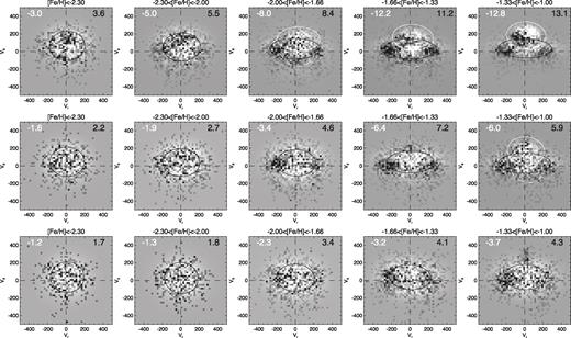
Residuals (data model) of the fit to the distributions shown in Fig. 2. Dark (white) corresponds to an excess (depletion) of stars in the data compared with the model. The number of stars per pixel contributing to the highest positive (negative) residuals are shown in the right (left) corner of each panel. The Gaussian components used to describe the data are also shown: solid white for the disc, solid black for the main halo, and white dashed for the additional halo-like component. Note a clear pattern of excess–depletion–excess along the radially stretched halo component on the right-hand side of the grid. The appearance of the metal-rich halo residuals clearly indicates that the observed velocity distribution is strongly non-Gaussian. Also note small but discernible disc-like residuals in the top-left corner of the grid (corresponding to the metal-poor stars near the Galactic plane).
Fig. 4 summarizes the evolution of the individual velocity disperions σr, σθ and σϕ (left) and the resulting orbital anisotropy (middle) of the stellar halo as a function of metallicity for three Galactic height ranges. Also shown is the behaviour of the rotation |$\bar{v}_{\theta }$| of the main halo (right). As hinted at in Figs 2 and 3, σr, σθ, σϕ and β are all a strong function of the stellar metallicity. However, this dependence does not appear to be gradual. Instead, a sharp transition in the properties of the stellar halo’s ellipsoid can be seen at [Fe/H]∼ −1.7. For more metal-rich halo stars, the anisotropy is acutely radial, with β reaching values of 0.9! However, the halo traced by the most metal-poor stars is almost isotropic, with 0.2 <β < 0.4. Note also that while a visual inspection of Fig. 2 registers a noticeable swelling of the velocity ellipsoid with Galactic |z|, this effect is mostly the result of an increase in the velocity error (as shown in the top left corner of each panel). The final, deconvolved velocity dispersions take each star’s velocity uncertainty into account and show little change in the velocity ellipsoid shape as a function of |z| (see Fig. 4). In terms of the halo rotation, interesting yet more subtle trends are apparent. Stars more metal-rich than [Fe/H]∼ −1.7 show a prograde spin |$20 \lt \bar{v}_{\theta } (\mathrm{kms}^{-1}) \lt 30$| irrespective of the height above the Galactic plane. The rotation of the metal-poorer stars decreases as a function of |z|, from ∼50 km s−1 near the plane to <15 km s−1 at 5 < |z|(kpc) < 9. Overall, based on the analysis presented here, the stellar halo appears to be describable, albeit crudely, with a superposition of two populations with rather distinct properties.
![Derived properties of the velocity ellipsoid of the main stellar halo component as a function of metallicity for three distances from the Galactic plane (indicated by colour). Left: Velocity dispersion along each of the three dimensions. Note that for [Fe/H] > −1.7, the radial velocity dispersion (σr, solid lines) is approximately three times larger than those in the θ (dotted) and ϕ (dashed) dimensions. At the metal-poor end, the three velocity dispersions come much closer to each other. Middle: Velocity anisotropyβ of the stellar halo. Note a sharp change in β from nearly isotropic at low metallicity to extremely radial for the chemically enriched stars. Right: Amplitude of rotation $\bar{v}_{\theta }$. The spin of the metal-rich stellar halo subpopulation $20\lt \bar{v}_\theta ($kms−1) < 30 is independent of the Galactic height. The amount of rotation in the metal-poor stars appears to evolve with |z|. However, as explained in the main text, this is largely the result of low but non-negligible disc contamination and an oversimplified model (one Gaussian component for the two most metal-poor subsamples).](https://oup.silverchair-cdn.com/oup/backfile/Content_public/Journal/mnras/478/1/10.1093_mnras_sty982/2/m_sty982fig4.jpeg?Expires=1750237004&Signature=kgssDsfW2-XempRKbcf4rpFnpDyTk~DYJX2sJsOIQ3j-fdt37mSTkp1DsU1-0Tl-wV0hIv-oeaXdCJW6Ofyc0SM9vrmDPpXkdaQw~S8dBDUwrd5wVg~s0WdJfZElX8ZmWrp3TgStznAO2yMqLX~Z7bt7xc3r5SOT~wPugcZewhcq1FAP2XOKHYzAsFPhOPb5wwSjukKp43hRKDCBc3XtTOeGfcwP6-gsTVE8e0Jp17NoYQH7V7mr4STXYEyfoL9gTwfG46dvubDimssBQJu95vp1umMvSucqzNA8bD8gGxAEKZy-S~Ycu-FfSLVvoNt-nBV4DtlGJf4cVhAmk6l7Og__&Key-Pair-Id=APKAIE5G5CRDK6RD3PGA)
Derived properties of the velocity ellipsoid of the main stellar halo component as a function of metallicity for three distances from the Galactic plane (indicated by colour). Left: Velocity dispersion along each of the three dimensions. Note that for [Fe/H] > −1.7, the radial velocity dispersion (σr, solid lines) is approximately three times larger than those in the θ (dotted) and ϕ (dashed) dimensions. At the metal-poor end, the three velocity dispersions come much closer to each other. Middle: Velocity anisotropyβ of the stellar halo. Note a sharp change in β from nearly isotropic at low metallicity to extremely radial for the chemically enriched stars. Right: Amplitude of rotation |$\bar{v}_{\theta }$|. The spin of the metal-rich stellar halo subpopulation |$20\lt \bar{v}_\theta ($|kms−1) < 30 is independent of the Galactic height. The amount of rotation in the metal-poor stars appears to evolve with |z|. However, as explained in the main text, this is largely the result of low but non-negligible disc contamination and an oversimplified model (one Gaussian component for the two most metal-poor subsamples).
Ours is not the first claim for the existence of (at least) two distinct components of the stellar halo (see e.g. Chiba & Beers 2000; Carollo et al. 2010). If the kinematic properties are measured locally, then it is possible to estimate the 3D volume density behaviour of each of the halo components (May & Binney 1986; Sommer-Larsen & Zhen 1990). Based on the studies above, the more metal-rich halo component was inferred to possess a flatter (with respect to the Galactic vertical direction) distribution of stars. Note that a similar argument based on the virial theorem is presented in Myeong et al. (2018b), who analyse a data set nearly identical to that presented here and estimate the amount of flattening in each of the two halo components. Thus, the recently revealed evolution of the shape of the stellar halo with Galactocentric distance (see e.g. Xue et al. 2015; Das, Williams & Binney 2016; Iorio et al. 2017) could be interpreted as a change in the contribution from each component. Given that our stellar sample extends as far as 10 kpc above the disc plane, it may be possible to track the differences in the density distribution in the metal-rich and metal-poor subpopulations. Unfortunately, this calculation is not straightforward to carry out in view of the strong (metallicity- and magnitude-dependent) selection biases of the SDSS spectroscopic survey. At the zeroth order – and not accounting for any selection biases – we do not record any significant changes in the fraction of stars locked in the more metal-rich component (i.e. with −1.66 <[Fe/H] < −1) with Galactic height: it remains at a level of ∼66 per cent across all |z| studied.
3 DISCUSSION AND CONCLUSIONS
This paper uses the SDSS-Gaia proper motions, and thus our data set is nearly identical to that of Myeong et al. (2018a,b). As shown by Deason et al. (2017) and de Boer et al. (2018), both random and systematic proper motion errors in the SDSS-Gaia catalogue are minimized compared with most previously available catalogues of similar depth. Instead of attempting to identify a subsample of halo stars, we model the entirety of the data with a mixture of multi-variate Gaussians. This allows us to avoid any obvious selection biases and to extract a set of robust measurements of the stellar halo velocity ellipsoid. As seen by SDSS and Gaia, the properties of the local stellar halo are remarkable. We show that the shape of the halo’s velocity ellipsoid is a strong function of stellar metallicity, where the more metal-rich portion of the halo, namely that with −1.7 <[Fe/H] < −1, exhibits extreme radial anisotropy, namely 0.8 <β < 0.9 (see Fig. 4). Co-existing with this highly eccentric and relatively metal-rich component is its metal-poor counterpart with −3 <[Fe/H] < −1.7 and β ∼ 0.3. The velocity ellipsoid evolves rapidly from mildly radial to highly radial over a very short metallicity range, changing β by ∼0.6 over 0.3 dex. The two stellar halo components also display slightly different rotational properties. The more metal-enriched stars show a mild prograde spin of ∼25 km s−1 irrespective of Galactic height z. The spin of the metal-poor halo evolves from ∼50 km s−1 at 1 < |z|(kpc) < 3 to ∼20 km s−1 at 5 < |z|(kpc) < 9. Note, however, that while the stellar halo’s properties change sharply at [Fe/H]∼ −1.7, we do not claim that the more isotropic component does not exist at higher metallicities [Fe/H] > −1.7; it is just much weaker (see the white dashed contours in Fig. 3).
Before we discuss the implications of the measurements presented above for the genesis of the stellar halo, let us briefly compare the properties of the velocity ellipsoid deduced here with those in the literature. Most of the recently published halo anisotropy values are close to β < 0.7 (e.g. Smith et al. 2009a; Bond et al. 2010; Posti et al. 2017), significantly lower than the β ∼ 0.9 reported here. We believe, however, that there is no obvious disagreement as previous estimates combine stars across the entire metallicity range and therefore represent an average over the [Fe/H]-dependent values we measure. In terms of the halo spin, the amount of prograde rotation at high |z| is consistent with the majority of both past and recent studies of the stellar halo (see e.g. Chiba & Beers 2000; Deason et al. 2017).
What could be the cause of the dramatic radial anisotropy registered at high metallicity and what is the nature of the striking bimodality in the behaviour of the stellar halo presented in the previous section? The two currently available theories for the formation of the stellar halo in the vicinity of the Galactic plane invoke (i) accretion and disruption of multiple satellites, and (ii) in situ formation of a puffed-up rotating halo via the disc heating. However, it is hard to fathom how the observed extremely radial velocity anisotropy could be reconciled with either of these scenarios without any modification. We are not aware of any in situ halo model where (i) the resulting halo possesses highly radial anisotropy and (ii) the rotation signal would be as low as measured here, namely ∼25 km s−1 (as judged by the more metal-rich subset of our halo stars). Equally difficult to imagine is the idea that a prolonged accretion of multiple low-mass Galactic fragments can yield such high values of β. Given that the accreted satellites should show a diversity of orbital properties, it is more natural to expect a much more isotropic velocity ellipsoid, perhaps similar to what we observe at low metallicities, but wildly different from that of the metal-enriched stars, namely the bulk of the stellar halo near the Sun.
Recently, several arguments have been put forward to support the idea of the halo formation through a single dominant accretion event some ∼10 Gyr ago (see e.g. Deason et al. 2013a; Belokurov et al. 2017). In this scenario, one massive merger provides the lion’s share of the halo stars within ∼30 kpc of the Galactic centre. At this characteristic radius (see e.g. Deason, Belokurov & Evans 2011; Sesar, Jurić & Ivezić 2011), the properties of the stellar halo appear to change dramatically, leading Deason et al. (2013a) to argue that this transition scale may correspond to the last apo-centre of the halo’s progenitor before disruption. The hypothesis in which a large portion of the inner Galaxy’s halo is dominated by the stellar debris from a massive satellite is consistent with the abundance patterns of light elements in the halo. The absence of prominent sequences corresponding to contributions from low-mass systems as well as the iron abundance at the characteristic ‘knee’ of the stellar halo’s [α/Fe] distribution (see e.g. Venn et al. 2004; Tolstoy et al. 2009; de Boer et al. 2014) could all be explained with the (early) accretion of a massive progenitor. This interpretation is supported by the study of Amorisco (2017), who has built a large library of toy models of idealized merger events in an attempt to provide an atlas of the halo properties corresponding to different accretion histories. The models confirm the conclusions of Deason et al. (2013a) that massive satellites are able to sink deeper in the potential well of the Galaxy owing to dynamical friction, thus dominating the inner halo of the Galaxy. In addition, Amorisco (2017) showed that the evolution of the orbital properties of the in-falling dwarfs depends strongly on their mass: the low-mass systems might experience some mild orbital circularization, while the orbits of the more massive systems tend to radialize rather strongly. Therefore, for high mass-ratio events, as a result of the pronounced orbital radialization, the resulting stellar halo possesses negligible spin at redshift z = 0. This is in excellent agreement with the most recent measurement by Deason et al. (2017) and with the results presented here.
We seek to verify the above hypothesis using a suite of numerical simulations that improve on those discussed in the literature so far (such as those by Bullock & Johnston 2005 and Amorisco 2017). We consider 10 cosmological zoom-in simulations of the formation of the stellar halo around galaxy hosts with masses similar to that of the Milky Way. These simulations are described in detail in Jethwa, Erkal & Belokurov (2018) and Belokurov et al. (2017) and are run with the N-body part of gadget-3, which is similar to gadget-2 (Springel 2005). Our stellar halo realizations (based on tagging the most bound particles in satellites; De Lucia & Helmi 2008; Bailin et al. 2014) are similar to those presented in Bullock & Johnston (2005) and Amorisco (2017) in the way that they do not attempt to model the gas dynamics and the feedback effects. They contain, however, some of the salient features necessary to understand the stellar halo emergence, such as the mass function and the accretion time of the satellite galaxies, as well as the effect of the Galactic disc on the properties of the DM halo and the in-falling subhaloes. In our suite, all 10 simulations are run twice, once without a disc, and once including the effects of a disc. The disc is represented by a parametric Miyamoto–Nagai potential (see Miyamoto & Nagai 1975), whose mass is grown adiabatically from redshift z = 3 to z= 1, or, in lookback time, from 11 to 8 Gyr ago. Fig. 5 shows the orbital properties of the stellar debris as observed today in the vicinity of the Sun as a function of the accretion time for three progenitor mass ranges. Clearly, the simulated redshift z = 0 halo contains a mixture of debris with a wide range of orbital properties. However, a trend is discernible in which the most massive satellites (red line) contribute stars on strongly radial orbits. Moreover, the highest anisotropy values β ∼ 0.8 are recorded for the stellar debris deposited during the phase of the disc assembly (greyregion).
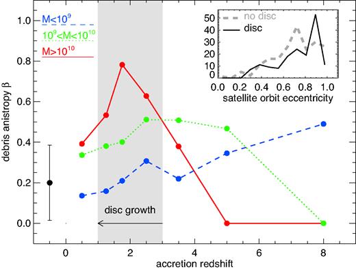
Velocity anisotropy of the stellar debris in the solar neighbourhood (4 <R(kpc) < 25, roughly matching the range probed by the data) as a function of the progenitor’s accretion redshift for three subhalo mass ranges. Each data point gives the median value across the suite of 10 simulations. The highest radial anisotropy (for the considered range of Galactocentric radii) is attained by the debris from the most massive progenitors (Mvir > 1010M⊙, red line) accreted between z = 1 and z= 3, namely during the disc growth phase (corresponding to 8 to 11 Gyr of lookback time, grey shaded region). The error-bar on the left-hand side gives an estimate of the typical scatter in an individual (redshift, mass) bin. In the inset, the black solid (grey dashed) line shows the distribution of the final orbital eccentricity for the satellites with Mvir > 1010M⊙ and accretion redshift 1 < z < 3 with (without) the baryonic disc included. Even without the action of the disc, the distribution of eccentricities has a peak at e> 0.7. The presence of the disc enhances the orbital radialization, pushing the peak of the distribution to e > 0.9.
Such synchronicity between the epoch of the disc growth and the occurrence of massive accretion events is not surprising. Before subhaloes with virial masses Mvir > 1010M⊙ can be accreted and destroyed they need to have time to grow. For example, from an extrapolation of the median halo formation time as shown in figs 4 and 5 of Giocoli et al. (2007), the most massive Milky Way satellites would not have been assembled before redshift z ∼ 2. However, there are additional factors that may explain the coincidence of the disc development and the peak in the β profile in Fig. 5. The inset in the top-right corner of the figure shows the distribution of the orbital eccentricities of the subhaloes with Mvir > 1010M⊙ accreted at 1 < z < 3. Even without the action of the baryonic disc (dashed grey line), the eccentricity distribution appears to peak at e > 0.7, in agreement with the findings of Amorisco (2017). Note, however, that the peak of the distribution is pushed to even higher values, namely e> 0.9, when the disc is included (solid black line). Thus, we conclude that the satellite radialization at the high-mass end is enhanced by the presence of the growing disc, acting to promote extreme values of the velocity anisotropy of the inner stellar halo as observed today.
Using the intuition informed by the numerical experiments described above, let us return to the view of the stellar halo given in Figs 2 and 3. The radically radial component of the nearby stellar halo is also the one that contains the most metal-rich halo stars, in agreement with the mass–metallicity relationship observed in dwarf galaxies (Kirby et al. 2013). Note, however, that in the (vr, vθ) plane the density distribution of this sausage-like population is not exactly Gaussian, as manifested by a pronounced excess of stars with high positive/negative radial velocity (see Fig. 3). We believe, though, that the black–white–black pattern of the residual distribution on the right-hand side of the figure can be equally well explained by the lack of stars with low radial speeds. This interpretation may be more appropriate if the Sun is located somewhere in the middle of a giant cloud of stars on highly radial orbits (with their peri-centres at small Galactic radii and the apo-centres not far from the break radius at ∼30 kpc). Because we are limited by the available data, our view of the halo lacks stars near the turning points – apos and peris – where the radial motion is the slowest. This explanation echoes the discussion presented in Meza et al. (2005) (see also Navarro et al. 2011), where the locally sampled velocity distribution of a high-energy accretion event appears sharply double-horned. Most importantly, given that as a result of the selection effect described above the velocity distribution is noticeably non-Gaussian, the (already high) anisotropy value for the metal-rich component may actually be an underestimate.
Notwithstanding the strong radialization of the progenitor’s orbit, it is unlikely that it would lose all of its angular momentum. In this regard, the low-amplitude yet clearly detectable spin of the metal-rich halo component could simply be the relic of the orbital angular momentum of the parent dwarf before dissolution. This interpretation also agrees with the observed constancy of the rotation amplitude of the metal-rich halo with the height above the Galactic plane. Given the range of vertical distances probed here, any significant change in the amount of rotation would imply that the scale-height of the halo component considered is not dissimilar to that of the thick disc. This can be contrasted with the behaviour of the metal-poor halo subpopulation. The amount of rotation at the metal-poor end is inversely proportional to the height above the plane. The strongest signal of >50 km s−1 is detected near the Galactic plane. As the two top-left panels of Fig. 3 demonstrate, the single-Gaussian model produces noticeable residuals at vθ ∼ 150 km s−1. Given the appearance of the model residuals for the lowest-height subsample (top left panels), we conjecture that the halo spin is probably an overestimate owing to the presence of a non-negligible number of non-halo stars in apparent prograde rotation. Interestingly, at metallicities [Fe/H] <−1.3 we recover a small but statistically significant positive radial velocity for stars contributing to this disc-like population. This is consistent with the analysis of Myeong et al. (2018b), who also show that the excess of rotating metal-poor stars with 0 <vr(kms−1) < 20 is a strong function of Galacto-centric radius. Thus, it is unlikely that this signal is provided by a (thick) disc alone. Instead we conjecture that this could plausibly be a combination of an extremely metal-poor disc and stars trapped in a resonance with a bar, a feature known as the Hercules stream (see Dehnen 2000; Antoja et al. 2014; Hunt et al. 2018). At larger distances from the Galactic plane, the contribution of the disc at the metal-poor end sharply subsides and the velocity distribution can be adequately described with a single Gaussian, yielding spin values comparable to (or sometimes slightly lower than) those observed at the metal-rich end.
An alternative explanation of the strong radial anisotropy observed in the stellar halo may be provided by the ideas of Eggen et al. (1962), namely by invoking a non-adiabatic mass growth that would result in an increase of orbital eccentricities in the halo. However, this dramatic contraction of the young Milky Way would affect all stars within it at that time, irrespective of their metallicity. This can be contrasted with the measurements reported here: at the metal-poor end, a much lower velocity anisotropy is observed, 0.2 < β< 0.4. This nearly isotropic velocity ellipsoid can still be reconciled with the hypothesis of the collapse-induced radialization if the metal-poor stars were either accreted after the prolific growth phase or stayed sufficiently far away from the portions of the Galaxy undergoing rapid transformations. However, as Fig. 5 demonstrates, there may be a simpler explanation of the dependence of the velocity ellipsoid on the stellar metallicity. According to the figure, moderate radial anisotropy appears consistent with the stellar debris contributed by the low-mass objects, irrespective of the accretion redshift. Thus, the cosmological zoom-in simulations paint a picture in which the stellar halo dichotomy emerges naturally owing to a correlation between the orbital properties of the accreted dwarfs and their masses.
The fact that the Galaxy underwent a single significant accretion event that contributed the bulk of the inner stellar halo has a number of implications. For example, in the likely case of a misalignment between the progenitor’s orbit and the Galactic disc, the present-day density distribution of the stellar halo may not be symmetric with respect to the Milky Way’s z= 0 plane. Unfortunately, given the strong selection biases affecting the data set analysed here, we cannot directly test this hypothesis (i.e. monitor the stellar density variation). Nonetheless, we have checked whether the velocity ellipsoid properties agree for stars above and below the disc plane. Any differences that we have detected are all within the 1σ errors. Interestingly, for the merger events considered by Villalobos & Helmi (2008), already 4 Gyr after the infall the debris distribution shows very little deviation from symmetry (see their figs 5 and 6). Note that if the hypothesized event considered here happened some 8–11Gyr ago, then an even higher degree of mixedness is expected. Nonetheless, some observable tell-tale signs of this ancient accretion may still exist. The dwarf would have started loosing stars long before it reached the inner Galaxy (and before its orbit evolved dramatically under the effects of dynamical friction). If picked up, this high(er) energy debris may help to re-construct the geometry of the event. It is also possible that the dense core of the progenitor may have survived the Galactic tides and is observable today as a peculiar globular cluster. One such example is ωCen, an unusual stellar system, speculated to have been deposited into the Milky Way in an old accretion event of high eccentricity (see Lee et al. 1999; Meza et al. 2005; Majewski et al. 2012). Finally, note that the time, the mass and the geometry of the accretion event discussed above match closely the properties of the merger that may have spawned the Galactic thick disc via heating (see e.g. Wyse 2001; Villalobos & Helmi 2008, 2009). We look forward to testing the above speculations with the upcoming Release 2 of the Gaia data.
ACKNOWLEDGEMENTS
The authors thank the anonymous referee for a number of insightful comments that helped to improve the manuscript. VB thanks the Cambridge Streams Club, the members of the CCA, Kathryn Johnston and Rosie Wyse for stimulating discussions. The research leading to these results received funding from the European Research Council under the European Union’s Seventh Framework Programme (FP/2007-2013) / ERC Grant Agreement no. 308024. AD is supported by a Royal Society University Research Fellowship. AD also acknowledges support from STFC grant ST/P000451/1. NWE thanks the Center for Computational Astrophysics for hospitality during a working visit.
Footnotes
This paper is dedicated to the memory of Professor Donald Lynden-Bell
