


Abstract
Stellar age assignment still represents a difficult task in Astrophysics. This unobservable fundamental parameter can be estimated only through indirect methods, as well as generally the mass. Bayesian analysis is a statistical approach largely used to derive stellar properties by taking into account the available information about the quantities we are looking for. In this paper, we propose to apply the method to the double-lined spectroscopic binaries (SB2), for which the only available information about masses is the observed mass ratio of the two components. We validated the method on a synthetic sample of pre-main-sequence (PMS) SB2 systems showing the capability of the technique to recover the simulated age and masses. Then, we applied our procedure to the PMS eclipsing binaries Parenago 1802 and RX J0529.4+0041 A, whose masses of both components are known, by treating them as SB2 systems. The estimated masses are in agreement with those dynamically measured. We conclude that the method, if based on high resolution and high signal-to-noise spectroscopy, represents a robust way to infer the masses of the very numerous SB2 systems together with their age, allowing to date the hosting astrophysical environments.
1 INTRODUCTION
One of the most important unsolved problems in Astrophysics is the absolute determination of the age of stars (Soderblom 2010). No direct methods have yet been found to obtain this fundamental parameter in practice. A further unobservable quantity is the stellar mass: only for astrometric-spectroscopic (AS) binaries, detached eclipsing double-lined spectroscopic binaries (dESB2), and spectroscopic binaries with a circumbinary disc (DKS), it is possible to estimate the mass (dynamical mass, Mdyn) of each component.
Among the available indirect procedures, Bayesian analysis is a well-established statistical approach that allows to derive, in general, unobservable stellar properties by starting from empirical pieces of evidence. It is based on the comparison between observational data and theoretical predictions from evolutionary models (Jørgensen & Lindegren 2005, hereafter JL05) and it gives the opportunity to take into account the a priori information (if any) about the unknown quantities, including the one we are searching for.
A positive test pointing out capabilities and limits of the Bayesian method is due to Gennaro, Prada Moroni & Tognelli (2012, hereafter GPT12). With the aim to verify the reliability of stellar models, the authors focused on the early evolutionary phase and applied the Bayesian analysis to a sample of pre-main-sequence (PMS) AS, dESB2, and DKS binary systems with known Mdyn (representing the a priori information to derive Bayesian results).
We propose to extend the application of the Bayesian analysis to double-lined spectroscopic binaries (SB2). In this case, high-resolution spectroscopy supplies with very high accuracy the effective temperature and surface gravity of each component, the parameters of the orbits, and then the ratio of the two masses (e.g. Catanzaro, Leone & Leto 2003). This ratio represents now the a priori information in deriving Bayesian results. It is worth noting that (1) with respect to the photometric quantities, spectroscopic temperatures and gravities are distance independent and do not suffer for errors in de-reddening and (2) the method we propose is developed under the commonly assumed hypothesis (e.g. Stahler & Palla 2005) of same age and initial metallicity of the two components.
The paper is structured as follows. In Section 2, we briefly recall the Bayesian method and present the assumptions of our extension to SB2. In Section 3, we test the method on synthetic PMS SB2 systems and discuss the advantage of introducing the mass ratio (MR) in the procedure with respect to no information about masses. In Section 4, we report an application to real binaries with known dynamical masses, Parenago 1802 and RX J0529.4+0041 A, treated as SB2 systems, to show the possibilities offered by our method.
2 BAYESIAN AGE AND MASS: EXTENSION TO SB2 SYSTEMS
By following the notation in GPT12, we define the vector q as a set of stellar observational quantities, e.g. effective temperature, surface gravity, luminosity, radius, or any combination of them (q = [Teff, g, L, R]), and the vector p as a set of model parameters, e.g. age, mass, and initial metallicity (p = [τ, μ, ζ]). We also define a set Ξ of meta-parameters, e.g. mixing-length (|$\alpha_{_{\rm ML}}$|), primordial helium abundance (YP), and helium-to-metal enrichment ratio (ΔY/ΔZ). The assumed Ξ-values identify a class of stellar models.
The confidence interval (CI) defines the uncertainty on the obtained estimation at a specified confidence level. We normalized the marginal distributions to the corresponding mode values in order to adopt the definition given by JL05. We chose a confidence level of 68 per cent, which means ±1σ error for Gaussian distributions.
As stated before, we based our method on the hypothesis of coevality and same initial chemical composition for the two stars. The validity of both assumptions is to be found in the binary formation mechanisms, being prompt fragmentation, delayed breakup, and capture of the proposed scenarios (Tohline 2002). Simulated stellar dynamical interactions even in compact star clusters cannot justify the observed orbit distribution and lead to the evidence that fragmentation is the most probable process of binary formation (Kroupa & Burkert 2001), so that the two stars can be assumed with the same initial metallicity. Moreover, observational studies of PMS binaries show that the components of a system are coeval within ∼1 Myr (Bodenheimer, Ruzmajkina & Mathieu 1993; White & Ghez 2001), in favour of the conclusion that these stars form indeed simultaneously. However, the presence of relatively large observational uncertainties on stellar data can contribute to introduce age differences between the two components. To this regard, GPT12 and Valle et al. (2015, 2016) showed that even in the most favourable case of generating coeval synthetic binary systems from the same models adopted in the recovery, the presence of observational uncertainties might lead to derive different ages for the primary and the secondary star, which result to be formally not coeval.
3 NUMERICAL TESTS
This work is focused on low-mass (M < 2 M⊙) double-lined PMS binaries. To test the proposed method, we built a data base of evolutionary models for several values of the p = [τ, μ, ζ] quantities and applied the procedure to couples of selected models of masses M1 (primary component) and M2 (secondary component) with fixed MR = M2/M1. The corresponding model predictions at a chosen time, τs, for effective temperatures and surface gravities (|$T_{{\rm eff}_{i}}$|, |${g}_{_{i}}$|, i = 1, 2), which are the independent parameters spectroscopically determinable for each component, represent the stellar observational quantities (q). Synthetic spectra were computed to verify that a selected pair of stars at the age τs would really appear as an SB2 system (see Section 3.1).
As typical observational errors, we assumed σZ = 0.001 (corresponding to σ[Fe/H] ∼ 0.04 dex), |$\sigma_{{\it \mathrm{ MR}}}$| = 0.01, |$\sigma_{T_{\rm eff}}$| = 100 K, and σlogg = 0.10 dex.
The data base of PMS stellar models has been computed by means of the Frascati Raphson Newton Evolutionary Code (franec; Degl’Innocenti et al. 2008; Dell’Omodarme & Valle 2013). The adopted input physics are the same as described in GPT12, with the exception of the nuclear reaction rates for d(d,p)t and d(d,n)3He (Tumino et al. 2014), 6Li(p,α)3He (Lamia et al. 2013), and 7Li(p,α)4He (Lamia et al. 2012), and limited to the primordial helium abundance YP = 0.2485 (Cyburt 2004), the helium-to-metal enrichment ratio ΔY/ΔZ = 2 (Casagrande 2007), and the Asplund et al. (2009) solar-scaled heavy-element mixture (Z/X)⊙ = 0.0181. Regarding the external convection efficiency, the mixing-length parameter has been fixed to |$\alpha_{_{\rm ML}}$| = 1, a suitable value for PMS stars (see e.g. Tognelli, Degl’Innocenti & Prada Moroni 2012).
We computed a grid of models with initial metallicities as in Giar russo et al. (2016), but with a finer sampling around the solar value (the initial chemical composition of the analized synthetic systems, see Section 3.2), namely 0.0070, 0.0080, 0.0090, 0.0100, 0.0115, 0.0120, 0.0125, 0.0129 (solar value), 0.0135, 0.0140, 0.0145, 0.0155, and 0.0180.
The grid covers a mass range [0.20, 2.50] M⊙ with a spacing of 0.0005 M⊙ and with an age spacing of 0.005 up to 400 Myr. The sampling was chosen smaller than the assumed errors to obtain a high numerical precision in calculating the marginal distribution integrals (equations 7 and 8).
3.1 Synthetic spectra for SB2 systems
We briefly recall that a spectroscopic binary is not a spatially resolved binary system whose observed spectrum is the sum of the spectra of the two stars. If the secondary component presents spectral lines deeper than the noise of the observed total spectrum, then the system is classified as double-lined spectroscopic binary (SB2): lines of both stars are detectable and their stellar parameters can be spectroscopically derived. On the contrary, if noise is larger than lines, the presence of the secondary component can still be deduced by the periodic wavelength shift of the lines of the primary with respect to their nominal wavelengths, as a consequence of the orbital motion. In this case, the system is classified as single-lined spectroscopic binary (SB1) and no information about parameters of the secondary star can be spectroscopically obtained. A binary system can appear as SB1 or SB2 depending on the relative luminosity and relative line strength of components as well as on the observational signal-to-noise ratio (S/N).
With the aim to check if a couple of stars would be spectroscopically observed as an SB2 or not at the chosen age τs, we first computed the ATLAS9 (Kurucz 2005) atmosphere model for both stars with the effective temperature and gravity values predicted by franec. All the atmosphere models assume solar metallicity (as the selected simulated systems, see Section 3.2), and microturbulence of 2 km s−1 after the Magazzú, Martin & Rebolo (1991) and Martin (1997) determination for PMS stars.
The resulting ATLAS9 models were then adopted to numerically compute the radiation intensity at the stellar surface Iλ in the wavelength range [4000, 7000] Å by means of the synthe code (Kurucz & Avrett 1981).
By definition, in the composite spectrum, the lines of the faintest secondary star result to be shallower than the ones of the companion. It is then possible to define the minimum S/N for which the lines of the secondary are detectable against the continuum of the primary, (S/N)min, as equal to the reciprocal of the root mean square of the previous flux distribution (equation 13) for |${\mathscr{F}}_{\lambda ,1} = {\mathscr{F}}^c_{\lambda ,1}$|. Measured rotational velocities of low-mass PMS stars are not larger than ∼40 km s−1 (Dahm, Slesnick & White 2012) and could double the necessary (S/N)min values.
3.2 Test results
Among the possible couples of SB2 synthetic systems, we selected the MR values ∼0.9, 0.6, and 0.3, each of them at the four different ages (i.e. coevality of the two components) τs ∼ 1, 5, 15, and 50 Myr. For each selected MR, we chose two pairs of models, indicated with X and Y, the latter characterized by mass values M1 and M2 higher than the ones of the former.
Since we were interested in testing the method, we fixed the initial metallicity to the solar value for all the simulated systems, summarized in Table 1. In the same table are given the model values assumed as observational parameters in the analysis and the minimum S/N necessary to detect the secondary spectrum (Section 3.1). Note that the system X0.3 at 50 Myr as well as Y0.3 at both 15 and 50 Myr would require an exceptional observational effort to be defined as SB2.
Characteristics of the simulated SB2 systems at the chosen ages. (S/N)min is the minimum signal-to-noise ratio to detect the secondary spectrum. Asterisk indicates a system requiring an exceptional observational effort to be defined as SB2.
| System | Primary | Secondary | ||||
|---|---|---|---|---|---|---|
| τs(Myr) | |$T_{{\rm eff}_{1}}$|(K) | log|${g}_{_{1}}$| | |$T_{{\rm eff}_{2}}$|(K) | log|${g}_{_{2}}$| | (S/N)min | |
| X0.9 | M1 = 0.42 M⊙ | M2 = 0.40 M⊙ | ||||
| (MR = 0.95) | 1.00 | 3563 | 3.56 | 3524 | 3.56 | 8 |
| 5.01 | 3564 | 4.04 | 3536 | 4.04 | 11 | |
| 14.96 | 3569 | 4.37 | 3544 | 4.36 | 13 | |
| 50.12 | 3577 | 4.69 | 3545 | 4.70 | 11 | |
| Y0.9 | M1 = 1.49 M⊙ | M2 = 1.40 M⊙ | ||||
| (MR = 0.94) | 1.00 | 4358 | 3.61 | 4324 | 3.61 | 9 |
| 5.01 | 4639 | 4.02 | 4541 | 4.04 | 10 | |
| 14.96 | 7117 | 4.25 | 6708 | 4.19 | 12 | |
| 50.12 | 7508 | 4.33 | 7052 | 4.31 | 29 | |
| X0.6 | M1 = 1.20 M⊙ | M2 = 0.75 M⊙ | ||||
| (MR = 0.63) | 1.00 | 4232 | 3.61 | 3935 | 3.59 | 15 |
| 5.01 | 4335 | 4.07 | 3915 | 4.08 | 18 | |
| 14.96 | 5202 | 4.10 | 3937 | 4.36 | 80 | |
| 50.12 | 6148 | 4.32 | 4754 | 4.51 | 39 | |
| Y0.6 | M1 = 1.70 M⊙ | M2 = 1.06 M⊙ | ||||
| (MR = 0.62) | 1.00 | 4429 | 3.60 | 4157 | 3.61 | 13 |
| 5.01 | 4929 | 3.91 | 4197 | 4.08 | 30 | |
| 14.96 | 8507 | 4.35 | 4662 | 4.26 | 48 | |
| 50.12 | 8515 | 4.35 | 5709 | 4.39 | 34 | |
| X0.3 | M1 = 1.00 M⊙ | M2 = 0.30 M⊙ | ||||
| (MR = 0.30) | 1.00 | 4119 | 3.61 | 3376 | 3.55 | 31 |
| 5.01 | 4142 | 4.08 | 3416 | 4.04 | 39 | |
| 14.96 | 4462 | 4.30 | 3434 | 4.37 | 87 | |
| 50.12 | 5515 | 4.44 | 3427 | 4.72 | 322* | |
| Y0.3 | M1 = 1.50 M⊙ | M2 = 0.45 M⊙ | ||||
| (MR = 0.30) | 1.00 | 4362 | 3.61 | 3602 | 3.57 | 55 |
| 5.01 | 4653 | 4.02 | 3593 | 4.05 | 39 | |
| 14.96 | 7238 | 4.26 | 3594 | 4.37 | 486* | |
| 50.12 | 7572 | 4.33 | 3610 | 4.69 | 1250* | |
Bayesian estimations of ages (τs,Bayes) and masses (M1, Bayes and M2, Bayes) are listed in Table 2 and the corresponding marginal distributions are plotted in Figs 1–6. For almost all the cases, the age and masses derived using the Bayesian recovery procedure well agree with the expected values. The only exceptions are the systems Y0.9 at 15 and 50 Myr and Y0.6 at 50 Myr. We will discuss in detail these peculiar cases.
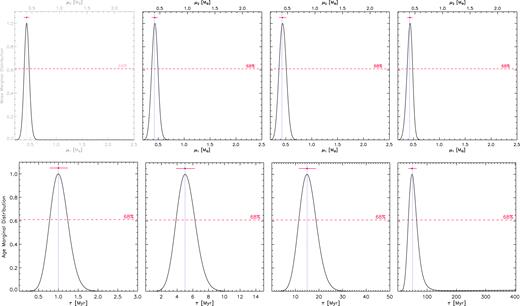
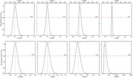
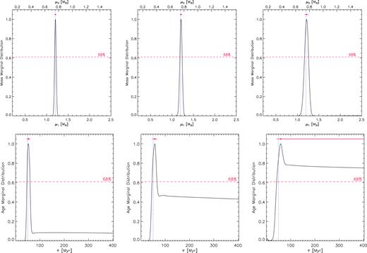
Mass (upper row) and age (lower row) marginal distributions for the simulated SB2 system X0.9, obtained with MR uncertainty |$\sigma_{{\it \mathrm{ MR}}}$| = 0.01, temperature error |$\sigma_{T_{\rm eff}}$| = 100 K, and gravity error σlogg= 0.10 dex. From left to right, panels on the first column refer to results at 1 Myr, on the second column at 5 Myr, on the third column at 15 Myr, and on the fourth column at 50 Myr. As to mass marginal distributions, lower abscissa refers to primary component and upper abscissa to secondary component. Red dots and dotted blue lines indicate the Bayesian results and the real values, respectively. Horizontal dashed lines represent the confidence level; horizontal red solid lines are the corresponding CIs.
Marginal distributions for the simulated SB2 system Y0.9. See caption of Fig. 1 for details.
Marginal distributions for the simulated SB2 system X0.6. See caption of Fig. 1 for details.
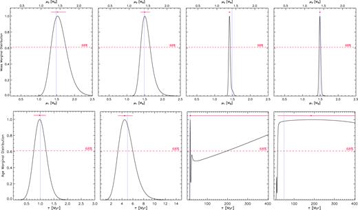
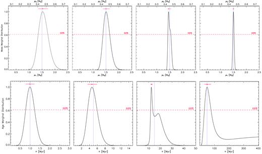
Marginal distributions for the simulated SB2 system Y0.6. See caption of Fig. 1 for details.
Marginal distributions for the simulated SB2 system X0.3. See caption of Fig. 1 for details.
Marginal distributions for the simulated SB2 system Y0.3. See caption of Fig. 1 for details.
Bayesian results and CI at 68 per cent confidence level for the simulated SB2 systems. Asterisk means that the limit of the CI is not determined in our age range.
| τs (Myr) | M1, Bayes (M⊙) | CI for M1, Bayes | M2,Bayes (M⊙) | CI for M2,Bayes | τs, Bayes (Myr) | CI for τs, Bayes |
|---|---|---|---|---|---|---|
| X0.9, M1 = 0.42 M⊙, M2 = 0.40 M⊙, MR = 0.95 | ||||||
| 1.00 | 0.43 | [0.38, 0.48] | 0.40 | [0.36, 0.45] | 1.00 | [ 0.78, 1.23] |
| 5.01 | 0.43 | [0.37, 0.49] | 0.41 | [0.35, 0.47] | 5.01 | [ 3.87, 6.26] |
| 14.96 | 0.44 | [0.37, 0.51] | 0.41 | [0.35, 0.48] | 14.96 | [11.44, 18.73] |
| 50.12 | 0.44 | [0.38, 0.49] | 0.41 | [0.36, 0.46] | 48.42 | [35.79, 64.04] |
| Y0.9, M1 = 1.49 M⊙, M2 = 1.40 M⊙, MR = 0.94 | ||||||
| 1.00 | 1.52 | [1.34, 1.76] | 1.43 | [1.26, 1.65] | 0.98 | [ 0.76, 1.21] |
| 5.01 | 1.50 | [1.38, 1.65] | 1.41 | [1.30, 1.55] | 4.47 | [ 3.25, 5.99] |
| 14.96 | 1.41 | [1.39, 1.44] | 1.33 | [1.31, 1.35] | 14.96 | [13.72, 400*] |
| 50.12 | 1.49 | [1.47, 1.51] | 1.40 | [1.38, 1.42] | 184 | [18.71, 400*] |
| X0.6, M1 = 1.20 M⊙, M2 = 0.75 M⊙, MR = 0.63 | ||||||
| 1.00 | 1.22 | [1.08, 1.38] | 0.76 | [0.68, 0.86] | 0.99 | [ 0.77, 1.22] |
| 5.01 | 1.20 | [1.11, 1.30] | 0.75 | [0.70, 0.81] | 4.79 | [ 3.61, 6.12] |
| 14.96 | 1.21 | [1.12, 1.31] | 0.76 | [0.70, 0.82] | 14.13 | [11.24, 17.56] |
| 50.12 | 1.21 | [1.18, 1.24] | 0.76 | [0.74, 0.77] | 56.89 | [45.38, 65.87] |
| Y0.6, M1 = 1.70 M⊙, M2 = 1.06 M⊙, MR = 0.62 | ||||||
| 1.00 | 1.74 | [1.53, 1.98] | 1.09 | [0.96, 1.24] | 0.98 | [ 0.77, 1.22] |
| 5.01 | 1.71 | [1.59, 1.86] | 1.07 | [0.99, 1.16] | 4.68 | [ 3.66, 5.86] |
| 14.96 | 1.70 | [1.67, 1.73] | 1.06 | [1.04, 1.08] | 14.79 | [13.23, 16.47] |
| 50.12 | 1.71 | [1.68, 1.74] | 1.07 | [1.05, 1.09] | 30.20 | [27.11, 362] |
| X0.3, M1 = 1.00 M⊙, M2 = 0.30 M⊙, MR = 0.30 | ||||||
| 1.00 | 1.02 | [0.89, 1.16] | 0.31 | [0.27, 0.35] | 0.99 | [ 0.77, 1.22] |
| 5.01 | 1.01 | [0.91, 1.11] | 0.30 | [0.27, 0.33] | 4.84 | [ 3.70, 6.16] |
| 14.96 | 1.02 | [0.94, 1.11] | 0.30 | [0.28, 0.33] | 13.65 | [ 9.87, 17.79] |
| 50.12 | 1.00 | [0.97, 1.04] | 0.30 | [0.29, 0.31] | 48.98 | [32.83, 69.62] |
| Y0.3, M1 = 1.50 M⊙, M2 = 0.45 M⊙, MR = 0.30 | ||||||
| 1.00 | 1.53 | [1.35, 1.72] | 0.46 | [0.41, 0.52] | 0.99 | [ 0.77, 1.22] |
| 5.01 | 1.50 | [1.39, 1.65] | 0.45 | [0.42, 0.49] | 4.62 | [ 3.52, 5.95] |
| 14.96 | 1.46 | [1.43, 1.55] | 0.44 | [0.43, 0.46] | 12.45 | [11.68, 13.57] |
| 50.12 | 1.50 | [1.48, 1.53] | 0.45 | [0.44, 0.46] | 50.12 | [31.75, 76.84] |
In principle, one could think that the age is accurately estimated for a system with masses sufficiently different to be in very different evolutionary stages, since the product of the likelihoods of the two components results in a well-defined peak. That is, the smaller the MR, the better the Bayesian age determination. However, this statement is not always true. As an example, age estimation for X0.9 and Y0.6 at 50 Myr is well derived only in the former case (Table 2). Indeed, the reliability of Bayesian results is related to the position of components on the plane of the observables. By referring to the Hertzsprung–Russell (HR) diagram for simplicity, along an isochrone (track), stellar mass (age) changes with Teff and L, and the mass (age) gradient can be defined as the sum of their partial derivatives. Since these gradients are not constant on the HR diagram, if we define a Teff– L error box due to observational uncertainties (as in GPT12) and imagine to move it on the Teff–L plane, we expect precise Bayesian estimations where the box encircles regions with a small gradient (i.e. where different points identified by close observable values refer to very similar masses or ages); on the contrary, in regions with a large gradient, we expect to obtain unreliable Bayesian results (since different points identified by close observable values refer to very different masses or ages). In conclusion, the smaller the mass (age) gradient along an isochrone (track), the better the precision on Bayesian mass (age) estimation. For PMS stars, the evolution along the Hayashi Track is slower than along the Henyey Track. This means that the age gradient in the Hayashi Track is larger than in the Henyey Track, so that in the latter phase the age will be better derived than in the former one. When a star is approaching the main sequence (MS), stellar parameters change slowly in time and the precision of age determination gets worse.
Anyway, in a real case, it is not possible to know a priori where components lie on the HR diagram. Luckily, the goodness of Bayesian results can be generally testified by the shape of marginal distributions. As to coevality, for example, the absence of a well-defined peak and a constant trend over a large time range (case Y0.9 at 50 Myr) outline the constancy of stellar parameters of both components now in the MS phase (see upper panels of Fig. 7) and that the Bayesian analysis cannot help. If only the primary has started the MS phase, the age marginal distribution presents a peak meaning that the secondary star dates the system. This is what happens for Y0.6 at 15 Myr and Y0.3 at 50 Myr: their primary components are already in the MS, while secondary stars lie, respectively, at the beginning of the Henyey Track (Fig. 7, left third panel from the top) and at the end of the Hayashi Track (Fig. 7, left lower panel). In both cases, the age marginal distribution shows a peak corresponding to the actual value (see Fig. 7, right third panel from the top and right lower panel). An interesting result is represented by Y0.6 at 50 Myr, where again the secondary star dates the system, but the peak (Fig. 7, right second panel from the top) indicates a coevality of 30 Myr. In the same figure (left second panel from the top), an isochrone of a slightly lower age has been plotted to show that 30 Myr is just the theoretical value from when observational parameters of the secondary star remain constant. Without a useful contribution from the primary in deriving the age, for this unlucky case the coevality is underestimated.
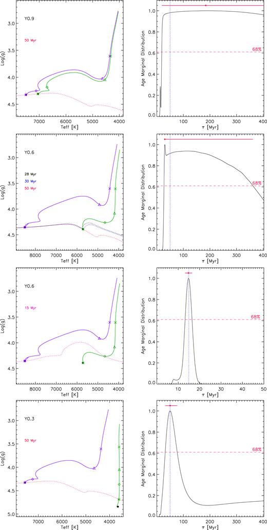
Left column: time trend of logg versus Teff for primary (violet solid line) and secondary (green solid line) components of the systems Y0.9 (upper panel), Y0.6 (second and third panels from the top), and Y0.3 (lower panel). Dotted lines are the isochrones at the indicated ages, symbols mark the pairs (Teff, logg) at age 1 Myr (×), 5 Myr (▵), 15 Myr (⋄), and 50 Myr (*). Black filled circles indicate the zero-age main-sequence values. Right column: age marginal distributions at 50 Myr for the simulated SB2 systems Y0.9 (upper panel), Y0.6 (second panel from the top), Y0.3 (lower panel), and at 15 Myr for Y0.6 (third panel from the top), obtained with MR uncertainty |$\sigma_{{\it \mathrm{ MR}}}$| = 0.01, temperature error |$\sigma_{T_{\rm eff}}$| = 100 K, gravity error σlogg = 0.10 dex. Red dots and dotted blue lines indicate, respectively, the Bayesian results and the real values. Horizontal dashed lines represent the confidence level; horizontal red solid lines are the corresponding CIs.
Nevertheless, despite a marginal distribution presents a well-defined peak, in some cases the Bayesian value could slightly differ from the real one. This happened for mass estimations of Y0.9 at 15 Myr, for which the worst mass recovery has been obtained (Table 2 and Fig. 2).
To point out the advantages in using the MR prior distribution (MR prior) with respect to no information about masses (flat mass prior), we applied the analysis on the previous systems for this last case too, with the above-mentioned errors (Section 3). By setting a flat ξ(μ1, μ2) function, we determined the mass of each component from equation (4), and their coevality as the mode of the product between primary and secondary age marginal distributions (equation 5), i.e. GC(τ) = G1(τ) × G2(τ) (GPT12).
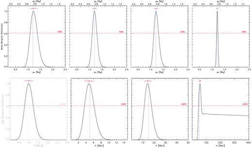
Fig. 8 shows the marginal distributions obtained with both flat mass prior (top panels) and MR prior (middle panels) for the system Y0.6 at 15 Myr. Comparison between the two cases highlights how the introduction of the MR information, in addition to providing better mass estimations, reduces the CI.
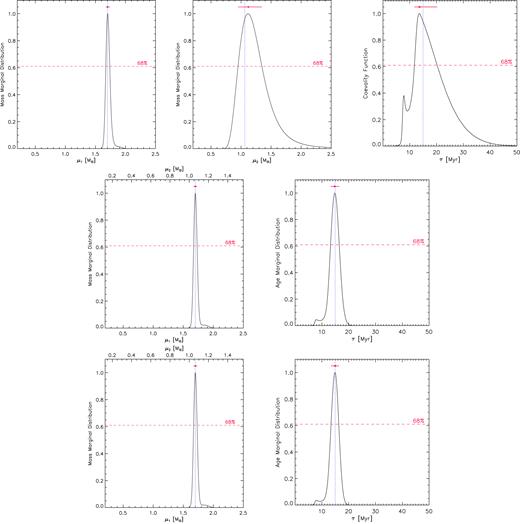
Marginal distributions for the simulated SB2 system Y0.6 at 15 Myr, obtained with temperature uncertainty |$\sigma_{T_{\rm eff}}$| = 100 K, gravity uncertainty σlogg = 0.10 dex. The flat case is shown in the top panels for primary mass (left-hand panel), secondary mass (central panel), and coevality (the function GC(τ) = G1(τ) × G2(τ), right-hand panel). The MR case results are plotted in the middle panels (|$\sigma_{{\it \mathrm{ MR}}}$| = 0.01) and in the bottom panels (|$\sigma_{{\it \mathrm{ MR}}}$| = 0.001): left-hand panels show the mass marginal distributions of both stars (lower abscissa for primary component and upper abscissa for secondary component) and right-hand panels show the age marginal distributions of the system. See caption of Fig. 7 for symbol meaning.
3.3 Input uncertainties
We explored a possible dependence of results on temperature, gravity, and MR uncertainties. For this purpose, we applied the analysis to all systems by combining |$\sigma_{T_{\rm eff}}$| = 50, 100, and 200 K, σlogg = 0.05, 0.10, and 0.20 dex, and |$\sigma_{{\it \mathrm{ MR}}}$| = 0.01 and 0.001.
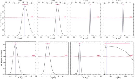
A comparison between marginal distributions obtained with different temperature and gravity errors for the system X0.6 at 50 Myr is shown in Fig. 9. As expected, the higher the input uncertainties, the larger the CI as well as the worse the Bayesian result.
Mass (top) and age (bottom) marginal distributions for the simulated SB2 system X0.6 at 50 Myr, obtained with MR uncertainty |$\sigma_{{\it \mathrm{ MR}}}$| = 0.01, temperature and gravity uncertainties |$\sigma_{T_{\rm eff}}$| = 50 K and σlogg = 0.05 dex (left-hand panels), |$\sigma_{T_{\rm eff}}$| = 100 K and σlogg = 0.10 dex (central panels), and |$\sigma_{T_{\rm eff}}$| = 200 K and σlogg = 0.20 dex (right-hand panels). See captions of Figs 7 and 8 for the layout.
Differences between marginal distributions obtained with the two |$\sigma_{{\it MR}}$| values are negligible, as shown in Fig. 8 (middle and bottom panels) for the system Y0.6 at 15 Myr. It means that the typical error in MRs is not dominant in deriving Bayesian results with respect to other uncertainties.
3.4 On the CI definition
With reference to a generic marginal distribution curve F(x) defined in the range [xmin, xmax] and normalized to the unit at the mode |$\hat{x}$|, |$F(\hat{x}$|) = 1, JL05 demonstrated how for a normal distribution, or at least under the validity of their equation (14), a given confidence level corresponds to a function value Flim (e.g. Flim = 0.61 gives the 68 per cent confidence level). The Flim value allows to define the CI of the retrieved Bayesian estimation as the interval [xi, xf] outside of which it always is F(x) < Flim. If the function exceeds Flim at xmin (xmax), JL05 set xi = xmin (xf = xmax), meaning that no lower (upper) limit at the chosen confidence level can be estimated. Anyway, a Bayesian marginal distribution could be very different from a Gaussian, and the authors computed numerical simulations to check the validity in assuming equation (14) for practical cases.
In order to adopt the same definition, we also made a numerical test as it follows: for the marginal distributions derived in our analysis, we computed the CIs corresponding to Flim from 0.1 to 0.9 at step of 0.1 using equation (14). We then applied the Bayesian procedure to each system 1000 times by adding random normal values to the observational quantities and looked for the number of mass and age estimations within the computed CIs. Results are plotted in Fig. 10: the general trend of simulations reproduces quite well the theoretical one from equation (14) (solid curve). As it was for JL05, only few cases are not in agreement, namely, Y0.9 at 15 and 50 Myr and Y0.3 at 15 Myr. In particular, for Y0.9 at 15 and 50 Myr, an upper limit of the age cannot be given at the chosen confidence level (see Table 2 and Fig. 2).
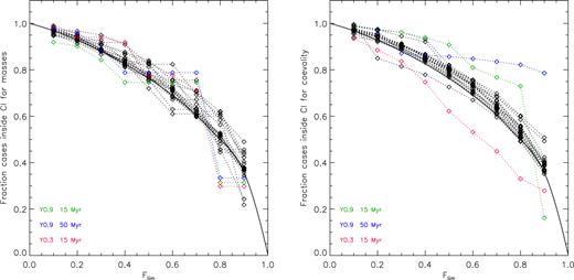
Results of the numerical simulations discussed in Section 3.4. The ordinate represents the fraction of masses (left-hand panel) and age (right-hand panel) within the CI corresponding to the Flim in abscissa. Each symbol (⋄) indicates the statistics from 1000 simulations. The solid curve shows the theoretical trend according to equation (14) of JL05.
4 APPLICATION TO REAL CASES: PAR 1802 AND RX J0529.4+0041 A
In this section, we discuss the results of our method for two real PMS binary systems, namely, Parenago 1802 (Par 1802) and RX J0529.4+0041 A. These are dESB2 in the Orion nebula Cluster (ONC) (Cargile, Stassun & Mathieu 2008; Gómez Maqueo Chew et al. 2012, hereafter G12) and Ori OB1a association (Covino et al. 2000, hereafter C00), respectively.
For both systems, we assumed metallicity Zobs = 0.0123 ± 0.0030 from the measured [Fe/H] = − 0.02 ± 0.10 dex (Nieva & Simón-Díaz 2011).
To apply our method, we treated each of them as an SB2 by assuming the MR obtained from the amplitudes K1 and K2 of the radial velocity variation of the two components, MR = K1/K2. Then we compared the Bayesian masses with the known dynamical ones and the resulting age with the value from literature.
Concerning Par 1802, we adopted the most recent physical parameters provided by G12, i.e. MR = 0.984 ± 0.085, |$T_{\rm eff_{1}}$| = 3675 ± 150 K, log|${g}_{_1}$| = 3.55 ± 0.04 dex, and |$T_{\rm eff_{2}}$| = 3365 ± 150 K, log|${g}_{_2}$| = 3.61 ± 0.04 dex. We obtained Bayesian masses M1, Bayes = 0.409 M⊙ with CI = [0.329, 0.491] M⊙, M2, Bayes = 0.403 M⊙ with CI = [0.324, 0.483] M⊙, and coevality τs, Bayes = 1.04 Myr with CI = [0.94, 1.15] Myr. These values well agree with the dynamical masses, namely, 0.391 ± 0.032 and 0.385 ± 0.032 M⊙, derived by G12 for primary and secondary components, respectively, and with the estimated age < 1 − 2 Myr of the ONC (Hillenbrand 1997).
For RX J0529.4+0041 A, we adopted physical parameters provided by Covino et al. (2004, hereafter C04), i.e. MR = 0.730 ± 0.003, |$T_{\rm eff_{1}}$| = 5200 ± 150 K, log|${g}_{_1}$| = 4.22 ± 0.02 dex, and |$T_{\rm eff_{2}}$| = 4220 ± 150 K, log|${g}_{_2}$| = 4.14 ± 0.02 dex. The same authors determined dynamical masses 1.27 ± 0.01 M⊙ for primary component and 0.93 ± 0.01 M⊙ for secondary component. Both C00 and C04 attributed to this system an age of nearly 10 Myr from the isochrones of different authors, compatible with the 7–10 Myr found for the hosting Ori OB1a association by Briceño et al. (2005). The agreement (within the CI) between their estimations and our Bayesian results, i.e. M1, Bayes = 1.22 M⊙ with CI = [1.16, 1.29] M⊙, M2, Bayes = 0.89 M⊙ with CI = [0.85, 0.94] M⊙, and τs, Bayes = 7.08 Myr with CI = [6.52, 7.67] Myr, confirms the validity of the method.
Marginal distributions for Par 1802 and RX J0529.4+0041 A are plotted in Fig. 11.

Since the results are also model-dependent, we mention here the paper by Stassun, Feiden & Torres (2014) who compared masses and age of PMS eclipsing binaries obtained with solar-calibrated models from different evolutionary codes (including franec). Despite some differences in the input physics, the authors found a general reliability in recovering the dynamical masses better than ∼10 per cent for all the examined models, and an average agreement with the franec age results within ∼20 per cent with the exception of the ∼30 per cent for the Baraffe et al. (1998) models.
5 CONCLUSIONS
We presented a method based on the Bayesian analysis of SB2s to estimate the system age and masses. Our procedure has been developed under the hypothesis of coevality and same initial chemical composition of the two components.
The method assumes the SB2 as a single object and exploits the MR as the a priori information about the masses of both its components. For these systems, in fact, it is not possible to obtain dynamical mass estimations. Moreover, the only physical independent parameters spectroscopically determinable for each star are effective temperature and surface gravity.
We numerically tested the procedure on a sample of simulated low-mass (M < 2 M⊙) PMS SB2s on the basis of stellar models computed with the evolutionary code franec. The advantage of introducing the MR prior probability, which leads to more precise results with respect to no information about masses, has been shown. By setting typical values of MR uncertainty, we found no relevant differences in our analysis, that is, the present MR errors are not dominant in deriving Bayesian results. By applying the procedure with different combinations of temperature and gravity uncertainties, we have shown that the higher the input errors, the larger the CI, as well as the worse the age and mass estimations.
The reliability of results can be generally testified by the shape of marginal distributions. In particular, the capability of the method in recovering the system age gets worse when both components are approaching the MS. The absence of a well-defined peak in the age marginal distribution of a star, in fact, does not allow to obtain an age estimation and tell us that the star has started the MS phase.
We finally applied the procedure to the PMS eclipsing binaries Parenago 1802 and RX J0529.4+0041 A with known dynamical masses, treated as SB2 systems. This allowed to test the reliability of Bayesian results based only on spectroscopic data.
The method we presented provides a mass value for the single components of the SB2 in exam as well as a system age estimation, enlarging the sample of stars with known fundamental parameters. It could then allow to date a large number of astrophysical environments by the hosted binary systems.
REFERENCES
in
