On the hydrostatic stratification of the solar tachocline

Abstract

1 INTRODUCTION

There is some ambiguity in helioseismological inferences about the spherically averaged stratification of the Sun in the vicinity of the base of the convection zone. Consequently, there is an associated uncertainty in the location of the base of the convection zone itself. Problems in interpreting helioseismological inversions of global frequency data arise because we are unsure of the dynamical consequences of convective overshoot, and of the influence of the magnetic field and of chemical-element segregation by gravitational settling moderated by the large-scale meridional flow in the tachocline. Issues such as these were recognized by Christensen-Dalsgaard, Gough & Thompson (1991) in their original attempt to locate the base of the convection zone, causing them to suggest that the real uncertainty in their estimate is substantially greater than the formal precision of their data analysis by a factor 3 or even more.

Christensen-Dalsgaard et al. adopted two different procedures for determining the radius r_c of the base of the convection zone: an absolute method, which used an asymptotic formulation of the entire sound-speed stratification of the star and which did not rely on a solar model, and a differential method, which used an asymptotic description of only the relatively small difference between the Sun and a standard theoretical model. The latter is naturally more precise, but it depends in a not wholly obvious manner on the approximations adopted in constructing the reference solar model. The conclusion from the differential method was r_c = 0.713 ± 0.003R, where R is the (photospheric) radius of the Sun. Subsequently, Basu & Antia (1997) carried out a broadly similar asymptotic differential analysis with more precise frequency data, obtaining r_c = 0.713 ± 0.001R. It is essential to understand that the quoted errors indicate only the precision of the analysis, and may have little bearing on the accuracy of the calibration. Unfortunately, the distinction between the two has not always been appreciated.

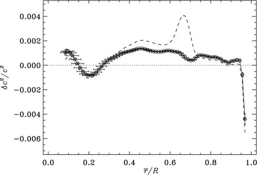
Gyroscopic pumping associated with rotational shear in an essentially radiatively stratified layer beneath the convection zone (Spiegel 1972; Spiegel & Zahn 1992) exchanges material in that layer with the convection zone, thereby opposing the tendency of gravitational settling to establish a gradient of helium and heavier elements. This process, which must inevitably be taking place, although possibly in tandem with other mixing processes, tends to reduce abundance gradients on a time-scale almost certainly less than the local characteristic settling time (Gough & McIntyre 1998). The outcome is to make the spatial variation of the helium abundance Y rather smoother than in standard theoretical models, resulting in a positive anomaly (acoustical glitch) in the difference between the sound speeds in the Sun and the models. Such a glitch is evident in differential inversions of helioseismic data against standard solar models, as is illustrated in Fig. 1, and has been recognized also by Antia & Chitre (1998) as being a signature of material mixing.

Figure 1.

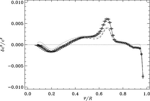
The symbols depict optimally localized averages of the relative difference between the squared sound speed in the Sun and that in the new Model S, in the sense (Sun) – (model), which was constructed with the opacities of Iglesias & Rogers (1996) and calibrated to Z_s/X_s = 0.0245, corresponding to the heavy-element abundances of Grevesse & Noels (1993); they are plotted against the centres |$\overline{r}$| of the averaging kernels and joined by straight-line segments. The horizontal bars indicate the widths of the averaging kernels, and the vertical bars denote standard errors arising from the uncertain errors, assumed to be independent, in the observational data (obtained from Basu et al. 1997). The dashed curve is drawn through similar averages of the relative difference between c² in the Sun and that in the original Model S (Christensen-Dalsgaard et al. 1996), which was constructed with the opacities of Rogers & Iglesias (1992a,1992b) and calibrated also to Z_s/X_s = 0.0245. The dotted curve similarly shows results from an analysis of a model (Model S΄; see Section 5) computed with the opacities of Iglesias & Rogers (1996), the relative heavy-element abundances of Asplund et al. (2009), calibrated to Z_s/X_s = 0.0181 and including the opacity modification of Christensen-Dalsgaard & Houdek (2010).

Open in new tabDownload slide

If essentially laminar tachocline circulation were the only homogenizing agent, it would be possible in principle to determine the thickness of the tachocline from the properties of the acoustical glitch. A calibration of the dimensions of the glitch is likely to be more precise than analyses of rotational splitting, for example, because the mean multiplet oscillation frequencies that are employed have been determined from observation more precisely than has rotational splitting. However, the outcome is not necessarily more accurate, because it is conditional on the assumptions of the stellar modelling, both on the physical approximations adopted in constructing the standard reference solar model and on the structure adopted for the tachocline, now and throughout the earlier evolution of the Sun.

A calibration of the glitch was attempted by Elliott & Gough (1999) and Elliott, Gough & Sekii (1998), who adopted what one might regard as the simplest of assumptions: namely that the stratification of the Sun is spherically symmetrical, that material mixing is complete down to the base of the tachocline at a rate that does not disturb radiative equilibrium, essentially in conformity with the tachocline model of Gough and McIntyre (1998), sometimes referred to as a slow tachocline, and that the thickness Δ of the tachocline has not changed throughout the main-sequence lifetime of the Sun, together, of course, with the other standard assumptions of solar modelling (Christensen-Dalsgaard et al. 1996). They found that Δ = 0.020R, the formal uncertainty in that value, resulting from only the quoted uncertainties in the seismic frequency data, being about 5|$\,{per\,cent}$|⁠.

Elliott and Gough were encouraged by their finding that not only the height and width of the acoustic glitch but also its functional form could be reproduced within the formal errors by adjusting but a single parameter Δ. That provided some, yet unjustified, modicum of faith in their result. However, the glitch in the calibrated model was displaced upwards by 0.015R from that in the reference model, the consequences of which we discuss in the next section. With what now appears to be the false confidence in their partial success, they presumed that the calibration of Δ was reliable and that the fully mixed region was deeper than earlier analyses had indicated.

It was never intended to be believed that the simplistic tachocline modelling of Elliot and his colleagues, based on the minimalist analysis of Gough and McIntyre (1998), should be strictly trusted. Other processes are also operative, not least of which is convective overshoot, which smears the mathematically precise location of both the base of the convection zone and the tachopause, beneath which in the simplistic model there was supposed to be no fluid motion. It was accepted that temporally varying overshoot of descending convective plumes must occur, but it was assumed that its long-term effect was small compared with that of the large-scale tachocline flow. In contrast, others have argued either that overshoot (e.g. Berthomieu et al. 1992) or rotationally driven shear turbulence (e.g. Richard et al. 1996; Brun, Turck-Chièze & Zahn 1999) provides the principal source of material redistribution, possibly in the manner of an effective diffusion, and that it dominates the tachocline flow in smoothing the abundance profiles. No such assumption appears to have succeeded in removing the acoustic anomaly entirely (e.g. Brun et al. 2002; Brun & Zahn 2006).

Although the difference between the sound speed in the Sun and that in standard solar models is, by many astrophysical standards, extremely small, it is very much larger than the standard errors in the determinations of the sound speed (in places by as much as 20 formal standard errors in the helioseismological inversions). Therefore, the discrepancies are very significant and demand explanation. Those discrepancies can quite easily be separated into two components: one that varies on a length-scale comparable with the size of the Sun, and is no doubt a consequence of gross, albeit small, errors in properties that influence the global structure, such as the primordial chemical composition, the treatment adopted for the opacity, which controls the radiative transfer of energy, or the dominant nuclear cross-sections, and one that is local and is produced by errors in the treatment of processes that influence the sound speed directly. The tachocline anomaly is the more prominent member of the latter component and is the subject of the investigation reported here.

It has long been appreciated that a spatially confined sound-speed anomaly is most likely to be a result of an error in the pressure–density relation adopted in the reference solar model, whose influence on the sound speed c = (γ₁p/ρ)^1/2 is direct. Here, p is the pressure, ρ is the density, and |$\gamma _1=({\partial} \,{\rm ln}\, p/{\partial} \,{\rm ln}\rho )_{\rm ad}$| is the first adiabatic exponent. Such an error could arise from an error in the concentrations of the abundant elements, which influences the mean molecular mass μ. In contrast, an error in the opacity or a controlling nuclear reaction rate influences the stratification only via coefficients that multiply derivatives in the governing differential equations, and therefore has more spatially extensive consequences (e.g. Elliott & Gough 1999). Although there is well appreciated uncertainty in the physics of the equation of state relating p to ρ, which might well be of a magnitude comparable with the sound-speed anomaly considered here (e.g. Däppen, Lebreton & Rogers 1990; Christensen-Dalsgaard & Däppen 1992; Baturin et al. 2000), it is quite unlikely that it would be restricted to a narrow region in the p–ρ relation, particularly the region that happens (by chance, from a thermodynamical point of view) to coincide with the base of the solar convection zone. Therefore, the most likely culprit is the spatial variation of the relative abundances of the most abundant chemical elements – helium and hydrogen – for only they have a sufficiently strong influence on the equation of state. Our task is therefore to examine that variation, a variation which is determined by the balance of overshoot, shear turbulence, wave transport and baroclinic tachocline flow against diffusion and settling. Here, we do not address the dynamical matters directly, but instead we attempt to determine the seismological consequences of putative mixing processes, and compare them with observation, in the hope that our conclusions will provide useful constraints on dynamical studies to come.

The large-scale global structure of calibrated solar models is influenced directly by the opacity, which controls the radiative interior, and indirectly by the location of the base of the convection zone, which is formally determined by conditions locally. The latter was realized early in the days of helioseismology from comparisons between theoretical solar models (e.g. Christensen-Dalsgaard 1988); the former came prominently into attention with the announcement by Asplund et al. (2004) that the abundance Z of heavy elements, and therefore the opacity produced from them, is substantially lower than had previously been believed (at least in the photosphere and the well mixed convection zone), thereby augmenting the discrepancy between the seismologically determined stratification of the Sun and that of standard solar models, such as Model S of Christensen-Dalsgaard et al. (1996). An extended review of these issues is provided by Basu & Antia (2008). Attempts to compensate for Asplund’s revised composition have not been successful within the realm of currently accepted physics (Guzik & Mussack 2010). However, given that the composition affects predominantly the opacity, modifications to opacity with no a priori physical basis can be adjusted to cancel the effects of the composition change to bring models back to Model S (Christensen-Dalsgaard et al. 2009; Christensen-Dalsgaard & Houdek 2010), leaving the tachocline anomaly intact.

To relate our current investigation to earlier studies, we first investigate simple attempts to bring Model S into better agreement with the seismically inferred sound-speed stratification. We then consider the effect on models computed with the Asplund et al. (2009) composition of adjusting the opacity in the radiative interior and subsequently the degree of material mixing in the tachocline, both without regard to how such adjustments might be accomplished physically, in an attempt simply to reproduce that stratification.

2 THE TACHOCLINE ANOMALY

In Fig. 1 is depicted the difference in the squares of the sound speeds in the Sun and in a new standard solar Model S, the latter having been computed and calibrated in the same manner as the original Model S of Christensen-Dalsgaard et al. (1996), including a present ratio Z_s/X_s = 0.0245 between the surface abundances by mass of heavy elements and hydrogen (Grevesse & Noels 1993), but using the more modern OPAL opacities of Iglesias & Rogers (1996).¹ The initial heavy-element abundance is Z₀ = 0.0196, the same as in the original Model S. For comparison, we include a plot of differences from the original Model S. Throughout this paper, the term Model S refers to the new model, unless explicitly stated otherwise. For completeness, we note that the model is calibrated to a photospheric radius of 6.9599 × 10¹⁰ cm and surface luminosity of 3.846 × 10³³ erg s⁻¹ at an age of 4.6 Gyr. The equation of state used the OPAL tables of Rogers, Swenson & Iglesias (1996) and nuclear parameters mostly from Bahcall, Pinsonneault & Wasserburg (1995). Diffusion and settling of helium and heavy elements, at the rate of fully ionized oxygen, were included using the approximation of Michaud & Proffitt (1993). Plotted in Fig. 1 are optimally localized averages (e.g. Gough 1985; Gough & Thompson 1991; Rabello-Soares, Basu & Christensen-Dalsgaard 1999) of those differences, which are averages weighted with Gaussian-like weight functions (commonly called averaging kernels) centred about |$\overline{r}$| with widths indicated by the horizontal bars; specifically, these extend from the first to the third quartiles of the averaging kernels, with a separation of around 0.57 times the full width at half maximum of the kernels. The vertical bars denote standard errors resulting from the quoted errors in the observed frequencies, computed under the assumption that the errors in the observations are independent. The inverse analysis was carried out in terms of the pair (c², ρ). To facilitate comparison with earlier analyses (e.g. Christensen-Dalsgaard & Di Mauro 2007), here and in the following we use the same observational data as did Basu et al. (1997).

We discuss first the prominent hump centred at |$\overline{r}\simeq 0.67 R$| immediately beneath the convection zone where the tachocline is located. Elliott and Gough (1999) called it the tachocline anomaly, because they believed it to be a product of tachocline mixing, and we adopt that nomenclature here.

The discrepancy was postulated to have been caused by the tachocline circulation, which returns settling helium to the convection zone, thereby locally augmenting the hydrogen abundance, and with it the sound speed. The fact that Elliott and Gough had found that the anomaly, although located too high in the envelope, could otherwise be reproduced by adjusting only the single parameter Δ led them naively to suppose that the structure had been predicted robustly, and that the anomaly could simply be shifted downwards by global adjustments to the model that deepened the convection zone. Consequently, they made no attempt to construct a fully self-consistent calibrated evolutionary model. However, as we demonstrate in the next section, a self-consistent model with a Gough-McIntyre tachocline that is not contradicted by seismology cannot be constructed in so simple a fashion. This should have been anticipated, because it has long been known that changing the depth of the convection zone in a model would introduce an additional sharp feature in the sound-speed difference (Christensen-Dalsgaard 1988), manifest as a discrepancy in the sound-speed gradient that is concentrated principally in and immediately beneath the region in which one model is radiative and the other is convective; however, the sound-speed perturbation itself extends deep into the radiative interior. We discuss these aspects in some detail in the following sections. To bring the model in line with seismic observation, alternative features, to which we return in Section 5, need to be included in the model.

3 THE EFFECT OF SLOW TACHOCLINE MIXING ON HYDROSTATIC STRATIFICATION

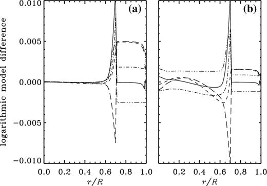
Fig. 2(b) depicts deviations from Model S (which we denote by δ below) at fixed r/R of ln c², ln p, ln ρ, ln T, where T is temperature, and the hydrogen abundance X in a properly calibrated solar model – reproducing the observed values of the luminosity, L_⊙, the radius, R_⊙, and a heavy-element–to–hydrogen abundance ratio, Z_s/X_s = 0.0245, in the photosphere – having a slow tachocline modelled by mixing the chemical composition in a layer 0.02R thick beneath and contiguous with the convection zone, yet retaining radiative equilibrium. We note that, as detailed in the Appendix, the sound speed in the bulk of the convection zone is largely fixed by the surface mass and radius of the model, such that here δc² ≈ 0. Thus, the mixing of otherwise gravitationally settled material, causing a reduction in the hydrogen abundance in the convection zone with a consequent augmentation of the mean molecular mass μ, is compensated by a corresponding augmentation of T. For comparison, we include a similarly constructed model with the same initial heavy-element abundance, Z₀ = 0.0196, as Model S; in that model the value of Z_s/X_s is 0.0249, which differs from 0.0245 by much less than the observational uncertainty (Grevesse & Noels 1993).

Figure 2.

Differences at fixed r/R in ln c² (continuous curve), ln p (short dashed), ln ρ (long dashed), ln T (dot–dashed), and X (triple-dot–dashed) between the model with a slow tachocline, described in Section 3, and Model S. The model in panel (a) was computed with the same Z₀ as Model S, namely 0.0196; the model in panel (b) was calibrated to the same present value of Z_s/X_s, namely 0.0245.

Open in new tabDownload slide

Had the initial heavy-element abundance Z₀ been held constant in the calibration, these modifications to the outer layers of the star would have had little influence on conditions deep in the radiative envelope and the energy-generating core, and all the perturbations would have declined towards zero (Fig. 2a). It is evident from the equation of hydrostatic support in the form d ln p/d r = −γ₁ Gm/c²r², where m is the mass within a radius r and G is the gravitational constant, that the raised sound speed in the acoustic glitch would have reduced the magnitude of the pressure gradient, thereby causing the pressure, and concomitantly the density, in the convection zone to be increased. In the tachocline itself, p/ρ would have been increased, requiring an even greater inwards reduction in ln ρ than in ln p. These changes induce lesser, compensating, deviations with reversed sign in a transition zone beneath, as depicted in Fig. 2.

The reduced surface abundance X_s caused by the tachocline circulation leads to a reduced heavy-element abundance Z_s in a calibration at fixed Z_s/X_s, a reduction which is transmitted throughout the entire star. The resulting diminution of the opacity in the radiative interior leads to a global reduction in temperature, and a reduction of p and ρ in the outer radiative envelope and convection zone, enough to reverse the sign of δln p and δln ρ in the convection zone. Consistent with the maintenance of hydrostatic support under homologous change, which approximately characterizes the modifications undergone by the recalibration, the reduction in T is balanced principally by a corresponding reduction in μ, therefore an augmentation in X, which maintains the nuclear reaction rates; the jump in X across the tachocline is hardly changed, so there is some mitigation of the reduction in X_s by the recalibration.

When δc² is convolved with the averaging kernels of the inversion (Fig. 3), the anomaly in this model appears to be centred higher in the envelope than the anomaly observed (see Fig. 1), by a little over 0.015R, at r = 0.685R, more-or-less as Elliott and Gough had found. This is because the anomaly is asymmetric with respect to r, and the kernel averages appear to broaden the steeper (upper) side of the anomaly more than they do the lower. A direct consequence of that property is a small, yet sharp, dip in the sound-speed difference immediately beneath the convection zone of the Sun. By what means can the location of the model anomaly be lowered?

Figure 3.

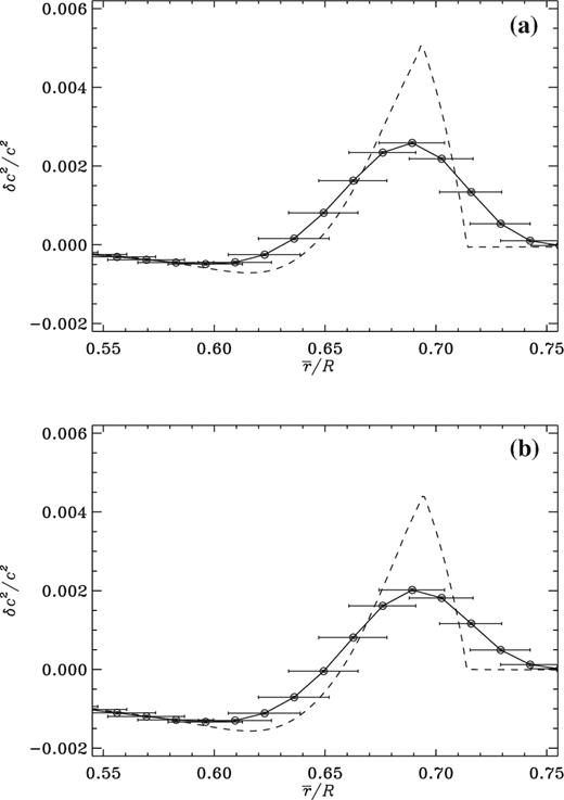
The symbols joined by continuous line segments represent the squared sound-speed difference plotted in Fig. 2, convolved with the optimal averaging kernels, and plotted against the centres of those kernels; the original squared sound-speed differences are reproduced here as dashed curves. The model in panel (a) was computed with the same Z₀ as Model S, the model in panel (b) was calibrated to the same present value of Z_s/X_s.

Open in new tabDownload slide

4 SIMPLE ADJUSTMENTS TO THE MODEL TACHOCLINE

One cannot simply imagine the adiabatically stratified region of the convection zone to be deepened without addressing how that could come about. Here, we restrict ourselves to the class of proposals most commonly encountered in discussions of the internal structure of the Sun: maybe there is non-locally driven, almost adiabatic, motion penetrating more deeply than the level of neutral stability, in the form of ‘fast’ large-scale tachocline flow or relatively local overshooting plumes that subsequently mix with their immediate surroundings; alternatively, for some reason, the opacity in the outer layers of the radiative zone is greater than is normally supposed, causing the local condition for convective instability to occur at a greater depth. We consider the two possibilities separately.

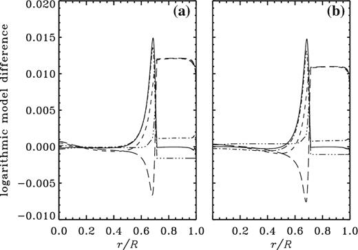
In Fig. 4 are plotted perturbations resulting from nearly adiabatic overshooting (or a fast tachocline), modelled by artificially extending the adiabatically stratified region of the convection zone by 0.015R and mixing the chemical composition with the convection zone. Because the magnitude of the temperature gradient in the extended layer is greater than its radiative counterpart, the temperature itself is greater. Therefore, the sound-speed anomaly is greater than that in a model with a slow tachocline of the same depth. The greater sound speed in the acoustic glitch requires a pressure-gradient perturbation of greater magnitude, and a consequent greater increase of pressure and density in the convection zone, rendering the deviations positive in the convection zone even when Z_s/X_s is held fixed in the recalibration. The strong concentration of the acoustic anomaly near the base of the convection zone renders this simple well mixed model incompatible with seismic inference.

Figure 4.

Differences in ln c² (continuous curve), ln p (short dashed), ln ρ (long dashed), ln T (dot–dashed), and X (triple-dot–dashed) between the model with a fast tachocline, or nearly adiabatic overshoot, and Model S. The model in panel (a) was computed with the same Z₀ as Model S, the model in panel (b) was calibrated to the same present value of Z_s/X_s.

Open in new tabDownload slide

Figure 5.

Differences in ln c² (continuous curve), ln p (short dashed), ln ρ (long dashed), ln T (dot–dashed), and X (triple-dot–dashed) between the model in which the opacity has been artificially augmented by the factor f (see equation 1) and Model S. The model in panel (a) was computed with the same Z₀ as Model S, the model in panel (b) was calibrated to the same present value of Z_s/X_s.

Open in new tabDownload slide

5 A SEARCH FOR A SEISMICALLY ACCEPTABLE MODEL

The devices discussed in the previous section to deepen the convection zone introduce changes in the sound speed that are concentrated near the base of the convection zone. They have broadly similar characteristics very close to the convection zone, in that they both produce a positive acoustic anomaly. The anomalies differ in their thickness–amplitude ratios, and their extensions deeper into the radiative interior are different. We are therefore moved to enquire whether an artificial modification to the opacity coupled with or replaced by a more gentle tachocline flow can be found to reproduce the observed sound-speed anomaly illustrated in Fig. 1.

Before proceeding with a discussion of the results of such an exercise, we recognize that analyses by Asplund et al. (2004), Asplund, Grevesse & Sauval (2005), and Asplund et al. (2009), and subsequently by Caffau et al. (2008, 2009, 2011), have resulted in a downward revision of Z_s. According to the latest results by Asplund et al. (2009), the reduction is approximately 25 per cent, yielding Z_s/X_s = 0.0181 ± 0.0008.² The effect on the equation of state is small, and has little influence on the stratification of a calibrated solar model. It is just the opacity κ that is affected. Christensen-Dalsgaard & Houdek (2010) computed a solar model with the same physics as Model S but with the revised value of Z_s obtained by Asplund et al. (2009), and they have demonstrated explicitly that an intrinsic modification Δlog κ to κ, assumed to depend just on T, can be found that converts its seismic structure to that of Model S. The opacity modification is otherwise arbitrary, but it is interesting to note that its value at least near the base of the convection zone is comparable with the revision in the iron opacity inferred recently from the Z-pinch experiment (Bailey et al. 2015; Nahar & Pradhan 2016).³ The result of a seismic analysis based on this model, Model S΄ in the following, is illustrated in Fig. 1 by the dotted line; it is evident that it closely resembles the original Model S. It appears, therefore, that it behoves us only to model the tachocline anomaly in its correct location. The analysis is based on using Δlog κ(T) as obtained by Christensen-Dalsgaard & Houdek (2010) together with the Asplund et al. (2009) composition, using Model S΄ as a starting point. We expect that a moderate further slight adjustment to κ would then suffice to remove any additional structural discrepancy at depth that may ensue. We now illustrate the extent to which we have been successful.

Here, we simply adopt the diffusion process and adjust D₀, |$v$|₀, and α in an attempt to obtain a satisfactory stratification beneath the convection zone. We illustrate the outcome in Fig. 6. There is no unique way of defining what one might consider to be a ‘best’ fit to the seismically determined structure. Here, we select a model with D₀ = 150 cm² s⁻¹, |$v$|₀ = 0.15 g⁻¹ cm³, and α = 4.25 throughout the main-sequence evolution, calibrated to have Z_s/X_s = 0.0181 at the present age of the Sun. This has successfully suppressed the tachocline anomaly, but at the expense of a somewhat larger deviation in the deeper seismically accessible regions of the radiative interior. As argued above, this smooth variation could in principle be suppressed by an appropriate modification to the opacity. Here, we have all but removed it in a new model obtained by simply augmenting Z_s/X_s in the model of the present Sun to 0.0189, at the limit of the assumed standard error in the composition determination by Asplund et al. (2009). The outcome is illustrated in Figs 7–9. The tachocline anomaly has almost disappeared.

Figure 6.

Relative sound-speed difference between the Sun and a model computed with the same physics as Model S΄, using the Asplund et al. (2009) composition and the opacity correction of Christensen-Dalsgaard & Houdek (2010), except that there has been added material diffusion beneath the convection zone with a diffusion coefficient D according to equation (2), with D₀ = 150 cm² s⁻¹, |$v$|₀ = 0.15 g⁻¹ cm³, and α = 4.25. The surface composition is characterized by Z_s/X_s = 0.0181. There remains a large-scale discrepancy in the radiative interior that can be largely removed by a suitable modification to the opacity. The dashed curve reproduces the deviation from Model S΄ illustrated in Fig. 1 by the dotted curve.

Open in new tabDownload slide

Figure 7.

As Fig. 6, except that the surface composition is characterized by Z_s/X_s = 0.0189. The small remaining large-scale discrepancy in the radiative interior can be largely removed by a suitable modification to the opacity.

Open in new tabDownload slide

Figure 8.

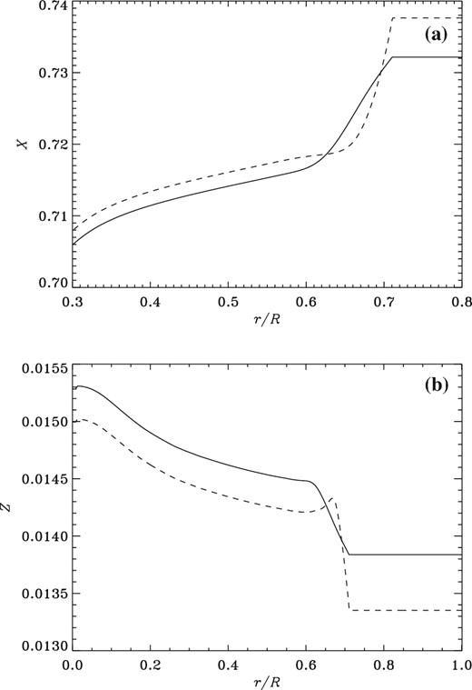
Abundance profiles of hydrogen, X, and heavy elements, Z, in the model illustrated in Fig. 7 with diffusive mixing, maintaining the radiative thermal stratification, immediately beneath the convection zone (continuous curves) and in Model S΄ (dashed curves).

Open in new tabDownload slide

Figure 9.

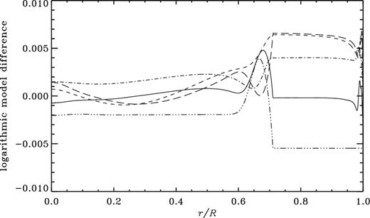
Differences in ln c² (continuous curve), ln p (short dashed), ln ρ (long dashed), ln T (dot–dashed), and X (triple-dot–dashed) between the model illustrated in Fig. 7 and Model S΄.

Open in new tabDownload slide

In Fig. 8 we compare the smoothed abundances X and Z of hydrogen and heavy elements in the new model with the corresponding abundances in Model S΄. Also, Fig. 9 shows relative differences between the two models. The overall effect of diffusive mixing is similar to that of the slow and fast tachocline discussed in Sections 3 and 4. The immediate consequence of mixing some of the settling material back into the convection zone, required for reducing the tachocline anomaly, is to reduce X in the convection zone, with a further reduction resulting from calibrating the model to a higher Z_s/X_s; this is coupled with a concomitant increase in temperature. The inclusion of diffusive mixing just beneath the convection zone has decreased the settling of both hydrogen and heavy elements. The more gradual decrease of the hydrogen abundance below the convection zone dominates the sound-speed difference, resulting in a peak which, when smoothed by the averaging kernels, closely matches the original tachocline anomaly found in the inversion using Model S΄. The change in calibration also leads to a general increase in Z and hence opacity, which is counteracted by an increase in temperature, maintaining the required radiative energy transport. The increase in temperature also largely balances the increase in mean molecular mass and hence, unlike the situation in Fig. 6, leads to a modest change in sound speed in the bulk of the radiative interior, where also Model S΄ provides a reasonable match to the helioseismologically inferred stratification.

6 DISCUSSION AND CONCLUSIONS

We have shown that material diffusion immediately beneath the convection zone, with a suitably chosen diffusion coefficient, can all but remove the acoustic glitch in solar Model S that arises principally from excessive gravitational settling of helium in the model. The partial chemical homogenization apparent in the spherically averaged structure to which the seismological analysis is sensitive could be the result of the tachocline circulation and possible convective overshooting, the latter having been caused in part by a true small-scale mixing and in part by a laminar undulation of the interface between the fully mixed convection zone and the relatively quiescent radiative interior, the details of which we have not studied.

We do not claim that we have necessarily determined the cause of the difference between Model S and the Sun in the tachocline region. There are certainly other possibilities, such as an error in the procedure adopted to model gravitational settling in Model S, an asphericity in the location of the base of the convection zone, or Stokes drift and Taylor dispersion by gravity waves generated at the base of the convection zone (e.g. Knobloch & Merryfield 1992), none of which have been investigated in detail.

A noteworthy feature in the difference between the solar and model structures, which persists in the model illustrated in Fig. 7, is the systematic variation below r ≈ 0.3 R. This is a region where, as illustrated by the horizontal bars, the resolution of the inversion is comparatively poor; in addition, there is substantial correlation between the inferences at different values of |$\overline{r}$| (e.g. Rabello-Soares et al. 1999), rendering the apparently smooth variation somewhat misleading. Even so, it is a common feature of helioseismological inferences, and hence likely to be of some physical significance. It is possible that it could be eliminated by a suitable modification to the opacity. However, it is interesting that it occurs in a region where the hydrogen abundance has been substantially modified by nuclear fusion, raising the possibility that additional weak mixing has occurred (e.g. Gough & Kosovichev 1990).

Our goal in this paper has been to elucidate the possible features that may affect the tachocline anomaly without introducing other discrepancies between the inferred solar sound-speed stratification and the model. This is the background for using data and model physics that have been extensively studied in the past but are no longer up to date. A more definitive analysis should be based on the most recent observational frequencies, such as those provided by Reiter et al. (2015). We note, however, that the inverse analysis presented in that paper shows differences between the Sun and Model S very similar to our starting point in Fig. 1. Furthermore, the model physics, and the assumed surface composition, should be updated (e.g. Vinyoles et al. 2017). Additional constraints on the properties of the tachocline region can be obtained by carrying out inverse analyses in terms of different pairs of variables characterizing the model structure; an interesting analysis in terms of the Ledoux discriminant has been presented by Buldgen et al. (2017). It seems likely that the results of these analyses will still, as in our preliminary work, point to a combination of modifications to the opacity and suitable transport processes changing the local composition (see also Song et al. 2018). On this basis, one may then attempt to identify the physical features requiring improvement in, respectively, the relevant atomic physics and the treatment of the stellar internal dynamics.

Acknowledgements

We thank Maria Pia Di Mauro for making available her code for structure inversion, and the referee for helpful comments that have contributed to improving the text. Funding for the Stellar Astrophysics Centre is provided by The Danish National Research Foundation (Grant DNRF106). The research was supported by the ASTERISK project (ASTERoseismic Investigations with SONG - Stellar Observations Network Group - and Kepler) funded by the European Research Council (Grant agreement no.: 267864).

Footnotes

REFERENCES

APPENDIX A: THE SOUND SPEED IN THE CONVECTION ZONE