


Abstract
We present cosmological parameter constraints from a joint analysis of three cosmological probes: the tomographic cosmic shear signal in ∼450 deg2 of data from the Kilo Degree Survey (KiDS), the galaxy-matter cross-correlation signal of galaxies from the Galaxies And Mass Assembly (GAMA) survey determined with KiDS weak lensing, and the angular correlation function of the same GAMA galaxies. We use fast power spectrum estimators that are based on simple integrals over the real-space correlation functions, and show that they are practically unbiased over relevant angular frequency ranges. We test our full pipeline on numerical simulations that are tailored to KiDS and retrieve the input cosmology. By fitting different combinations of power spectra, we demonstrate that the three probes are internally consistent. For all probes combined, we obtain |$S_8\equiv \sigma _8 \sqrt{\Omega _{\rm m}/0.3}=0.800_{-0.027}^{+0.029}$|, consistent with Planck and the fiducial KiDS-450 cosmic shear correlation function results. Marginalizing over wide priors on the mean of the tomographic redshift distributions yields consistent results for S8 with an increase of |$28\, {per \,cent}$| in the error. The combination of probes results in a 26 per cent reduction in uncertainties of S8 over using the cosmic shear power spectra alone. The main gain from these additional probes comes through their constraining power on nuisance parameters, such as the galaxy intrinsic alignment amplitude or potential shifts in the redshift distributions, which are up to a factor of 2 better constrained compared to using cosmic shear alone, demonstrating the value of large-scale structure probe combination.
1 INTRODUCTION
The total mass-energy content of the Universe is dominated by two components, dark matter and dark energy, whose unknown nature constitutes one of the largest scientific mysteries of our time. Our knowledge of these components will increase dramatically in the coming decade, due to dedicated large-scale imaging and spectroscopic surveys such as Euclid1 (Laureijs et al. 2011), the Large Synoptic Survey Telescope2 (LSST; LSST Science Collaboration 2009) and the Wide-Field Infrared Survey Telescope3 (Spergel et al. 2015), which will increase the mapped volume of the Universe by more than an order of magnitude. The two main cosmological probes from these surveys are the clustering of galaxies and weak gravitational lensing. Combined, they provide a particularly powerful framework for constraining properties of dark energy (Albrecht et al. 2006).
Weak gravitational lensing measures correlations in the distortion of galaxy shapes caused by the gravitational field of the large-scale structure in the foreground (Bartelmann & Schneider 2001) and is sensitive to the geometry of the Universe and the growth rate. These distortions can be extracted by correlating the positions of galaxies in the foreground (which trace the large-scale structure) with the shapes of the galaxies in the background, which is the galaxy-matter cross-correlation (often referred to as galaxy–galaxy lensing), or by correlating the observed shapes of galaxies, which is commonly referred to as cosmic shear (for a review, see Kilbinger 2015).
Most cosmic shear studies to date used the shear correlation functions (e.g. Heymans et al. 2013; Jee et al. 2013; Dark Energy Survey Collaboration 2016; Hildebrandt et al. 2017) or the shear power spectrum (e.g. Brown et al. 2003; Heymans et al. 2005; Kitching et al. 2007; Lin et al. 2012; Kitching et al. 2014; Dark Energy Survey Collaboration 2016; Köhlinger et al. 2016; Alsing, Heavens & Jaffe 2017; Köhlinger et al. 2017) to constrain cosmological parameters. An intriguing finding of the fiducial cosmic shear analyses of the Canada–France–Hawaii Lensing Survey (CFHTLenS; Heymans et al. 2013) and the Kilo Degree Survey (KiDS; Hildebrandt et al. 2017), two of the most constraining surveys to date, is that they prefer a cosmological model that is in mild tension with the best-fitting cosmological model from Planck Collaboration XIII (2016). The first cosmological results from the Dark Energy Survey (DES) are consistent with Planck, but their uncertainties are considerably larger. Also, the result from the Deep Lens Survey (DLS; Jee et al. 2016) agrees with Planck. Further investigation of this tension is warranted, because if it is real and not due to systematics, the implications would be far-reaching (see e.g. Battye & Moss 2014; MacCrann et al. 2015; Kitching et al. 2016; Joudaki et al. 2017b).
To tighten the constraints, we combine the cosmic shear measurements from KiDS with two other large-scale structure probes that are sensitive to cosmological parameters: the galaxy-matter cross-correlation function and the two-point clustering autocorrelation function of galaxies. These probes have been used to constrain cosmological parameters (e.g. Cacciato et al. 2013; Mandelbaum et al. 2013; More et al. 2015; Kwan et al. 2017; Nicola, Refregier & Amara 2017). Instead of combining the different cosmological probes at the likelihood level, which is what is usually done, we follow a more optimal ‘self-calibration’ approach by modelling them within a single framework, as this enables a coherent treatment of systematic effects and a lifting of parameter degeneracies (Nicola, Refregier & Amara 2016).
In this work, we adopt a formalism from Schneider et al. (2002) to estimate power spectra by performing simple integrals over the real-space correlation functions using appropriate weight functions. Schneider et al. (2002) demonstrate that this method works using analytical predictions of cosmic shear measurements. Brown et al. (2003) applied this formalism to data to measure shear power spectra, while Hoekstra et al. (2002) used it to constrain aperture masses. We extend the formalism to the galaxy-matter power spectrum and the angular power spectrum, and apply these power spectrum estimators for the first time to data. Although this approach is formally only unbiased if the correlation function measurements were available from zero lag to infinity, we show that it produces unbiased band power estimates over a considerable range of angular multipoles. This method is much faster than established methods for estimating power spectra. Furthermore, these cosmic shear power spectra are insensitive to the survey masks. Modelling the power spectra instead of the real-space correlation functions enables us to cleanly separate scales and to separate the cosmic shear signal in E modes and B modes, with the latter serving as a test for systematics, although it should be noted that this advantage is not exclusive to power spectra, as COSEBIs (Schneider, Eifler & Krause 2010), for example, also split the signal in E and B modes. Finally, it puts the different probes on the same angular-frequency scale, which could help with identifying certain types of systematics that affect particular angular frequency ranges.
We use the most recent shape measurement catalogues from the KiDS survey, the KiDS-450 catalogues (Hildebrandt et al. 2017), to measure the weak lensing signals, and the foreground galaxies from the Galaxies And Mass Assembly (GAMA) survey (Driver et al. 2009, 2011; Liske et al. 2015) from the three equatorial patches that are completely covered by KiDS, to determine the galaxy-matter cross-correlation as well as the projected clustering signal. A parallel KiDS analysis that is similar in nature, in which KiDS-450 cosmic shear measurements are combined with galaxy–galaxy lensing and redshift space distortions from BOSS (Dawson et al. 2013) and the 2dFLenS survey (Blake et al. 2016), will be released imminently in Joudaki et al. (2018).
The outline of the paper is as follows. We introduce the three power spectrum estimators in Section 2. The data and the measurements are presented in Section 3, which is followed by the results in Section 4. We conclude in Section 5. We validate our power spectrum estimators in Appendix A, and the entire fitting pipeline using N-body simulations tailored to KiDS in Appendix B. In Appendix C, we compare our cosmic shear power spectra to those estimated with a quadratic estimator, and in Appendix D we present our iterative scheme for determining the analytical covariance matrix. The full posterior of all fit parameters is shown in Appendix E. Finally, in Appendix F we check the impact of the flat-sky approximation on our power spectrum estimators, and in Appendix G we discuss the effect of cross-survey covariance when probes from surveys with different footprints on the sky are combined.
2 POWER SPECTRUM ESTIMATORS
Computing power spectra directly from the data, for example using a quadratic estimator (Hu & White 2001), is usually a complicated and CPU-intensive task (e.g. Köhlinger et al. 2016). This is particularly challenging for cosmic shear studies as the high signal-to-noise regime of the cosmological measurements is on relatively small scales, thus requiring high-resolution measurements. Alternatively, pseudo-Cℓ methods can be used (Hikage et al. 2011; Asgari et al. 2016), but they are sensitive to the details of the survey mask. Here, we adopt a much simpler and faster approach: we integrate over the corresponding real-space correlation functions, which can be readily measured with existing public code. We will demonstrate that this method accurately recovers the power spectra over a relevant range of ℓ. This ansatz is very similar to the ‘Spice/PolSpice’ methods (e.g. Chon et al. 2004; Becker et al. 2016), except that we calculate correlation functions via direct galaxy pair counts instead of passing through map-making and pseudo-Cℓ estimation steps first.
2.1 Cosmic shear power spectrum
As in equation (1), we assume the Limber and flat-sky approximations throughout in our power spectrum estimator. We validate the latter explicitly in Appendix F. A number of recent papers have demonstrated for the case of cosmic shear that these approximations are very good on the scales that we consider (Kilbinger et al. 2017; Kitching et al. 2017; Lemos, Challinor & Efstathiou 2017). For all signals we employ the hybrid approximation proposed by Loverde & Afshordi (2008), which uses ℓ + 1/2 in the argument of the matter power spectrum but no additional prefactors. Limber’s approximation is more accurate the more extended along the line of sight the kernel of the signal under consideration is (see e.g. Giannantonio et al. 2012). We will therefore assess the validity of our galaxy clustering estimator and model more carefully in Section 2.3.
Although the shear correlation functions are easy to measure, power spectrum estimators have a number of advantages (Köhlinger et al. 2016). First, they enable a clean separation of different ℓ modes, while ξ± averages over them; if systematics are present that affect only certain ℓ modes, they are more easily identified in the power spectra. Furthermore, the covariance matrix of the power spectra is more diagonal than its real-space counterpart, also leading to a cleaner separation of scales, that is easier to model. Finally, the power spectrum estimators can be readily modified to extract the B-mode part of the signal, which should be consistent with zero if systematics are absent and hence serves as a systematic check.
This estimator is only unbiased if θmin = 0 and θmax = ∞. However, even if we restrict the range of the integral to what can be realistically measured in our data, we can retrieve unbiased estimates of |$P^{\rm E}_{{\rm band},i}$| over a large ℓ range, as is shown in Appendix A, because most of the information of a given ℓ mode comes from a finite angular range of the shear correlation functions. The lowest ℓ bins we adopt may have a small remaining bias, for which we derive an integral bias correction (IBC), as detailed in Appendix A. To compute the IBC, we need to adopt a cosmology, which makes the correction cosmology dependent. However, since the correction is smaller than the statistical errors, a small bias in the IBC due to adopting the wrong cosmology does not impact our results, and we will demonstrate that not applying the correction at all does not affect our results.
A similar power spectrum estimator has been proposed in Becker & Rozo (2016) and applied to data in Becker et al. (2016), specifically designed to minimize E-mode/B-mode mixing. However, how this estimator performs when ξ± have been measured in limited angular ranges, has not yet been explored. Although our estimator has some E-mode/B-mode mixing, we demonstrate that it is negligible for all but the lowest ℓ bin, and we derive a robust correction scheme for it.
2.2 Galaxy-matter power spectrum
In practise, we also measured the tangential shear and cross-shear signals around random points and subtracted that from the measurements around galaxies, as discussed in Section 3.2. As for the cosmic shear power spectra, we verify that our galaxy-matter power spectrum estimator is unbiased using analytical correlation functions and N-body simulations tailored to KiDS (see Appendices A and B). We also derive and apply the IBC, which is negligible for all but the lowest ℓ bin, and for the first ℓ bin it is smaller than the measurements errors.
2.3 Angular power spectrum
The 0th order Limber approximation for the angular correlation function is accurate to less than a percent at scales ℓ > 5χ(z0)/σχ, with χ(z0) the comoving distance of the mean redshift of the foreground sample and σχ the standard deviation of the galaxies’ comoving distances around the mean (see section IV-B of Loverde & Afshordi 2008). For our low- and high-redshift foreground samples (defined in Section 3), we obtain scales of ℓ ≳ 15 and ℓ ≳ 25, respectively. Since the minimum ℓ scale entering the analysis is 150, the Limber approximation is valid here.
As for the cosmic shear and galaxy-matter power spectra, we verify that our angular power spectrum estimator is unbiased using analytical correlation functions and N-body simulations tailored to KiDS (see Appendices A and B). For completeness, we also apply the IBC, but the impact on the power spectra is negligible. Note that in the remainder of this paper, we omit the subscript ‘band, i’ from the band power estimates for convenience, which we do not expect to cause any confusion.
3 DATA ANALYSIS
3.1 Data
The KiDS ( de Jong et al. 2013) is an optical imaging survey that aims to span 1500 deg2 of the sky in four optical bands, u, g, r, and i, complemented with observations in five infrared bands from the VISTA Kilo-degree Infrared Galaxy (VIKING) survey (Edge et al. 2013). The exceptional imaging quality particularly suits the main science objective of the survey, which is constraining cosmology using weak gravitational lensing.
In this study, we use data from the most recent public data release, the KiDS-450 catalogues (Hildebrandt et al. 2017; de Jong et al. 2017), which contains the shape measurement and photometric redshifts of 450 deg2 of data, split over five different patches on the sky, which include the three equatorial patches that completely overlap with GAMA. Below, we give an overview of the main characteristics of this data set.
The redshift distribution of the source galaxies was determined using four different methods in KiDS-450. The most robust is the weighted direct calibration method (hereafter referred to as DIR), which is based on the work of Lima et al. (2008). In this method, catalogues from deep spectroscopic surveys are weighted in such a way as to remove incompleteness caused by their spectroscopic selection functions (see Hildebrandt et al. 2017, for details). The true redshift distribution for a sample of KiDS galaxies selected using their Bayesian photometric redshifts from BPZ (Benítez 2000) can then be determined by matching to these weighted spectroscopic catalogues. The resulting redshift distribution is well calibrated in the range 0.1 < zB ≤ 0.9, with zB the peak of the posterior photometric redshift distribution from BPZ. In this work, we use the same four tomographic source redshift bins as adopted in Hildebrandt et al. (2017) by selecting galaxies with 0.1 < zB ≤ 0.3, 0.3 < zB ≤ 0.5, 0.5 < zB ≤ 0.7 and 0.7 < zB ≤ 0.9. The redshift distribution of the four source samples from the DIR method is shown in Fig. 1. The main properties of the source samples, such as their average redshift, number density and ellipticity dispersion, can be found in table 1 of Hildebrandt et al. (2017).
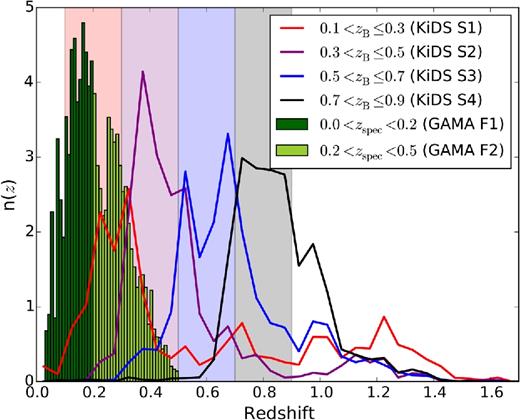
Normalized redshift distribution of the four tomographic source bins of KiDS (solid lines), used to measure the weak gravitational lensing signal, and the normalized redshift distribution of the two spectroscopic samples of GAMA galaxies (histograms), that serve as the foreground sample in the galaxy–galaxy lensing analysis and that are used to determine the angular correlation function. For plotting purposes, the redshift distribution of GAMA galaxies has been multiplied by a factor 0.5. The shaded regions indicate the photometric redshift (zB) selection of the tomographic source bins.
The galaxy shapes were measured from the r-band data using an updated version of the lensfit method (Miller et al. 2013), carefully calibrated to a large suite of image simulations tailored to KiDS (Fenech Conti et al. 2017). The resulting multiplicative bias is of the order of a percent with a statistical uncertainty of less than 0.3 per cent, and is determined in each tomographic bin separately. The additive shape measurement bias is determined separately in each patch on the sky and in each tomographic redshift bin as the weighted average galaxy ellipticity per ellipticity component, and has typical values of ∼10−3. We corrected the additive bias at the catalogue level, while the multiplicative bias was accounted for during the correlation function estimation.
To avoid confirmation bias, the fiducial cosmological analysis of KiDS (Hildebrandt et al. 2017) was blinded: three different shape catalogues were analysed, the original and two copies in which the galaxy ellipticities were modified such that the resulting cosmological constraints would differ. Only after the analysis was written up, an external blinder revealed which catalogue was the correct one. Since the lead authors of this paper were already unblinded elsewhere, the current analysis could no longer be performed blindly. However, since the shear catalogues were not changed after unblinding, we still partly benefit from the original blinding exercise.
We used the KiDS galaxies to measure the cosmic shear correlation functions, and to measure the tangential shear around the foreground galaxies from the GAMA survey (Driver et al. 2009, 2011; Liske et al. 2015). GAMA is a highly complete spectroscopic survey up to a Petrosian r-band magnitude of 19.8. In total, it targeted ∼240 000 galaxies. We use a subset of ∼180 000 galaxies that reside in the three patches of 60 deg2 each near the celestial equator, G09, G12, and G15, as those patches fully overlap with KiDS. The tangential shear measurements in these three patches are combined with equal weighting. Due to the flux limit of the survey, GAMA galaxies have redshifts between 0 and 0.5. We select two GAMA samples, a low-redshift sample with zspec < 0.2, and a high-redshift sample with 0.2 < zspec < 0.5. Their redshift distributions are also shown in Fig. 1.
We also use the same subset of GAMA galaxies to determine the angular correlation function, and thus the corresponding angular power spectrum. To determine the clustering, we make use of the GAMA random catalogue version 0.3, which closely resembles the random catalogue that was used in Farrow et al. (2015) to measure the angular correlation function of GAMA galaxies. We sample the random catalogue such that we have 10 times more random points than real GAMA galaxies.
3.2 Measurements
We use the shape measurement catalogues of KiDS-450 to measure the cosmic shear correlation functions, ξ+ and ξ−, and the tangential shear around GAMA galaxies. All projected real-space correlation functions in this work are measured with treecorr5 (Jarvis, Bernstein & Jain 2004). Since the ξ+ and ξ− measurements have already been presented in Hildebrandt et al. (2017), we will not show them here. The ℓ range in which we can obtain unbiased estimates of the power spectra depends on the angular range where we trust the correlation functions. For ξ+ and ξ−, we use an upper limit of θ < 120 arcmin, as the measurements on larger scales become increasingly sensitive to residual uncertainties on the additive bias correction. The lower limit is 0.06 arcmin, but our power spectrum estimator is insensitive to any signal below 1 arcmin. The PE band powers are nearly unbiased in the range ℓ > 150 (see Appendix A). We measure ξ+ and ξ− in 600 logarithmically spaced bins between 0.06 and 600 arcmin, to account for the rapid oscillations of the window functions used to convert the shear correlation functions to the power spectra, but we only use scales 0.06 < θ < 120 arcmin in the integral.
To test the sensitivity of our estimator to a residual additive shear bias, we also measured the power spectra without applying the additive bias correction. This only affected the lowest ℓ bins by shifting them with a typical amount of 0.5σ; the impact on other bins was negligible. Since the error on the additive bias correction is smaller than the correction itself, its impact on the power spectra is even smaller and can therefore be safely ignored.
Since PE does not vary rapidly with ℓ, we only need a small number of ℓ bins to capture most of the cosmological information. We use five logarithmically spaced bins, whose logarithmic means range from ℓ = 200 to ℓ = 1500; the ℓ ranges they cover can be read off from Fig. A1. Truncating the integral to θ < 120 arcmin leads to a small negative additive bias of the order of 10−6 in the lowest ℓ bin (smaller than the statistical errors). We derive an IBC for this in Appendix A and apply it to all power spectra, although not applying this correction leads to negligible changes of our results. The resulting E modes and B modes are shown in Fig. 2.
Cosmic shear power spectra for KiDS-450, derived with our power spectrum estimator that integrates the shear correlation functions in the range 0.06 < θ < 120 arcmin. The numbers in each panel indicate which shape (S) samples are correlated, with the numbers defined in the legend of Fig. 1. The panels on the left show the E modes, and the ones on the right the B modes. Error bars have been computed analytically. The B modes have been multiplied with ℓ instead of ℓ2 for improved visibility of the error bars. Solid lines correspond to the best-fitting model, for our combined fit to PE, Pgm, and Pgg. There is one ℓ bin whose B mode deviates from zero by more than 3σ, the highest ℓ of the S2–S4 cross-correlation; the corresponding E mode is high as well. We have verified that excluding this bin from the analysis does not change our results.
We obtain a clear detection for PE in each tomographic bin combination. The signal increases with redshift, which is expected as the impact of more structures is imprinted on the galaxy ellipticities if their light traversed more large-scale structure and because of the geometric scaling of the lensing signal (see equation 2).
Fig. 2 also shows PB, the B modes that serve as a systematic test. Note that the IBC has also been applied to the B modes. There are a number of ℓ bins which appear to be affected by B modes; the most prominent feature is the highest ℓ bin for the cross-correlation between the second and fourth tomographic bins. To quantify this, we determined the reduced χ2 value of the null hypothesis for all bins combined, which has a value of 1.96. This corresponds to a p-value of 0.0001. This number is driven by this single ℓ bin; excluding this bin alone lowers the reduced χ2 to 1.55 (and a p-value of 0.0082), which is still a tentative sign of residual B modes. Not applying the IBC slightly improves the overall reduced χ2 to 1.87 (1.45 after removing the suspicious ℓ bin). The origin of the B modes in KiDS is under active investigation and will be presented in Asgari et al. (in preparation). To test how it may affect our cosmological results, we repeat the test of Hildebrandt et al. (2017), subtract the B modes from the E modes, and run the cosmological inference. This B-mode correction shifts our main cosmological result by less than 0.5σ, thus demonstrating that if the source of the B modes also generates E modes in equal amounts, our results are not significantly biased if we do not account for that. More details of this test are provided in Appendix C.
The large amplitude of PB of this suspicious ℓ bin suggests that the corresponding PE measurement might not be trustworthy, and indeed, it appears high. We have tested that removing this single ℓ bin from the analysis does not affect the cosmological inference except for the goodness of fit. Another apparent feature is that the PE of the first ℓ bins of the cross-correlation between the second tomographic bin and the second, third and fourth tomographic bins are ∼2σ below the best-fitting model. However, the first ℓ bins of the various tomographic bin combinations are fairly correlated (see e.g. Fig. B3 in Appendix B2), so this feature is less significant than it appears. Furthermore, in Section 4 we will show that excluding the lowest ℓ bins from the fit does not impact our results.
We have also compared our power spectrum estimates with those derived using the quadratic estimator from Köhlinger et al. (2017). A detailed comparison is presented in Appendix C. Overall, we find good agreement between the E modes, although for one tomographic bin combination we find a noticeable difference at high ℓ. A possible explanation is the presence of some B modes in the cosmic shear correlation functions (as reported in Hildebrandt et al. 2017). This is further supported by the fact that we detect B modes at a higher significance than Köhlinger et al. (2017), where they are found to be consistent with zero. It is still unclear if or how this affects the cosmological inference, although the B-mode correction test we did in Appendix C suggests that the impact is small.
Next, we determined the galaxy-matter power spectrum, for which we needed to measure the tangential shear signal around GAMA galaxies first. This lensing signal is shown in Fig. 3. We also measured the signal with an independent code, and the results agreed very well. For illustrative purposes, we used 20 logarithmically spaced bins between 0.1 and 300 arcmin. To compute the power spectra, we need a much finer sampling, as the window functions used to convert the correlation functions to power spectra oscillate rapidly. Hence we measured the signal in 600 logarithmically spaced bins in the range 0.06 < θ < 600 arcmin, but only used the measurements on scales θ < 120 arcmin to compute the power spectrum.
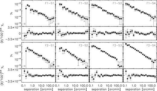
Tangential shear and cross-shear around GAMA galaxies measured with KiDS sources in tomographic bins, as indicated in the panels. The cross-shear measurements have been multiplied with a factor (θ/100)0.5 to ensure that the error bars are visible over the plotted angular range. Open squares show negative points of γt with unaltered error bars. The lensing signal measured around random points has been subtracted, which is consistent with zero on the scales of interest for all but the third tomographic source bin, where it is small but positive on scales >20 arcmin. Furthermore, the signal has been corrected for the contamination of source galaxies that are physically associated with the lenses. The errors are derived from jackknifing over 2.5 × 3 deg non-overlapping patches. They are only used to assess on which scales the signal is consistent with not being affected by systematics; when we fit models to our power spectra we use analytical errors throughout.
Some of the galaxies from the source sample are physically associated with the lenses. They are not lensed and bias the tangential shear measurements. As demonstrated in Mandelbaum et al. (2005), this bias can easily be corrected by multiplying the lensing signal with a boost factor, which contains the overdensity of source galaxies as a function of projected radial distance to the lens. The boost factor generally increases towards smaller separations, but decreases very close to the lens, due to problems with the background estimation caused by the lens light (see e.g. Dvornik et al. 2017). The boost factor can be made smaller by applying redshift cuts to the source sample; here, we do not apply such cuts because we want to use the exact same sources as in the cosmic shear measurements. In our case, the impact of the boost correction is negligible, as our estimator is insensitive to scales θ < 2 arcmin (see Appendix A). At 2 arcmin, the boost factor is 7 per cent at most for the F2–S2 bin, and decreases quickly with radius. For all other bins, the correction is much smaller. We have checked that not applying the boost correction does not significantly affect the power spectra.6
The impact of magnification on the boost factor is negligible in this radial range and can safely be ignored. Furthermore, we measured the tangential shear around random points from the GAMA random catalogue, and subtracted that from the real signal. Apart from removing potential additive systematics in the shape measurement catalogues, this procedure also suppresses sampling variance errors (Singh et al. 2017).
To obtain the errors on our galaxy–galaxy lensing measurements, we split the survey into 24 non-overlapping patches of 2.5 × 3 deg, and used those for a ‘delete one jackknife’ error analysis. These errors should give a fair representation of the true errors, and thus be sufficient to assess at which scales we consider the measurements robust. Note that we used jackknife errors instead of analytical errors on these real-space measurements for convenience; we stress that in the cosmological inference, we used an analytical covariance matrix for all power spectra.
Fig. 3 also shows the cross-shear, the projection of source ellipticities at an angle of 45 deg with respect to the lens–source separation vector. Galaxy–galaxy lensing does not produce a parity violating cross-shear once the signal is azimuthally averaged, and hence it serves as a standard test for the presence of systematics. The cross-shear is consistent with zero on most scales, although some deviations are visible, e.g. at scales of half a degree for the F1–S4 bin. The cross-shear at small separations for the F2–S1 and F2–S2 bins is not worrisome, as our estimator is not sensitive to the galaxy–galaxy lensing signal on those scales. For consistency with the cosmic shear power spectrum, we only use the galaxy–galaxy lensing measurements in the range <120 arcmin. As demonstrated in Appendix A, we can obtain unbiased estimates on Pgm from γt in the range ℓ ≥ 150.
We estimate Pgm using the same ℓ range as for PE/B. The measurements are shown in Fig. 4. We apply the IBC, which on average causes a 6 per cent change in the lowest ℓ bin, and much smaller changes for the higher ℓ bins. We obtain significant detections for all lens–source bin combinations. The error bars have been computed analytically as discussed in Section 3.3. The amplitude of the power spectrum increases for higher source redshift bins as expected, because of the geometric scaling of the lensing signal. We also show Pg ×, the power spectrum computed using the cross-shear, which serves as a systematic test. There are a few neighbouring ℓ bins that are systematically offset, for example the low-ℓ bins of F1–S3 and F1–S4. We already pointed out the presence of some cross-shear in Fig. 3 on the scale of half a degree for those bins, which translates into those Pg × bins. On average, however, the amplitude of Pg × is not worrisome as the reduced χ2 of the null hypothesis has a value of 1.13. The corresponding p-value is 0.27.
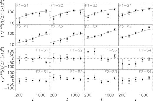
Galaxy-matter power spectrum (top) and galaxy-cross-shear power spectrum (bottom) around GAMA galaxies in two lens redshift bins, measured with KiDS sources using four tomographic source bins. The numbers in each panel indicate the foreground (F) sample–shape (S) sample combination, as defined in Fig. 1. The errors are computed analytically and correspond to the 68 per cent confidence interval. Pg × has been multiplied with ℓ instead of ℓ2 for improved visibility of the error bars. Solid lines correspond to the best-fitting model, for our combined fit to PE, Pgm, and Pgg. The Pg × in the bottom rows serves as a systematic test, and it is consistent with zero.
Finally, to determine Pgg, we first measure the angular correlation function of the two foreground galaxy samples from GAMA. We show the signal in Fig. 5. Errors come from jackknifing over 2.5 × 3 deg patches and only serve as an illustration; in the cosmological inference, we use analytical errors for Pgg. The angular correlation function is robustly measured on all scales depicted. Therefore, we use an upper limit of 240 arcmin in the integral to determine Pgg. We adopt the same ℓ ranges as for PE and Pgm and show the band powers of Pgg in Fig. 6. The angular power spectrum of the F2 sample is lower than that of the F1 sample because the redshift range of F2 is wider. Note that the angular correlation function |$ w $|(θ) has an additive contribution due to the fact that the mean galaxy density is estimated from the same data set. This integral constraint only contributes to the ℓ = 0 mode in Pgg and therefore does not have to be considered further in our modelling.
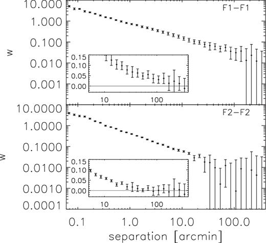
Angular correlation function of the two foreground galaxy samples from GAMA. The inset in each panel shows the signal on large scales with a linear vertical axis. The errors are derived from jackknifing over 2.5 × 3 deg non-overlapping patches and serve for illustration. When we fit models to our power spectra we used analytical errors throughout.
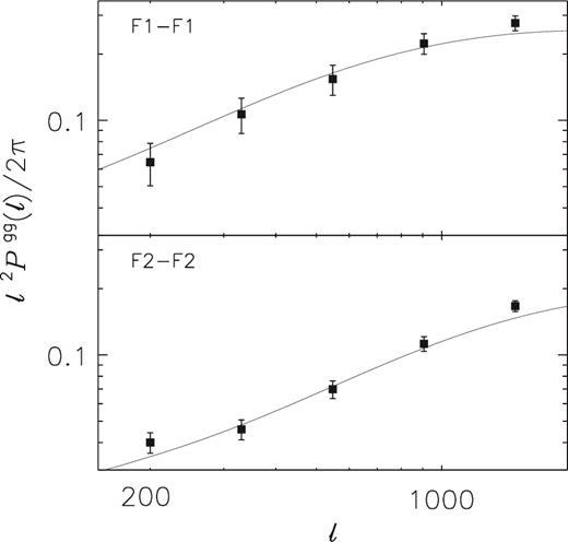
Angular power spectrum of the two foreground galaxy samples from GAMA. The depicted errors are determined analytically. Solid lines correspond to the best-fitting model, for our combined fit to PE, Pgm, and Pgg.
3.3 Covariance matrix
We determine the covariance matrix of the combined set of power spectra analytically, following a similar formalism as in Hildebrandt et al. (2017). The covariance matrix includes the cross-covariance between the different probes. One particular advantage of this approach is that it properly accounts for super-sample covariance (SSC), which are the cosmic variance modes that are larger than the survey window and couple to smaller modes within. This term is typically underestimated when the covariance matrix is estimated from the data itself, for example through jackknifing, or when it is estimated from numerical simulations. Another advantage is that it is free of simulation sampling noise, which could otherwise pose a significant hindrance for joint probe analyses with large data vectors.
The analytical covariance matrix consists of three terms: (i) a Gaussian term that combines the Gaussian contribution to sample variance, shape noise, and a mixed noise-sample variance term, estimated following Joachimi et al. (2008), (ii) an in-survey non-Gaussian term from the connected matter trispectrum, and (iii) a SSC term. To compute the latter two terms, we closely follow the formalism outlined in Takada & Hu (2013), which can be readily expanded to galaxy–galaxy lensing and clustering measurements (e.g. Krause & Eifler 2017).
By subtracting the signal around random points from the galaxy-matter cross-correlation, we effectively normalize fluctuations in the galaxy distribution with respect to the mean galaxy density in the survey area instead of the global mean density. This substantially reduces the response to super-survey modes (Takada & Hu 2013) and diminishes error bars (Singh et al. 2017), and we do account for this effect in our covariance model.
One further complication is that the KiDS survey area is larger than GAMA. While the galaxy-matter power spectrum and the angular power spectrum are measured in the 180 deg2 of the three GAMA patches near the equator that are fully covered by KiDS, the cosmic shear power spectrum is measured on the full 450 deg2 of KiDS-450. This partial sky overlap of the different probes affects the cross-correlation and is accounted for (see Appendix G).
In order to compute the covariance matrix, we need to adopt an initial fiducial cosmology as well as values for the effective galaxy bias. For the fiducial cosmology, we use the best-fitting parameters from Planck Collaboration XIII (2016), and for the effective galaxy biases we assume values of unity for both bins. If our data prefers different values for these parameters, the size of our posteriors could be affected (as illustrated in Eifler, Schneider & Hartlap 2009, for the case of cosmic shear only). Therefore, after the initial cosmological inference, the analytical covariance matrix is updated with the parameter values of the best-fitting model. This is turned into an iterative approach, as detailed in Appendix D. It is made possible by the use of an analytical covariance matrix, which is relatively fast and easy to compute. Since the parameter constraints do not change significantly at the second iteration, we adopt the resulting analytical covariance matrix for all cosmological inferences in this paper.
The analytical covariance matrix for ξ+ and ξ− has been validated against mocks in Hildebrandt et al. (2017). We repeat that exercise for the three power spectra in Appendix B. The analytical covariance matrix agrees well with the one estimated from the N-body simulations. Our choice of power spectrum estimator is not guaranteed to reach the expected errors that we calculate analytically, but the comparison with the simulations did not reveal any evidence for significant excess noise. We did not include intrinsic alignments or baryonic feedback in the covariance modelling, but since all our measurements are dominated by the cosmological signals, the impact of the astrophysical nuisances on sample variance is small.7 We have checked that a potential error on the additive bias correction has a negligible contribution to the covariance matrix.
3.4 Model fitting
To constrain the cosmological parameters, we used cosmomc8 (Lewis & Bridle 2002), which is a fast Markov Chain Monte Carlo code for cosmological parameter estimation. The version we use is based on Joudaki et al. (2017a),9 which includes prescriptions to deal with intrinsic alignment, the effect of baryons on the non-linear power spectrum, and systematic errors in the redshift distribution. This framework has been further developed to simultaneously model the tangential shear signal of a sample of foreground galaxies and redshift space distortions (Joudaki et al. 2018). We extended it by modelling the angular correlation function of the same foreground sample. Furthermore, we modified the code in order to fit the power spectra instead of the correlation functions. Since the conversion from power spectra to correlation functions could be skipped, the runtime decreased by a factor of 2. We computed the power spectra at the logarithmic mean of the band instead of integrating over the band width, as the difference between the two was found to be at the percent level and therefore ignored. We checked that the impact of this simplification on our cosmological parameter constraints was less than 0.3σ for our fiducial data vector.
To model Pgm and Pgg, we assume that the galaxy bias is constant and scale independent. Since we include non-linear scales in our fit, this bias should be interpreted as an effective bias. It is fitted separately for the low-redshift and high-redshift foreground sample. The scale dependence of the bias has been constrained in observations by combining galaxy–galaxy lensing and galaxy clustering measurements for various flux-limited samples and was found to be small (e.g. Hoekstra et al. 2002; Simon et al. 2007; Cacciato et al. 2012; Jullo et al. 2012). In a recent study on data from the Dark Energy Survey, Crocce et al. (2016) constrained the scale dependence of the bias using the clustering signal of flux-limited samples, selected with i < 22.5, modelling the signal with a non-linear power spectrum from Takahashi et al. (2012) with a fixed, linear bias as fit parameter. They report that their linear bias model reproduces their measurements down to a minimum angle of 3 arcmin for their low-redshift samples (although the caveat should be added that our foreground sample is selected with a different apparent magnitude cut). While the aforementioned studies report little scale dependence of the bias in real space, our assumption of a scale-independent bias is made in Fourier space. The largest ℓ bin is centred at 1500, which uses information from ξ+/ − down to scales of less than an arcminute (see Appendix A). Hence a strong scale dependence of the bias on scales less than 3 arcmin could violate our assumption. However, if the bias is strongly scale dependent on scales of ℓ < 1500, this will show up in our measurements as a systematic offset between data and model for the highest ℓ bin of Pgg (and, to a lesser extent, Pgm). Also, on small scales, the cross-correlation coefficient r might differ from one, which would lead to discrepancies between Pgm and Pgg. However, as Figs 4 and 6 show, there is no clear evidence for such a systematic difference, which serves as further evidence that our approach is robust. Also, when we exclude the highest ℓ bin of Pgm and Pgg from our analysis, our results do not change significantly (see Section 4.1).
We validated the Pgg model predictions using an independent code that was internally available to us. The signal agreed to within 3 per cent in the range 150 < ℓ < 2000, with a mean difference of 2 per cent. The small remaining difference is caused by different redshift interpolation schemes of the galaxy number density; in our code, we used a spline interpolation, while a linear interpolation was used in the independent code. When we adopted a spline interpolation in the independent code, the model signal agreed to within 1.5 per cent, with a mean difference of ∼1 per cent. Since it is not a priori clear which interpolation scheme is better, we decided to keep using the spline interpolation scheme. The model prediction of PE has been compared to independent code in Hildebrandt et al. (2017) and was found to agree well. We have not explicitly compared the predictions of Pgm with an independent code, but since that model is built of components used in the computation of Pgg and PE, we expect a similar level of accuracy.
We marginalize over the systematic uncertainty of the redshift distribution of our source bins following the same methodology adopted in Hildebrandt et al. (2017) and Köhlinger et al. (2017), that is by drawing a random realization of the redshift distribution in each step of the MCMC. This approach fully propagates the statistical uncertainties included in the redshift probability distributions, but does not account for sample variance in the spectroscopic calibration data. We investigated the robustness of this method by also fitting models in which we allowed for a constant shift in the redshift distributions. This procedure basically marginalizes over the first moment of the redshift distribution, which is, to first order, what the weak lensing signal is sensitive to Amara & Réfrégier (2007). We discuss the result of this test in Section 4.3. We do not account for the uncertainty of the multiplicative shear calibration correction, as Hildebrandt et al. (2017) showed that it has a negligible impact on correlation function measurements.
To obtain a crude estimate of how much cosmic variance in the source redshift distribution affects our cosmological results, we performed the following test. We used the DIR method separately on the different spectroscopic fields. The variation between the resulting redshift distributions suggests that cosmic variance and Poisson noise contribute roughly equally to the total uncertainty. To estimate the potential impact on our cosmological constraints, we fixed the redshift distribution to the mean from the DIR method, but allowed for a shift in the mean redshift of each tomographic bin, using a Gaussian prior with a width that equals the error on the mean redshift (from table 1 of Hildebrandt et al. 2017). Using this set-up, we recovered practically identical errors on the cosmological parameters compared to our fiducial approach. Next, we increased the width of the Gaussian prior by a generous factor of 1.5, to roughly include the impact of cosmic variance. This increased the error on our cosmology results by 5 per cent. Note that this is a conservative upper limit, as the cosmic variance between the separate spectroscopic fields is larger than the cosmic variance of all the fields combined. Hence we conclude that cosmic variance of the source redshift distribution affects our cosmological constraints by a few per cent at most. We do not adopt this as our fiducial approach, however, since our current method of estimating the impact is not sufficiently accurate.
We adopt top-hat priors on the cosmological parameters, as well as the physical ‘nuisance’ parameters discussed earlier in this section. The prior ranges are listed in Table 1. Furthermore, we fix kpivot, the pivot scale where the scalar spectrum has an amplitude of As, to 0.05 Mpc−1. Even though the sum of the neutrino masses is known to be non-zero, we adopt the same prior as Hildebrandt et al. (2017) and fix it to zero. We have tested that adopting 0.06 eV instead leads to a negligible change in our results. Note that the priors and fiducial values we adopted are the same as in Hildebrandt et al. (2017), which makes a comparison of the results easier. As a test, we also fitted our joint data vector adopting the broader priors on H0 and Ωb from Joudaki et al. (2017b) and found negligible changes to our results, showing that we are not sensitive to the adopted prior ranges of these parameters.
Priors on the fit parameters. Rows 1–6 contain the priors on cosmological parameters, rows 7–10 the priors on astrophysical ‘nuisance’ parameters. All priors are flat within their ranges.
| Parameter | Description | Prior range |
|---|---|---|
| 100θMC | 100 × angular size of sound horizon | [0.5,10] |
| Ωch2 | Cold dark matter density | [0.01,0.99] |
| Ωbh2 | Baryon density | [0.019,0.026] |
| ln (1010As) | Scalar spectrum amplitude | [1.7,5.0] |
| ns | Scalar spectral index | [0.7,1.3] |
| h | Dimensionless Hubble parameter | [0.64,0.82] |
| AIA | Intrinsic alignment amplitude | [ − 6, 6] |
| B | Baryonic feedback amplitude | [2,4] |
| bz1 | Galaxy bias of low-z lens sample | [0.1,5] |
| bz2 | Galaxy bias of high-z lens sample | [0.1,5] |
A number of the assumptions we made could affect the measured or theoretical power spectra, and thus our cosmological constraints, at the per cent level. We have decided to ignore the assumptions whose impact is of the order of 1 per cent or less. This includes the Limber approximation, the flat-sky approximation, and the uncertainty on the multiplicative bias correction. Other effects whose impact is either uncertain or expected to be larger are addressed in the text.
We ran cosmomc with 12 independent chains. To assess whether the chains have converged, we used a Gelman–Rubin test (Gelman & Rubin 1992) with the criterion that the ratio between the variance of any of the fit parameters in a single chain and the variance of that parameter in all chains combined is smaller than 1.03. Furthermore, we have checked that the chains are stable against further exploration. When analysing the chains, we removed the first 30 per cent of the chains as the burn-in phase. Before fitting the measured power spectra from the data, we ran cosmomc on our mock results, and verified that we retrieved the input cosmology. Details of this test can be found in Appendix B3.
4 RESULTS
We fitted all power spectra simultaneously and show the best-fitting model as solid lines in Figs 2, 4, and 6. Overall, the model describes the trends in the data well. The reduced χ2 of the best-fitting model has a value of 1.29 (115.9/[100 data points − 10 fit parameters]) and the p-value is 0.034. Hence our model provides a fair fit. If we exclude the highest ℓ bin of the S2–S4 correlation of PE, whose corresponding B mode is high, the best-fitting reduced χ2 becomes 1.19 without affecting any of the results (a shift of 0.1σ in S8). We do include this particular ℓ bin in all our results below to avoid a posteriori selection.
4.1 Cosmological inference
The main result of this work is the constraint on Ωm–σ8, which is shown in Fig. 7. It is this combination of cosmological parameters to which weak lensing is most sensitive. We recover the familiar ‘banana-shape’ degeneracy between these two parameters, which is expected as gravitational lensing roughly scales as |$\sigma _8^2 \Omega _{\rm m}$| (Jain & Seljak 1997). Also shown are the main fiducial results of KiDS-450 (Hildebrandt et al. 2017) and the constraints from Planck Collaboration XIII (2016). Our confidence regions are somewhat displaced with respect to those of Hildebrandt et al. (2017) and our error on S8 is 28 per cent smaller. Interestingly, our results lie somewhat closer to those of Planck Collaboration XIII (2016), showing better consistency with Planck than KiDS-450 cosmic shear alone. As discussed below, our cosmic shear-only results are fully consistent with the results from Hildebrandt et al. (2017), although not identical, because our power spectra weight the angular scales differently than the correlation functions. Hence this shift towards Planck must either be caused by Pgm or Pgg or a combination of the two.

We computed the marginalized constraint on |$S_8\equiv \sigma _8 \sqrt{\Omega _{\rm m}/0.3}$| and show the results in Fig. 8. The joint constraints for our fiducial setup is |$S_8=0.800_{-0.027}^{+0.029}$|. The fiducial result from KiDS-450 is S8 = 0.745 ± 0.039 (Hildebrandt et al. 2017), whilst those of Planck Collaboration XIII (2016) is S8 = 0.851 ± 0.024.
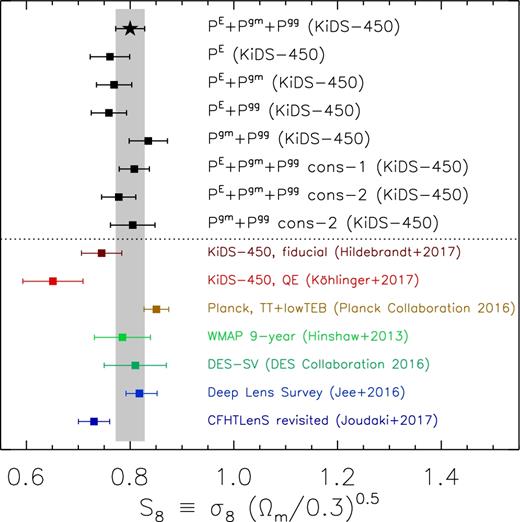
Comparison of our constraints on S8 with a number of recent results from the literature. We show the results for different combinations of power spectra on top with black squares, as well as the results from our conservative runs where we excluded the lowest ℓ bin of all power spectra (cons-1) and the highest ℓ bin of Pgm and Pgg (cons-2) in the fit. In general, our results agree well with those from the literature, including those from Planck.
Compared to the results from Hildebrandt et al. (2017), our posteriors have considerably shrunk along the degeneracy direction. Since we applied the same priors, this improvement is purely due to the gain in information from the additional probes. Hence the real improvement becomes clear when we compare the constraints on Ωm and σ8, for which we find |$\Omega _{\rm m}=0.326_{-0.057}^{+0.048}$| and |$\sigma _8=0.776_{-0.081}^{+0.064}$|, while Hildebrandt et al. (2017) report |$\Omega _{\rm m}=0.250_{-0.103}^{+0.053}$| and |$\sigma _8=0.849_{-0.204}^{+0.120}$|. Hence our constraint on σ8 has improved by roughly a factor of 2 compared to Hildebrandt et al. (2017).10
To understand where the difference between our results and Hildebrandt et al. (2017) comes from, and to learn how much Pgm and Pgg help with constraining cosmological parameters, we also ran our cosmological inference on all pairs of power spectra, as well as on PE alone. The resulting constraints are shown in Fig. 8. Fig. 9 shows the relative difference of the size of the error bars, while Fig. 10 shows the marginalized posterior of Ωm–σ8 and Ωm–S8. Interestingly, the constraints from PE and Pgm + Pgg are somewhat offset, with the latter preferring larger values. The constraint on S8 from PE alone is 0.761 ± 0.038, hence close to the results from Hildebrandt et al. (2017), while for Pgm + Pgg we obtain S8 = 0.835 ± 0.037. PE is only weakly correlated with Pgg and Pgm (see e.g. Fig. B3), and if we ignore this correlation (it is fully accounted for in all our fits), the constraints on S8 from PE and Pgm + Pgg differ by 1.4σ. Since the reduced χ2 is not much worse for the joint fit, our data does not point at a strong tension between the probes, and they can be safely combined.
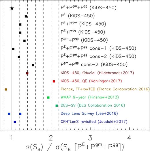
Ratio of the error bar on S8 for various combinations of our data vector and for results from the literature, relative to our fiducial results (PE + Pgm + Pgg). The solid vertical line indicates a ratio of unity, while the dashed lines are displaced by relative shifts of 0.2. Our error bar is 28 per cent smaller than the one from Hildebrandt et al. (2017), while the error bar from Planck Collaboration XIII (2016) is 18 per cent smaller than ours. The two points shown for Jee et al. (2016) are for the quoted lower and upper limit on S8.

Combining PE with Pgm or Pgg results in a relatively minor decrease of the errors of S8 of 11 per cent. Also, the mean value of S8 does not change much. The reason is that the amplitude of Pgm and Pgg, which contains most of the cosmological information, is degenerate with the effective galaxy bias, and as a result, PE drives the cosmological constraints. When both Pgm and Pgg are included in the fit, this degeneracy is broken. Fitting all probes jointly leads therefore to a larger decrease of 26 per cent compared to fitting only PE (see Fig. 9), although this could partly be driven by the displacement of the posteriors in the Ωm–σ8 plane between PE and Pgm + Pgg. Finally, it is interesting to note that PE and Pgm + Pgg have similar statistical power, even though the latter is measured on less than half the survey area (see also Seljak et al. 2005; Mandelbaum et al. 2013). Using the full 3D information content of Pgg instead of the projected quantities that we used here, will improve the cosmological constraining power of this probe even further.
We also performed two conservative runs to test the robustness of our results. In the first run, we excluded the lowest ℓ bins of all power spectra, as it has the largest IBC and our results might be biased if the correction is cosmology dependent. In the second conservative run, we only removed the highest ℓ bins of Pgg and Pgm, as these bins are potentially most biased if the effective galaxy bias (which we assumed to be constant) has some scale dependence, which would affect the small scales (largest ℓ bin) most. The constraints on S8 are also shown in Fig. 8, and the relative increase in errors is shown in Fig. 9. We find fully consistent results. The errors on S8 increase by 4 per cent and 11 per cent for the first and second conservative run, compared to the fiducial results. As a final test, we fitted Pgm + Pgg only excluding the highest ℓ bins. The difference between the constraint on S8 from this run and the fit of PE has decreased to 1.0σ, because of the increase of the error bars and because the results from Pgm + Pgg are shifted to a slightly lower value.
Fig. 8 shows that our results agree fairly well with a number of recent results from the literature. There is a mild discrepancy with the results from Köhlinger et al. (2017), which is noteworthy as they also used the KiDS-450 data set to estimate power spectra, but with a quadratic estimator. The difference is likely caused by a conspiracy of several effects. First of all, Köhlinger et al. (2017) employed a different redshift binning and fitted the signal up to lower values of ℓ, that is in the range 76 < ℓ < 1310; they report in their work that the signal on large scales prefers somewhat smaller values of S8. In Appendix C, we directly compare the power spectrum estimators for the same redshift and ℓ bins. For the highest tomographic bins, the quadratic estimator band powers are lower than our PE estimates at high ℓ. This is accommodated by the model fit of Köhlinger et al. (2017) with a large, negative intrinsic alignment amplitude of AIA = −1.72. Since AIA and S8 are correlated (e.g. see Fig. 12), this pushes the S8 from Köhlinger et al. (2017) down relative to our results. Note that a thorough internal consistency check of KiDS-450 data, including a comparison of the information content from large and small scales, is currently underway (Köhlinger et al. in preparation). A more in-depth discussion of the difference is presented in Appendix C.
The constraints from the other works from the literature that we compare to are consistent with ours (i.e. differences are less than 2σ), as is shown in Fig. 8. This includes the results from Joudaki et al. (2017a), who re-analysed the shear correlation functions from CFHTLenS (Heymans et al. 2013) using the extended version of Cosmomc that we used here as well. Jee et al. (2016) presented results based on a tomographic cosmic shear analysis of the DLS, a deep 20 deg2 survey with a median source redshift of 1.2. Furthermore, we show the first constraints from the DES (Dark Energy Survey Collaboration 2016), who used 139 deg2 of Science Verification data for a tomographic cosmic shear analysis, and finally, we show the results for WMAP9 (Hinshaw et al. 2013). We caution that the above works have been analysed with different models and assumptions, which complicates a detailed comparison of the results.
4.2 Constraints on astrophysical nuisance parameters
Our analysis constrains a number of physical ‘nuisance’ parameters, which are interesting in themselves. Their 1D marginalized posterior means and 68 per cent confidence intervals are shown in Fig. 11, together with the reduced χ2 of the best-fitting model, for all combinations of power spectra as well as for the conservative runs. Overall, we find a fair agreement between the constraints between probes. Interestingly, the fit of PE alone has the worst reduced χ2 of 1.46. However, that fit is relatively more affected by the highest ℓ bin of the S2–S4 cross-correlation, compared to the joint fit; excluding that bin from the fit leads to a reduced χ2 of 1.28, more in line with the χ2 values of the other fits.
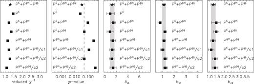
Reduced χ2 values of the best-fitting models, corresponding p-values of the fit, and constraints on the amplitude of the intrinsic alignment model AIA and effective biases of the two foreground samples, bz1 and bz2, for the different combinations of power spectra. The lower points show the results of the conservative run, where we excluded the lowest ℓ bin from PE (c1) and the highest ℓ bin from Pgm and Pgg (c2) in the fit. The red, vertical dashed line in the second panel indicates a p-value of 0.05, the 2σ discrepancy line.
The amplitude of the intrinsic alignment model is well constrained in the combined fit, with AIA = 1.27 ± 0.39. Most of the constraining power on AIA comes from Pgm, as the redshift distributions of the foreground samples and the shape samples partly overlap; fitting only PE, |$A_{\rm IA}=0.92_{-0.60}^{+0.76}$| and is therefore only inconclusively detected. In an analysis of cosmic shear data from CFHTLenS combined with WMAP7 results, Heymans et al. (2013) reported |$A_{\rm IA}=-1.18_{-1.17}^{+0.96}$|. Joudaki et al. (2017a) analysed CFHTLenS data and found AIA = −3.6 ± 1.6, while the correlation function analysis of KiDS (Hildebrandt et al. 2017) reported AIA = 1.10 ± 0.64. Hence, similar to Hildebrandt et al. (2017), our results prefer a positive intrinsic alignment amplitude, but we detect it with a larger significance. The preference for negative values in CFHTLenS but positive values in KiDS suggests that AIA is not simply a measure of the amount of intrinsic alignments of galaxies, but that in fact it accounts for systematic effects that might differ between surveys. Further evidence for this scenario is that the amplitude we obtain is larger than what is expected based on results from previous dedicated intrinsic alignment studies; although intrinsic alignments have been detected for luminous red galaxies (e.g. Joachimi et al. 2011; Singh, Mandelbaum & More 2015), the constraints for less luminous red galaxies and blue galaxies are consistent with zero (Mandelbaum et al. 2006; Hirata et al. 2007; Mandelbaum et al. 2011). We provide evidence that AIA effectively accounts for uncertainty in the redshift distributions in Section 4.3.
The effective biases of the foreground samples are constrained to bz1 = 1.12 ± 0.15 and bz2 = 1.25 ± 0.16 in the combined fit. The most remarkable difference is the lower value for |$b_{\rm z1}=0.78_{-0.18}^{+0.14}$| for PE + Pgm, compared to bz1 = 1.21 ± 0.14 for PE + Pgg, which is a 2.1σ difference. The constraint on the bias, however, is dominated by the angular correlation functions, which is expected as it scales quadratically with the effective bias while the galaxy-matter power spectrum only linearly. A direct comparison of our bias constraints with results from other work is complicated, since most studies focus on volume-limited rather than flux-limited samples, and because the fitting methodology is different. However, values a bit larger than unity are typical for samples selected in luminosity or stellar mass bins close to the mean of our sample (e.g. Zehavi et al. 2011; Zu & Mandelbaum 2015; Crocce et al. 2016). Furthermore, we note that our cosmological results are not sensitive to the actual values of the biases, as the bias is degenerate with the Ωm–σ8 degeneracy, as illustrated in Fig. B5 in Section B3.
The last physical nuisance parameter we fit is the baryonic feedback parameter B. Even when we include Pgm and Pgg in the fit, it is rather poorly constrained at |$B=2.97_{-0.69}^{+0.56}$|. Fitting PE only, we obtain |$B=3.26_{-0.22}^{+0.74}$|, while Hildebrandt et al. (2017) reported |$B=2.88_{-0.88}^{+0.30}$|. All results are consistent with B = 3.13, a pure dark-matter-only model, but the errors are still large and do not rule out that baryonic feedback has some impact on the matter power spectrum (which is supported by observational results on the scaling relation between baryonic properties of haloes and their dark matter content, see e.g. Viola et al. 2015).
The full marginalized 2D posteriors of all fit parameter pairs is shown in Appendix E, and the mean and 68 per cent credible regions of the marginalized 1D posteriors are listed in Table E1.
4.3 Redshift distribution uncertainty
To investigate uncertainty in the redshift distribution, we performed an analysis where we allowed a constant shift in the redshift distributions of our source samples, independently for each tomographic source bin. These shifts a[x]z are defined as nshift(z) = norig(z + a[x]z), with norig and nshift the original and shifted source redshift distribution of tomographic bin [x]. We adopted priors in the range [−0.1, 0.1], as larger shifts are extremely unlikely, given the differences between the various photometric redshift methods tested in Hildebrandt et al. (2017). The purpose of this test is two-fold: it enables us to roughly estimate the impact of unknown systematic uncertainties in the redshift distributions on our results, and it also tests whether our data point to systematic biases in the redshift distributions. The actual redshift bias may be more complicated than a simple shift of the distribution, and future work could explore more complicated redshift bias models, such as changes to the tails of the distribution.
We fit this extended model to our fiducial data set of PE + Pgm + Pgg and to PE only, to test whether they are internally consistent and to assess how much additional constraining power Pgm + Pgg brings. The 2D marginalized posteriors of these four shift parameters, together with those on S8 and the intrinsic alignment amplitude, are shown in Fig. 12. The constraints on the shifts are listed in Table 2. Both data sets clearly prefer a negative offset for the third tomographic bin of ∼−0.05. The joint analysis disfavours a zero shift in this bin at ∼2σ.

Posteriors on the shifts of the redshift distributions of our four tomographic source redshift bins a1z to a4z. Grey dashed lines correspond to our fiducial results where the shifts are fixed to zero.
Mean and 68 per cent credible intervals of the shifts of the four tomographic redshift bins, S8 and AIA.
| Bin shift parameter | PE + Pgm + Pgg | PE |
|---|---|---|
| a1z | |$-0.033_{-0.050}^{+0.030}$| | |$0.008_{-0.041}^{+0.077}$| |
| a2z | |$-0.022_{-0.027}^{+0.030}$| | |$0.018_{-0.036}^{+0.050}$| |
| a3z | |$-0.057_{-0.042}^{+0.012}$| | |$-0.051_{-0.049}^{+0.013}$| |
| a4z | |$0.032_{-0.019}^{+0.068}$| | |$0.039_{-0.017}^{+0.061}$| |
| S8 | |$0.808_{-0.035}^{+0.036}$| | 0.765 ± 0.045 |
| AIA | |$0.89_{-0.58}^{+0.48}$| | |$1.01_{-0.90}^{+1.18}$| |
It has been suggested that the redshift distribution obtained by the DIR method (our fiducial one) and the CC method (a cross-correlation method based on the work of Schmidt et al. 2013; Ménard et al. 2013) are discrepant for this tomographic bin (Efstathiou & Efstathiou, private communication), and fig. 2 of Hildebrandt et al. (2017) indeed indicates that the redshift distribution of the CC method is shifted by roughly this amount towards lower values, relative to the DIR method. A similar shift between the mean of the redshift distributions of DIR and CC is reported in table 1 of Morrison et al. (2017), although this shift is not significant there given that the error on the mean for the CC method is large. Further evidence is presented in appendix A of Joudaki et al. (2017b), who fit for an unknown constant offset of the KiDS-450 shear correlation functions per tomographic bin, and report a weak preference for a negative shift of the third tomographic bin, and finally in Johnson et al. (2017), who cross-correlated galaxies from the 2dFLenS survey with KiDS galaxies using the same photometric redshift bins. For the other tomographic bins, the shifts are consistent with zero. Furthermore, it is interesting to note that including Pgm + Pgg leads to tighter constraints on the shift for the first and second tomographic redshift bin, due to the overlap with the foreground sample.
Allowing for a shift does not significantly change our constraints on S8, as Fig. 12 shows. For the combined data set, we obtain |$S_8=0.808_{-0.035}^{+0.036}$|, entirely consistent with our fiducial |$0.800_{-0.027}^{+0.029}$|. The uncertainty in S8 is 29 per cent larger when we include the redshift shifts in the fit.
We also show the constraints on AIA in Fig. 12. As already alluded to in Section 4.2, AIA may effectively serve as a genuine nuisance parameter, rather than a parameter which corresponds to the actual intrinsic alignment amplitude of galaxies. Allowing for the shifts already leads to weaker constraints centred at lower values, that is |$A_{\rm IA}=0.89_{-0.58}^{+0.48}$| (for the combined fit), but even more interesting is the degeneracy with the shift of the first and second tomographic redshift bin. If the shifts of these two bins are negative, the intrinsic alignment amplitude becomes smaller, which shows that in our fiducial runs, where the shifts are fixed to zero, AIA is at least partly serving as a nuisance parameter that absorbs potential biases in the redshift distributions.
5 CONCLUSIONS
We constrained parameters of a flat ΛCDM model by combining three cosmological probes: the cosmic shear measurements from KiDS-450, the galaxy-matter cross-correlation from KiDS-450 around two foreground samples of GAMA galaxies, and the angular correlation function of the same foreground galaxies. The analysis employed angular band power estimates determined from integrals over the corresponding two-point correlation functions. This simple formalism provides practically unbiased band powers over a considerable range in ℓ. In our case, the range was 150 < ℓ < 2000 (see Appendix A).
We fitted cosmological models to our data using the updated version of the cosmomc pipeline from Joudaki et al. (2017a), extended to simultaneously model galaxy–galaxy lensing measurements (Joudaki et al. 2018). The baseline model consists of a flat ΛCDM model and physically motivated prescriptions for the intrinsic alignment of galaxies and baryonic feedback. We assumed a scale-independent effective galaxy bias for our foreground samples. Fitting this model to the three sets of power spectra simultaneously enabled us to coherently account for the physical nuisance parameters, lifting degeneracies between the fit parameters. We tested our full pipeline on numerical simulations that are tailored to KiDS and recovered the input cosmology.
In the model fitting, we used an analytical covariance matrix, accounting for all cross-correlations between power spectra and also for the partial spatial overlap between KiDS-450 and three equatorial GAMA patches. We validated the analytical covariance matrix with numerical simulations and obtained a reasonable level of agreement. Our approach of using an analytical covariance matrix has the advantage that we can accurately account for the effect of SSC, whose impact is subdominant compared to the other terms but not irrelevant. Furthermore, it enabled us to derive an iterative scheme where we updated the analytical covariance matrix with the best-fitting parameters of the previous run (see Appendix D). This led to a ∼1σ shift of the effective galaxy bias posteriors after one iteration, but the posterior of S8 was not significantly affected (i.e. a shift of less than 0.5σ in the mean).
We obtained tight constraints on the two cosmological parameters to which weak gravitational lensing is most sensitive, Ωm and σ8. Our results can be summarized with the S8 parameter, for which we obtained |$S_8\equiv \sigma _8 \sqrt{\Omega _{\rm m}/0.3}=0.800_{-0.027}^{+0.029}$|. We demonstrated that our three probes are internally consistent, and that including Pgm and Pgg in the fit leads to a 26 per cent improvement in constraining power on S8. We compared our results to a number of recent studies from the literature and found good overall agreement. The fiducial KiDS-450 cosmic shear correlation function analysis (Hildebrandt et al. 2017) revealed a value for S8 that is lower than the Planck cosmology, with the tension being 2.3σ. Interestingly, the results from our combined probe analysis point to a somewhat higher S8 value, in-between the KiDS-450 and Planck results (and consistent with both). Our constraints from cosmic shear alone are fully consistent with the results from Hildebrandt et al. (2017) and maintain the same level of discrepancy with Planck.
The physical nuisance parameters that we marginalize over are interesting in themselves from an astrophysical perspective. However, they have to be interpreted with care. For example, when taken at face value, our constraints on the intrinsic alignment amplitude, AIA = 1.27 ± 0.39, suggests that galaxies are on average intrinsically aligned with the large-scale density field. However, by allowing for an additional shift in the source redshift distributions in the fit, we demonstrated that AIA could partly work as a nuisance parameter that accounts for such residual biases in the redshift distributions. This test also demonstrated that our data prefers a small, negative shift of the redshift distribution of the third bin with |$\Delta z=-0.057_{-0.042}^{+0.012}$|, but this does not impact our cosmological results. The nuisance parameters are better constrained when Pgm and Pgg are included in the fit, which highlights the power of combining these cosmological probes. Marginalizing over wide priors on the mean of the tomographic redshift distributions yields consistent results for S8 with an increase of |$28\, {per \,cent}$| in the error.
As in Hildebrandt et al. (2017), we detect B modes in the cosmic shear signal at a low level. Under the strong assumption that the underlying residual systematic generates the same amount of E and B modes, we obtain a 0.5σ shift in S8 away from the Planck values. As the cause of the systematic is currently unknown, we caution that its eventual correction could lead to similar changes in the S8 posterior.
Another KiDS study of a similar nature has run in parallel to this work and will be presented imminently in Joudaki et al. (2018) In that work, cosmic shear measurements from KiDS-450 are combined with galaxy–galaxy lensing and redshift space distortion measurements for a foreground sample of galaxies from BOSS (Dawson et al. 2013) and 2dFLenS (Blake et al. 2016). Even though the analyses differ in many aspects (e.g. different lens samples, different clustering statistics, different scales used in the fit, different methods to estimate the covariance matrices and different priors in the fit), the combination of probes used in that work lead to a similar |${\sim } 20\, {per \,cent}$| decrease of the error bar of S8, but maintain in tension with Planck.
Our work shows that large-scale structure self-calibration methods work on real data. This not only leads to significant improvements in the constraints of cosmological parameters, but also properly accounts for nuisance effects such as galaxy bias, intrinsic alignments, and biases in the source redshift distributions. Future extensions of this work will include other cosmological probes such as redshift space distortions, but also explore extensions of the astrophysical and cosmological models considered.
Acknowledgements
We thank Elisabeth Krause for a helpful comparison of covariance models, Hiranya Peiris for useful discussions, and Andy Taylor, Niall MacCrann, and Gerrit Schellenberger for useful feedback on the draft. We thank our referee, Joe Zuntz, for valuable feedback. EvU and BJ acknowledge support from an STFC Ernest Rutherford Research Grant, grant reference ST/L00285X/1. BJ acknowledges support by an STFC Ernest Rutherford Fellowship, grant reference ST/J004421/1. JHD acknowledges support from the European Commission under a Marie-Sklodwoska-Curie European Fellowship (EU project 656869). CH and MA acknowledge support from the European Research Council under grant number 647112. CB acknowledges the support of the Australian Research Council through the award of a Future Fellowship. Parts of this research were conducted by the Australian Research Council Centre of Excellence for All-sky Astrophysics (CAASTRO), through project number CE110001020. HH is supported by an Emmy Noether grant (No. Hi 1495/2-1) of the Deutsche Forschungsgemeinschaft. This work was supported by the World Premier International Research Center Initiative (WPI), MEXT, Japan. TDK is supported by a Royal Society URF. This work is supported by the Deutsche Forschungsgemeinschaft in the framework of the TR33 ‘The Dark Universe’. KK acknowledges support by the Alexander von Humboldt Foundation. The research leading to these results has received funding from the People Programme (Marie Curie Actions) of the European Union’s Seventh Framework Programme (FP7/2007-2013) under REA grant agreement number 627288. RN acknowledges support from the German Federal Ministry for Economic Affairs and Energy (BMWi) provided via DLR under project no. 50QE1103. MV acknowledges support from the European Research Council under FP7 grant number 279396 and the Netherlands Organisation for Scientific Research (NWO) through grants 614.001.103. This work is based on data products from observations made with ESO Telescopes at the La Silla Paranal Observatory under programme IDs 177.A-3016, 177.A-3017, and 177.A-3018. GAMA is a joint European-Australasian project based around a spectroscopic campaign using the Anglo-Australian Telescope. The GAMA input catalogue is based on data taken from the Sloan Digital Sky Survey and the UKIRT Infrared Deep Sky Survey. Complementary imaging of the GAMA regions is being obtained by a number of independent survey programs including GALEX MIS, VST KiDS, VISTA VIKING, WISE, Herschel-ATLAS, GMRT, and ASKAP providing UV to radio coverage. GAMA is funded by the STFC (UK), the ARC (Australia), the AAO, and the participating institutions. The GAMA website is http://www.gama-survey.org/.
Author Contributions: All authors contributed to the development and writing of this paper. The authorship list is given in three groups: the lead authors (EvU, BJ, SJ), followed by two alphabetical groups. The first alphabetical group includes those who are key contributors to both the scientific analysis and the data products. The second group covers those who have either made a significant contribution to the data products, or to the scientific analysis.
Footnotes
The boost correction implicitly assumes that satellite galaxies are not intrinsically aligned with the foreground galaxies, although our model can account for such alignments. Most dedicated studies of this type of alignments show that it is consistent with zero (see e.g. Sifón et al. 2015, and references therein). If it is not, this could incur a small bias in the boost correction. We will address this in a future work.
By far the most strongly affected bin combination is F2–S1 whose redshift distributions have substantial overlap. For AIA = 1, the galaxy position-intrinsic shape correlation contributes at most 17 per cent to the total signal, with little dependence on angular scale.
The improvement compared to the PE only results that are discussed below is ∼44 per cent.
REFERENCES
APPENDIX A: ACCURACY OF THE POWER SPECTRUM ESTIMATORS
By definition, our power spectrum estimators from equations (5), (11), and (17) are unbiased when we integrate the corresponding real-space correlation functions from zero to infinity. However, even if the correlation functions are measured over a finite range, we can extract practically unbiased band powers over a considerable range in ℓ. Outside this range, the measured power spectra can be corrected for this integral bias. We show that this correction is robust, but recommend only applying it when the bias correction is smaller than the statistical errors, as is the case here.
For this test, we compute the 3D matter power spectrum with the non-linear corrections from Takahashi et al. (2012) and the transfer function fit by Eisenstein & Hu (1998), adopting cosmological parameters that correspond to the best-fitting values of Planck Collaboration XIII (2016). We convert this into the convergence power spectrum using the redshift distribution of our fourth tomographic bin, which has the highest signal-to-noise and is therefore the most conservative test case. This is then converted into the shear correlation functions ξ+/ − using equation (3), adopting the same θ binning as on the data. These are treated as the observed correlation functions, and inserted in equation (5) and (8) to estimate PE and PB, respectively, using the same ℓ ranges that we adopted in the data.
In the first column on Fig. A1, we show how the recovered band powers vary when we increase the lower limit of the integrals of equation (5). Each row corresponds to a given ℓ range, as indicated in each panel. The solid black line is the recovered band power, while the dashed red line corresponds to the theoretical power spectrum at the logarithmic mean of the ℓ bin. The band powers become biased when the lower limit of the integral becomes larger than 1 arcmin. The higher ℓ bins are more strongly affected, as expected, as they retrieve more information from small angular scales. The cyan area indicates the analytical error on PE for the fourth tomographic bin of KiDS-450. Since we can measure the shear correlation functions to much smaller scales than 1 arcmin, we conclude that our band powers are not biased from shifting the minimum scale from zero to 0.06 arcmin.
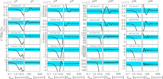
Recovered band powers from analytically computed real-space correlation functions, obtained by varying the lower limit of the conversion integral whilst keeping the upper limit fixed to 600 arcmin (the first, third, fifth, and seventh column), or by varying the upper limit whilst keeping the lower limit fixed to 0.06 arcmin (the second, fourth, sixth, and eighth column). The black line indicates the recovered power spectrum, the red line the input power spectrum at the logarithmic mean of the ℓ bin. The five rows correspond to five different ℓ ranges, indicated in the panels. The first two columns are for PE, column 3–4 for PB, column 5–6 for Pgm, and column 7–8 for Pgg. We use the lens and source redshift distributions from the data, and select those bins that have the highest signal to noise. For PE/B, that is the S4–S4 bin, for Pgm it is F2–S4, and for Pgg it is F2–F2. Other bins show similar trends. The cyan regions indicate the analytical error for those bins in our data. The thin dotted vertical lines show the maximum scales available in the data (2 deg for PE and Pgm, 4 deg for Pgg), showing that the lowest ℓ bin may suffer from a small bias, which we correct for.
In the second column, we repeat the exercise, but now changing the upper limit of the integral. The highest ℓ bins are completely unaffected. The band powers in the lower ℓ bin become biased if the upper limit becomes less than 200 arcmin. We measure the shear correlation functions in the data up to 120 arcmin. For that scale, there is a small bias for the lowest ℓ bin, but it is smaller than our statistical error. We apply an IBC by adding the difference between the observed and input power spectrum, to the one measured on the data. A similar correction scheme was implemented for a power spectrum estimator in Tröster et al. (2017) in the context of a cross-correlation study of gamma-ray maps with weak lensing data.
The third and fourth columns show the corresponding B modes. The trends are similar as for PE: we recover B modes in the range where the E modes are biased. However, if there are significant B modes in the data, it does not automatically mean that they are caused by leakage in our band power estimators. If leakage is present, it is most likely to affect the first and the last ℓ bin.
The fifth and sixth column show the results for the galaxy-matter power spectrum. The analytical power spectra are determined with equation (10), where we used the redshift distribution of the F2 foreground sample from GAMA, adopted an effective bias of unity, and used the redshift distribution of the fourth tomographic shape sample from KiDS-450 to estimate the lensing efficiencies. We recover a similar result. Given the ℓ ranges, our band powers are unbiased as long as we use a minimum lower limit of 2 arcmin or less, which is trivially met. Furthermore, for a maximum scale of 120 arcmin (the maximum scale available in the data), there is a small bias in the lowest ℓ bin, which we correct for.
The final two columns repeat this test for the angular power spectrum. The angular power spectrum is more sensitive to the lower limit of the integral, and the highest ℓ bin becomes significantly biased if the minimum scale is less than 0.2 arcmin; we measure the angular correlation function up to 0.06 arcmin in the data, hence the highest ℓ bin is not affected by the integral bias. The lowest ℓ bin is recovered without bias as long as the maximum scale is 200 arcmin or more. Since we trust the angular correlation function up to 4 deg, also this bin should not be biased. The larger sensitivity to the lower limit of the integral comes from the mixing between θ and ℓ scales through J0. PE, for example, uses information from both ξ+ and ξ−, which yields a different mixing between θ and ℓ scales through the combination of J0 (for ξ+) and J4 (for ξ−). If we adopt K+ = 1 to compute PE (i.e. only using information from ξ+), the bias increases much faster when the lower limit of the integral increases, similar to what is observed for Pgg.
Note that in Fig. A1, we chose the combinations of foreground sample and shape sample bins that resulted in the highest signal-to-noise, which are the most affected by the integral bias. We have checked that the relative impact of the integral bias is smaller for the other power spectra, relative to their statistical powers.
We computed the IBC for all power spectra and applied it to the data. We note that applying this correction has a negligible effect on our results; the constraints on S8 shift by less than 0.2σ if we do not apply the correction. The error on the IBC correction will therefore cause a shift of S8 that is much smaller than 0.2σ.
To test the dependence of the IBC on cosmology, we repeated the test for a Planck cosmology where we either increased or decreased the value of σ8 by 10 per cent. As a result, the curves shown in Fig. A1 shifted vertically, meaning that the error on the IBC linearly depends on the error of the amplitude of the theoretical power spectrum used to compute the correction. It is unlikely that the amplitude of the theoretical power spectrum is off by more than 10 per cent, which puts an upper limit on the bias of the IBC of ∼10 per cent as well. As long as the IBC is smaller than the measurement errors, such an error is subdominant and will not impact the results. Second-order effects, such as small differences in the shape of the power spectrum, are expected to lead to even smaller biases. We note that the issue of a cosmology dependence of the IBC can be circumvented by computing a new correction for every cosmological model evaluated in the MCMC and applying that to the data before determining the likelihood.
APPENDIX B: VALIDATION ON MOCKS
Next, we determine the accuracy of our power spectrum estimators on numerical simulations, which enables us to test whether we measure the correlation functions correctly, and whether the redshift distributions are properly accounted for. The main purpose of these numerical simulations, however, is to compute the covariance matrix from different realizations in order to validate the analytical covariance matrix, and secondly, to test our cosmological inference pipeline by fitting the mock power spectra (using the analytical covariance matrix, hence mimicking the observational procedure), to verify whether we recover the input cosmology.
The mock catalogues are based on the Scinet Light Cone Simulations ( Harnois-Déraps & van Waerbeke 2015), a series of about 1000 N-body simulations tailored for weak lensing surveys. Each realization follows the evolution of 15363 dark matter particles in a cube that measures 505 Mpc h−1 on a side, which are projected on 18 redshift mass planes in the range 0 < z < 3. Light cones are then extracted from these planes on 77452 pixel grids and turned into convergence and shear maps by ray-tracing. The cosmology is fixed to WMAP9 + SN + BAO, 11 that is Ωm = 0.2905, ΩΛ = 0.7095, Ωb = 0.0473, h = 0.6898, σ8 = 0.826 and ns = 0.969.
These mocks have been tailored specifically for the KiDS-450 analyses and were first presented in Hildebrandt et al. (2017), although the version we use here has a larger opening angle (100 deg2 instead of 60 deg2). Source galaxies are placed at random positions in the mocks and are assigned both a true redshift (enforcing the tomographic n(z) estimated with the DIR method, see Hildebrandt et al. 2017) and a photometric redshift, zB, based on the joint probability distribution of these two quantities. This enables the selection of tomographic redshift bins whose true redshift distributions exactly match those of KiDS. The gravitational shears are interpolated from the simulated shear maps at the galaxy positions, while the intrinsic ellipticities are from a Gaussian with a width equalling the intrinsic ellipticity dispersion measured for KiDS galaxies.
To simulate a foreground galaxy sample, which we need to measure the galaxy-matter power spectrum and the angular power spectrum, we use the simulation boxes that are at a mean redshift of z = 0.221 and span a redshift range of 0.1747 to 0.2680. Lens positions are drawn from the projected mass maps with a probability that is proportional to the density, ensuring that the bias of the lens sample is constant at b = 1 and does not depend on scale. Having a lens sample with a known bias is advantageous as we can check whether we recover it. The disadvantage is that it does not enable us to test whether the effective galaxy bias is scale independent in the simulations. Although our mock foreground sample does not reproduce the galaxy sample from GAMA, it allows us to test our pipelines by replacing the GAMA clustering and redshift distribution by that of these mock foreground galaxies.
For simplicity, we only use one lens sample and two source samples, selected with 0.1 < zB ≤ 0.5 and 0.5 < zB ≤ 0.9, respectively. The various real-space correlation functions are measured with the same pipelines as those applied to the data, and converted into power spectra using the same angular scales.
B1 Validating the power spectrum estimator
We measured the cosmic shear correlation functions of our two source samples (two autocorrelations and one cross-correlation), the two tangential shear signals around the foreground sample, and the clustering signal of the foreground sample, and converted those into their respective power spectra, using the same angular ranges that we adopted in the data. We compare that to theoretical predictions, computed for the same cosmological parameters that were used in the mocks and using the non-linear corrections of either Smith et al. (2003) or Takahashi et al. (2012). These theoretical power spectra bracket the power spectrum measured directly from the simulations (see Harnois-Déraps & van Waerbeke 2015).
The ratio of the power spectra measured on the mocks and the theoretical power spectra is shown in Fig. B1. The theoretical power spectra computed using Smith et al. (2003) are up to 10 per cent smaller than the power spectra measured on the mocks, while the theoretical predictions using Takahashi et al. (2012) agree very well, and only overestimate the signal by ∼5 per cent of the cosmic shear S2–S2 power spectrum. If the mock power spectra lie right in the middle of the Smith et al. (2003) and Takahashi et al. (2012) predictions (as was found in Harnois-Déraps & van Waerbeke 2015), we conclude that our power spectra are accurate to better than ∼5 per cent. This is the relative precision with respect to the simulations, not the absolute precision of our estimator. As demonstrated in Appendix A, the absolute error of our estimator is much smaller than the statistical errors and can therefore be safely ignored in our error budget.

Ratio of power spectra measured on the numerical simulations and the theoretical power spectra. The top row shows the autocorrelation and cross-correlation of the cosmic shear power spectra for the two shape samples, the middle row shows the galaxy-matter power spectrum for one foreground sample and two shape samples, and the bottom row shows the angular power spectrum of the foreground sample. Open black circles (blue triangles) correspond to theoretical power spectra computed using the non-linear corrections of Smith et al. (2003) (Takahashi et al. 2012). Error bars show the error on the mean of the different mock realizations.
Note that the tangential shear signal around the foreground sample steeply drops on scales <2 arcmin, which is a sign that their positions do not exactly coincide with the centre of their dark matter haloes. This may be due to the finite resolution of the simulations. However, as Fig. A1 shows, this does not affect Pgm, as the band power in the highest ℓ bin only becomes biased if the lower limit of the integral is larger than 3 arcmin.
B2 Validating the covariance matrix
We computed the covariance matrix of the numerical power spectra using 136 different realizations of the mocks. We do this separately using galaxy shapes with and without intrinsic shape noise. We consider the case without shape noise as it enables us to assess whether the non-Gaussian in-survey term and the SSC term, which are subdominant in the presence of shape noise, are correctly modelled.
We computed the analytical covariance matrix using the specifics of the mocks, that is with the same cosmological parameters, the same mock foreground and source redshift distributions, the same mock intrinsic shear dispersion, and the same mock survey coverage (a total survey area of 100 deg2, with complete overlap between the three probes).
A comparison of the covariance matrix for the mocks without shape noise is shown in Fig. B2. The left-hand panel shows the ratio of the square root of the diagonals, while the right-hand panel compares the off-diagonal terms. In the left-hand panel, we compare to analytical covariance matrices with and without a SSC contribution. The mocks have some SSC from the regions in the original simulation boxes that were outside the light cones, but not the full effect, hence we expect the two analytical predictions to bracket the result from the numerical simulations, which they do for the cosmic shear power spectra. For Pgm and Pgg, the analytical error is ∼10 per cent smaller than the error estimated from the mocks.
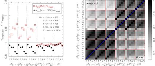
Comparison of the analytical and numerical simulation covariance matrix, for the case without shape noise. The left-hand side shows the ratio of the square root of the diagonals, separately for the six different power spectra. Numbers on the horizontal axis correspond to the different ℓ ranges, as indicated in the figure. Red open squares correspond to the full analytical covariance matrix, black circles to the analytical predictions excluding SSC. These two extremes bracket the mock covariance, which has some SSC, but not the full effect. The right-hand side shows the correlation matrix, with the analytical covariance including SSC in the top left and the numerical simulation covariance matrix in the lower right. The off-diagonal terms agree reasonably well.
In the right-hand panel, we compare the off-diagonal terms of the mock covariance to the analytical one including SSC. We find a good overall agreement, suggesting that the cross-correlation of the different power spectra is correctly modelled with our analytical covariance matrix. The mean difference of the off-diagonal elements of the analytical and mock correlation matrix is only ∼0.06.
In Fig. B3, we repeat the test for the case with shape noise. The left-hand panel shows that the analytical covariance with and without SSC is quite similar, because the covariance matrix is dominated by shape noise. We find a good overall agreement between the diagonals, with typical differences of the order of 10 per cent for the three power spectra. Given the small residual differences in the power spectra measurements, this level of agreement is expected. Also the off-diagonal terms match well. The covariance between the different power spectra is much smaller, and there is little correlation left between PE and Pgm or Pgg.
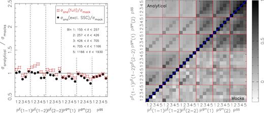
Similar to Fig. B2, but with the inclusion of shape noise.
B3 Validating the cosmological inference
The final purpose of the mocks is to test our cosmological inference pipeline. We fit different combinations of mock power spectra, using the analytical covariance matrix that includes SSC. The mocks have an area of 100 deg2, which is smaller than the survey area of the data. To ensure that the cosmological inference is unbiased given our current statistical precision on the data, we simply rescale the analytical covariance matrix such that it corresponds to an area of 500 deg2. Consequently, the SSC contribution to the analytical covariance matrix is not completely correctly modelled, but since its impact is relatively small it is not expected to affect our results much.
We use the extended version of cosmomc using the same settings as on the data and with the same convergence criterion. The resulting constraints on Ωm–σ8 are shown in Fig. B4. The input cosmology is indicated with the grey cross-hair and falls comfortably within the 1σ contours for all combinations of power spectra that we fit. Hence our cosmological inference pipeline correctly retrieves the input parameters of the mocks, and any remaining systematic bias is smaller than our statistical precision. The constraints from the various power spectrum combinations show little scatter, since we fit the mean signal of the different realizations of the mocks.
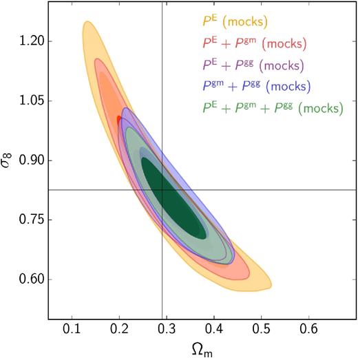
Constraints on Ωm–σ8 for different combinations of mock power spectra, measured on the numerical simulations, assuming a total effective survey area of 500 deg2. The cross-hair indicates the input cosmology, which is comfortably recovered by our fitting pipeline.
In all fits, the bias of the foreground sample is consistent with unity, the input value (except when we only fit PE, which leaves b unconstrained), although for PE + Pgg + Pgm it is shifted by 0.3σ towards lower values. This explains why the cross-hair in Fig. B4 is not exactly centred in the middle of the contours for this power spectra combination. If we fix the bias to unity, the contours shrink dramatically and centre on the cross-hair. The degeneracy between the bias and the degeneracy direction of the posterior in the Ωm–σ8 plane is further illustrated in Fig. B5, where we colour-coded the posterior of the PE + Pgg + Pgm fit using the average values of the bias.
Constraints on Ωm–σ8 obtained by fitting all mock power spectra simultaneously, colour-coded by the value of the bias. It illustrates the degeneracy between the bias and the Ωm–σ8 degeneracy. The cross-hair indicates the input cosmology, at which point the bias has a value of unity.
Ideally, one would like to know whether our estimators are unbiased for a much larger survey (e.g. 10 times larger than KiDS). However, we already noted in Section B1 that we do not exactly recover the input power spectra, but that there are differences left of up to ∼5 per cent. It is unclear whether these differences are caused by limitations of our mocks, of our analytical predictions or of our power spectra estimators, although we note that the tests on the analytical power spectrum–correlation function pairs in Appendix A, as well as tests we have performed on Gaussian random fields (not reported here), suggest that the accuracy of our power spectrum estimator is much better than 5 per cent. For future surveys with improved statistical power, these tests need to be revisited to a higher level of precision.
APPENDIX C: COMPARISON TO QUADRATIC ESTIMATOR
We compare our band powers to the quadratic estimator from Köhlinger et al. (2017). To do that, we adopt the redshift binning from that work, that is three tomographic source redshift bins selected with SK1 = 0.1 < zB ≤ 0.3, SK2 = 0.3 < zB ≤ 0.6 and SK3 = 0.6 < zB ≤ 0.9. We measure the shear correlation functions with our standard angular binning, apply the shear calibration bias corrections, and estimate our power spectra for the same ℓ binning as Köhlinger et al. (2017). Note that we use the full KiDS-450 area to measure the shear correlation functions, while Köhlinger et al. (2017) exclude 36 deg2 from disconnected patches. We have tested that excluding those fields does not affect our measurements. Furthermore, we do not apply an IBC to our band powers, which means that our first ℓ bin is biased low. These limitations should not affect the comparison much. The results are shown in Fig. C1. We plot the full statistical error bars in both cases. The differences between the power estimates should be substantially smaller than these errors as the input data is practically identical, although residual fluctuations will occur because the measurements are weighted differently in the quadratic and band power estimates.
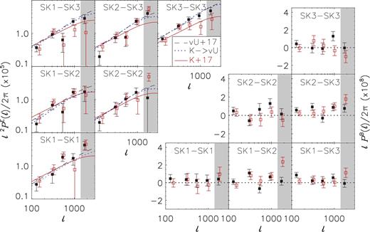
Comparison of PE (left-hand panels) and PB (right-hand panels) for the various tomographic bin combinations, measured with our estimator (black, solid squares) and the quadratic estimator from Köhlinger et al. (2017) (red, open squares). The black dashed lines indicate the best-fitting model from PE alone from this work, the dotted blue line indicates the best-fitting model to PE using the cosmological inference code from Köhlinger et al. (2017), and the solid red lines indicate the best-fitting model from Köhlinger et al. (2017). The measurements in the grey area were excluded from the cosmological inferences with the Köhlinger et al. (2017) model. The only noticeable difference between the estimators is observed for the highest tomographic bin of PE, where our estimator returns higher band powers at large ℓ than the quadratic estimator.
We find a fair agreement for PE for the first and second tomographic bin. For the third tomographic bin, our band powers at high ℓ are higher than the quadratic estimator. This is most apparent in the SK3–SK3 bin. The B modes also appear to show fair agreement, except for the highest ℓ bin in the SK3-SK3 combination and in the SK2-SK3 combination, where again the band powers are higher than the power determined from the quadratic estimator. We note that both estimators were tested on very similar (B-mode free) Gaussian random field simulations and found to faithfully reproduce the input power, which implies that the differences seen are due to some systematic trend in the data that was not included in the mocks. A corresponding trend can be seen in fig. D11 of Hildebrandt et al. (2017). In their autocorrelation of the third tomographic bin (which has substantial overlap with SK3), ξB displays a positive signal below ∼4 arcmin. While our band power estimator is sensitive to these scales in the correlation function, the quadratic estimator is expected to be immune to systematics at a few arcminutes or less. Note that we find similar reduced χ2 values of the null-hypothesis as for our fiducial four redshift bin analysis, while Köhlinger et al. (2017) report that their B modes are consistent with zero.
To test for the potential impact of B modes on the cosmological inference, Hildebrandt et al. (2017) applied a correction under the assumption that the underlying systematics contribute equally to the E- and B modes, which led to a downward shift in S8 by ∼1 σ, in the direction of the Köhlinger et al. (2017) results. We repeated this test by creating a new data vector where we subtracted the B modes from the E modes. We updated the covariance matrix by adding the analytical B-mode covariance matrix to the E-mode one. The cosmological inference resulted in S8 = 0.787 ± 0.034, which is within 0.5σ of our fiducial result. As in Hildebrandt et al. (2017), the shift is towards the results from Köhlinger et al. (2017), but does not close the gap. As the source of the low-level B-mode contamination is currently unknown (see the discussion in Hildebrandt et al. 2017), we do not know how it affects the E modes, hence we do not attempt to remove it in our fiducial analysis but defer this to forthcoming work. It is interesting to note that the B-mode signature appears to vary with the choice of redshift binning (cf. Figs C1 and 2). The link between cosmic shear B modes and binning in terms of a photometric redshift point estimate will be explored in more detail in Asgari et al. (in preparation).
Fig. C1 also shows the best-fitting model from Köhlinger et al. (2017), our best-fitting model from fitting PE only on the default KiDS-450 four-bin data (but shown for the current three tomographic redshift bins), as well as the best-fitting model obtained by applying the cosmological inference method of Köhlinger et al. (2017) to our band powers. The differences between the latter two are small, which suggests that differences in modelling choices are not driving the shift of S8; these include the approaches to the non-linear matter power spectrum, baryon feedback and massive neutrinos, which might contribute at a lower level. The lower quadratic estimator band powers at high ℓ for the SK3–SK3 bin is accommodated by the model with a negative intrinsic alignment amplitude, AIA = −1.72 (weighted median), albeit with large error bars. The fit of the Köhlinger et al. (2017) to our band powers results in an intrinsic alignment amplitude of AIA = 1.53. Since AIA is correlated with S8 (see Fig. 12), this lowers the constraints on S8 from Köhlinger et al. (2017) relative to our results. Such a large, negative intrinsic alignment amplitude is not expected from physical models of the effect. Given the findings of Section 4.3, the low value of AIA could point to inconsistencies in the relative strengths of the tomographic power spectra caused by biases in the redshift distributions.
APPENDIX D: ITERATED ANALYTICAL COVARIANCE MATRIX
In our first run on the data, we used an analytical covariance matrix computed using the best-fitting parameters of Planck Collaboration XIII (2016), and effective galaxy biases of unity for the two foreground samples. If the parameter values we adopted for the covariance model were far from the high-probability region in the resulting posterior, our inferred cosmological model would be inconsistent with the error model used in the likelihood. For example, if we underestimated the effective galaxy biases, the error bars on Pgm and Pgg would be too small and these power spectra would get too much weight in the cosmological inference. Therefore, we updated the analytical covariance matrix using the best-fitting parameters from our initial fit to the data, and repeated the cosmological inference. We repeated this procedure a second time to make sure that this iterative approach is stable and converging. Ideally, one would like to update the analytical covariance matrix in each step in the chain during the cosmological inference, but the computational demands make this approach currently infeasible. Note that in these runs, we did not marginalize over the uncertainty of the source redshift distributions, as we found that to be less stable due to the increased noise.
In Fig. D1, we show the reduced χ2 of the best-fitting model, the constraints on S8 and on the nuisance parameters bz1 and bz2 in each step of the iteration. The reduced χ2 of the initial fit is 1.34 and remains constant. The constraints on S8 does not change much either and is therefore not sensitive to small changes in the parameters of the analytical covariance matrix. The effective biases, however, change significantly. The constraints from the initial fit are bz1 = 1.25 ± 0.13 and bz2 = 1.43 ± 0.15, while the constraints after the second iteration are bz1 = 1.11 ± 0.15 and bz2 = 1.25 ± 0.17. Hence the posteriors shift not only by about 1σ, but also the 68 per cent confidence intervals increase. The cosmological parameters that are degenerate with the galaxy biases, in particular Ωm and σ8, shifted by similar amounts. All cosmological inferences on data in this paper use the analytical covariance matrix based on the best-fitting parameters of the second iteration, as the parameters do not change significantly after another iteration.
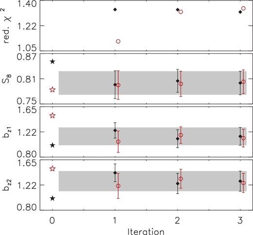
Constraints on the reduced χ2 value of the best-fitting model and the fit parameters S8, bz1 and bz2, where we iteratively update the analytical covariance matrix using the best-fitting parameter values from the previous run, and starting with a fiducial Planck Collaboration XIII (2016) cosmology and effective galaxy biases of unity (black stars) or starting with a fiducial WMAP9 cosmology and effective galaxy biases of 1.5 (red stars). The subsequent constraints are shown by black diamonds and red circles for the Planck and WMAP9 runs, respectively. The constraints on the galaxy biases shift significantly after the first iteration, but do not change after the second iteration.
To test the stability of this iterative procedure, we also computed the analytical covariance matrix using a WMAP9 cosmology (Hinshaw et al. 2013) and effective galaxy biases of 1.5 and used that as the starting point. The resulting parameter constraints are also shown in Fig. D1. The results converge after the first iteration and are thus not very sensitive to the exact starting point of the iterative procedure.
APPENDIX E: FULL POSTERIOR
We show the full posterior of all fit parameters in our fiducial run in Fig. E1, which highlights the degeneracies between parameters. The mean and 68 per cent confidence interval of the fit parameters for the different combinations of power spectra are listed in Table E1.
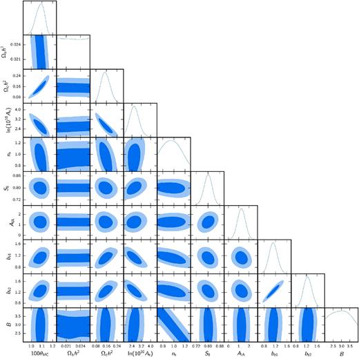
Posterior of combinations of all fit parameters, obtained by marginalizing over all other parameters. The contours indicate the 1σ and 2σ regimes.
Mean and 68 per cent confidence interval of the fit parameters (row 1–10) and derived parameters (row 11–13), χ2 of the best-fitting model (row 14) and the number of degrees of freedom (row 15). Also shown are the results from our conservative runs where we excluded the lowest ℓ bin of all power spectra (cons-1) and the highest ℓ bin of Pgm and Pgg (cons-2) in the fit.
| PE + Pgm + Pgg | PE | PE + Pgm | PE + Pgg | Pgm + Pgg | PE + Pgm + Pgg | PE + Pgm + Pgg | Pgm + Pgg | |
|---|---|---|---|---|---|---|---|---|
| Parameter | cons-1 | cons-2 | cons-2 | |||||
| 100θMC | |$1.082_{-0.034}^{+0.045}$| | |$1.064_{-0.038}^{+0.056}$| | |$1.063_{-0.039}^{+0.050}$| | |$1.093_{-0.032}^{+0.040}$| | |$1.087_{-0.035}^{+0.046}$| | |$1.064_{-0.039}^{+0.049}$| | |$1.094_{-0.032}^{+0.040}$| | |$1.095_{-0.033}^{+0.043}$| |
| Ωch2 | |$0.153_{-0.038}^{+0.032}$| | |$0.134_{-0.046}^{+0.044}$| | |$0.132_{-0.042}^{+0.033}$| | |$0.169_{-0.038}^{+0.034}$| | |$0.159_{-0.041}^{+0.034}$| | |$0.133_{-0.041}^{+0.031}$| | |$0.169_{-0.038}^{+0.032}$| | |$0.173_{-0.042}^{+0.037}$| |
| Ωbh2 (× 10−2) | 2.25 ± 0.35 | |$2.24_{-0.34}^{+0.36}$| | |$2.24_{-0.34}^{+0.36}$| | 2.25 ± 0.35 | 2.25 ± 0.35 | 2.25 ± 0.35 | 2.25 ± 0.35 | 2.25 ± 0.35 |
| ln (1010As) | |$2.63_{-0.44}^{+0.37}$| | |$2.75_{-1.05}^{+0.29}$| | |$2.80_{-0.77}^{+0.52}$| | |$2.30_{-0.54}^{+0.20}$| | |$2.67_{-0.45}^{+0.37}$| | |$2.92_{-0.58}^{+0.45}$| | |$2.33_{-0.58}^{+0.22}$| | |$2.43_{-0.58}^{+0.31}$| |
| ns | |$0.97_{-0.19}^{+0.14}$| | |$1.11_{-0.05}^{+0.19}$| | |$1.08_{-0.06}^{+0.22}$| | |$0.97_{-0.18}^{+0.14}$| | |$0.93_{-0.23}^{+0.07}$| | |$1.03_{-0.13}^{+0.21}$| | |$0.99_{-0.18}^{+0.15}$| | |$0.91_{-0.21}^{+0.06}$| |
| h | |$0.73_{-0.05}^{+0.06}$| | |$0.74_{-0.05}^{+0.06}$| | |$0.74_{-0.05}^{+0.06}$| | 0.73 ± 0.06 | |$0.73_{-0.05}^{+0.06}$| | |$0.74_{-0.05}^{+0.06}$| | 0.73 ± 0.06 | 0.73 ± 0.06 |
| AIA | 1.27 ± 0.39 | |$0.92_{-0.60}^{+0.76}$| | 1.46 ± 0.41 | |$0.88_{-0.52}^{+0.69}$| | 1.38 ± 0.47 | 1.27 ± 0.46 | 1.20 ± 0.41 | 1.42 ± 0.55 |
| B | |$2.97_{-0.69}^{+0.56}$| | |$3.26_{-0.22}^{+0.74}$| | |$3.28_{-0.22}^{+0.72}$| | |$3.08_{-0.41}^{+0.80}$| | |$2.86_{-0.86}^{+0.27}$| | |$3.03_{-0.55}^{+0.70}$| | 2.99 ± 0.62 | |$2.82_{-0.82}^{+0.25}$| |
| bz1 | 1.12 ± 0.15 | – | |$0.78_{-0.18}^{+0.14}$| | 1.21 ± 0.14 | 1.13 ± 0.15 | 1.00 ± 0.17 | |$1.23_{-0.17}^{+0.16}$| | 1.24 ± 0.18 |
| bz2 | 1.25 ± 0.16 | – | |$1.45_{-0.32}^{+0.27}$| | 1.45±0.18 | 1.23 ± 0.17 | 1.11 ± 0.19 | 1.37 ± 0.17 | 1.36 ± 0.19 |
| Ωm | |$0.33_{-0.06}^{+0.05}$| | |$0.29_{-0.09}^{+0.08}$| | |$0.29_{-0.07}^{+0.06}$| | 0.36 ± 0.06 | |$0.34_{-0.06}^{+0.05}$| | |$0.29_{-0.06}^{+0.05}$| | 0.36 ± 0.06 | |$0.37_{-0.07}^{+0.06}$| |
| σ8 | |$0.78_{-0.08}^{+0.06}$| | |$0.80_{-0.17}^{+0.10}$| | |$0.81_{-0.13}^{+0.10}$| | |$0.70_{-0.08}^{+0.05}$| | |$0.80_{-0.09}^{+0.07}$| | |$0.84_{-0.11}^{+0.08}$| | |$0.72_{-0.08}^{+0.06}$| | |$0.74_{-0.09}^{+0.07}$| |
| S8 | |$0.800_{-0.027}^{+0.029}$| | 0.761 ± 0.038 | |$0.769_{-0.033}^{+0.036}$| | |$0.759_{-0.032}^{+0.036}$| | 0.835 ± 0.037 | |$0.808_{-0.028}^{+0.030}$| | 0.778 ± 0.033 | |$0.805_{-0.043}^{+0.044}$| |
| χ2 | 115.9 | 61.5 | 97.0 | 67.3 | 45.4 | 84.5 | 101.6 | 32.5 |
| d.o.f. | 90 | 42 | 80 | 50 | 40 | 70 | 80 | 30 |
APPENDIX F: VALIDITY OF FLAT-SKY APPROXIMATION
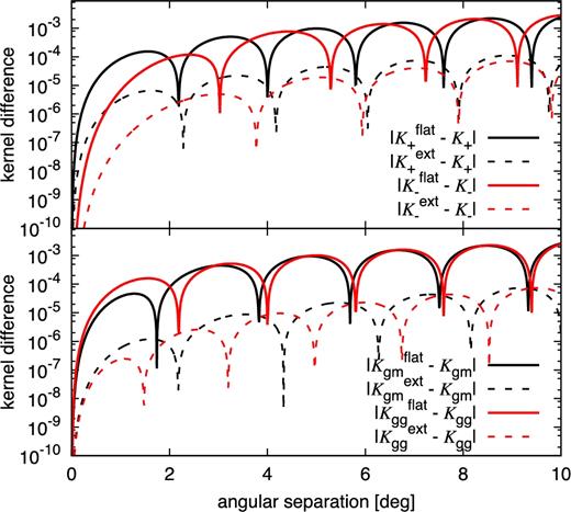
Comparison between kernels in the conversion from correlation functions to power spectra. Shown is the difference between the standard flat-sky (|${\cal K}^{\rm flat}$|, solid lines), as well as the extended flat-sky (|${\cal K}^{\rm ext}$|, dashed lines), approximation and the exact full-sky kernel as a function of angular separation for fixed ℓ = 100. The top panel shows the cosmic shear kernels relating to ξ±; the bottom panel those for Pgm and Pgg.
We compare the power spectrum estimates under the assumptions of the standard and extended flat-sky approximations in the case of galaxy clustering, which extends to the largest angular scales and should thus be most affected. As expected, we find the largest discrepancy for the lowest ℓ bin, which amounts to a relative difference of 3.3 × 10⁻⁵ in F1 and less than 10−6 in F2. Since the extended flat-sky approximation is typically two orders of magnitude more accurate over the scales used in this analysis (see Fig. F1, bottom panel), this implies that the discrepancy that we have measured is also the one between standard flat-sky approximation and full expression to within |$1\, \, {per \,cent}$|. It is reasonable to expect this discrepancy to be very small because we choose to altogether ignore large scales which are inaccessible from our data, rather than merely misrepresenting their geometry. We have demonstrated in Appendix A that the IBC, resulting from cutting in particular the large scales from the integrals in our estimators, is much larger but still well controlled in our measurements.
APPENDIX G: CROSS-SURVEY COVARIANCE
In this analysis we combine probes from two surveys with substantially different areas, where the smaller survey is fully contained in the larger’s area coverage. While the covariances of individual probes can be modelled analytically with the respective survey footprint over which they are measured, there may be significant cross-variances between probes due to the shared sky that need to be included in the joint likelihood analysis.
