


Abstract
In evolutionary population synthesis (EPS) models, we need to convert stellar evolutionary parameters into spectra via interpolation in a stellar spectral library. For theoretical stellar spectral libraries, the spectrum grid is homogeneous on the effective-temperature and gravity plane for a given metallicity. It is relatively easy to derive stellar spectra. For empirical stellar spectral libraries, stellar parameters are irregularly distributed and the interpolation algorithm is relatively complicated. In those EPS models that use empirical stellar spectral libraries, different algorithms are used and the codes are often not released. Moreover, these algorithms are often complicated. In this work, based on a radial basis function (RBF) network, we present a new spectrum interpolation algorithm and its code. Compared with the other interpolation algorithms that are used in EPS models, it can be easily understood and is highly efficient in terms of computation. The code is written in matlab scripts and can be used on any computer system. Using it, we can obtain the interpolated spectra from a library or a combination of libraries. We apply this algorithm to several stellar spectral libraries (such as MILES, ELODIE-3.1 and STELIB-3.2) and give the integrated spectral energy distributions (ISEDs) of stellar populations (with ages from 1 Myr to 14 Gyr) by combining them with Yunnan-III isochrones. Our results show that the differences caused by the adoption of different EPS model components are less than 0.2 dex. All data about the stellar population ISEDs in this work and the RBF spectrum interpolation code can be obtained by request from the first author or downloaded from http://www1.ynao.ac.cn/∼zhangfh.
1 INTRODUCTION
The method of evolutionary population synthesis (EPS) plays an important role in many fields of astronomy. It can be used to derive the stellar mass, metallicity and photometric redshift of galaxies. Combined with photoionization models it can be used to derive the calibrations of the star-formation rate in terms of the luminosities of the H α recombination line and the [O iii] λ 3727 Å forbidden line, and the selection criterion between star-forming galaxies and active galactic nuclei. Finally, combined with galaxy models, it can be used to present the statistical properties of galaxies at different redshifts.
EPS models were first introduced by Tinsley (1968) and consist of the following three key ingredients: (i) a stellar evolution library, used to calculate isochrones in the colour–magnitude diagram; (ii) a stellar spectral library, used to derive the integrated spectral energy distribution (ISED), magnitudes and colours; and (iii) the initial mass function (IMF), used to evaluate the relative proportions of stars in the various evolutionary phases.
EPS models have made great progress, but uncertainties still exist in their two principal building blocks: stellar evolution models (such as the evolution of low-mass stars, the evolution of massive stars and binary stars, and so on) and spectral libraries. Therefore, in recent decades, EPS models have focused on the improvement of these two ingredients. (1) In EPS models using improved stellar evolution models, Maraston (2005, hereafter M05) and Bruzual (2007) have included the thermally pulsing asymptotic giant branch evolution of low- and intermediate-mass stars; Thomas, Maraston & Bender (2003) have used enhanced α-element stellar evolutionary models; Zhang et al. (2004) have considered binary evolution; and Levesque et al. (2012) and Leitherer et al. (2014) have included stellar rotation. (2) In EPS models using improved stellar spectral libraries, the empirical and high-resolution libraries are especially focused on: Bruzual & Charlot (2003, hereafter BC03) have used the empirical STELIB (Le Borgne et al. 2003) and Pickles (1998) libraries; Vazdekis et al. (2010, hereafter V10) have used the empirical MILES library (Cenarro et al. 2007); and Le Borgne et al. (2004) have used the high-resolution ELODIE library (Prugniel & Soubiran 2001) in their PEGASE-HR EPS models.
In general, theoretical stellar spectral libraries have regularly distributed model grids, relatively large coverage of stellar parameters and are at high resolution. The interpolation calculation in them is relatively easy. Then, why do we prefer to use empirical stellar spectral libraries? This is because the abundance pattern for elements in stellar atmospheres is uncertain, the atomic and molecular line lists are incomplete, and so on (Kurucz 2014). The spectra in empirical stellar spectral libraries are obtained from observations and are unlimited by theoretical calculations. The reason that we choose to use high-resolution stellar spectra is that they can provide more and better information and increase our ability to disentangle the age and metallicity degeneracy of stellar populations (SPs) (Worthey 1994).
Although we prefer the empirical spectral libraries in our calculation, this doesn't mean that it do not have limitations. The stars of the empirical stellar spectral library are usually close to the Sun and their metallicities are similar to solar values, few massive stars are included, and the coverage of stellar-atmosphere parameters and wavelength range is relative small. The interpolation is also relatively complicated.
In fact, the spectrum interpolation algorithm is not only used in the EPS models, but also in the stellar spectral fitting codes. Wu et al. (2011) and Prugniel, Vauglin & Koleva (2011) have even used a polynomial-like interpolation algorithm in their stellar spectral fitting codes, which are used to derive the set of stellar-atmosphere parameters. Moreover, in EPS models, the starburst99 code has assigned a star with the spectrum of the nearest point on the |$T\rm _{eff}$|–|$\lg g$| plane; the models in V10 used a relatively complicated Gaussian-like interpolation algorithm, which is described in appendix B of Vazdekis et al. (2003, hereafter V03 algorithm). Except for starburst99, the spectrum interpolation codes have not been released for these spectral fitting codes and EPS models. Therefore, we must build a code when using an empirical spectral library. If a common interpolation code does not exist, one of the disadvantages is that, when several EPS models use different interpolation algorithms, it is difficult to distinguish between the discrepancies in the results introduced by stellar evolution models and those introduced by the spectral library.
In this work, we present a new spectrum interpolation algorithm, which is based on the radial basis function (RBF) network. Compared with the other interpolation algorithms used in the stellar spectral library, it is computationally efficient and can be easily understood and changed. It is written in matlab scripts and can be used on any computer system. Using this code, we can obtain the interpolated spectra from any empirical library or a combination of several libraries. Moreover, in this work, we first apply this algorithm to the MILES empirical stellar spectral library (Sánchez-Blázquez et al. 2006) and present the SP ISEDs from 1 Myr to 14 Gyr by combining them with the Yunnan-III isochrones (Zhang et al. 2013). We use the semi-empirical BaSeL-3.1 stellar spectral library (Lejeune, Cuisinier & Buser 1997; Lejeune, Cuisinier & Buser 1998; Westera et al. 2002) to compare them with the results of V10, BC03 and M05 and analyse the effects of the EPS model ingredients on the results. Finally, we apply this algorithm to the STELIB-3.2 (Le Borgne et al. 2003) and ELODIE-3.1 (Prugniel et al. 2007) spectral libraries.
The outline of the paper is as follows. In Section 2 we describe the RBF interpolation algorithm, its application to the MILES empirical spectral library, the comparison between the derived and original spectra, and the usage of this code. In Section 3, we describe the components in our EPS models and the calculation method of SP ISEDs. In Section 4, we present the ISED effect analysis of EPS model ingredients and the interpolation algorithm on the SP ISED. In Section 5 we show that the RBF algorithm can be easily used in other stellar empirical libraries, and give the corresponding SP spectra. Finally, in Section 6, we give a summary and conclusions.
2 THE RBF INTERPOLATION ALGORITHM AND ITS APPLICATION TO THE STELLAR SPECTRAL LIBRARY
Here, we will describe the RBF interpolation algorithm in Section 2.1 (one-dimensional data in Section 2.1.1 as an example and three-dimensional data corresponding to the stellar spectral library in Section 2.1.2), its application to the MILES spectral library in Section 2.2, and the usage of our released code in Section 2.3.
2.1 RBF interpolation algorithm
The RBF interpolation is realized by a linear combination of radial basic functions (RBFs) and can be used to obtain the output data of any point in the input data space. It was introduced many years ago, and is widely used in many fields (such as mineral analysis, aircraft design, image processing and so on).
The first step in RBF interpolation is to choose the RBF type, then obtain these RBFs’ coefficients by fitting the points in the sample. The RBFs and the corresponding coefficients constitute the necessary interpolated fitting function, by which we can interpolate the output for any input data.
For interpolation in an empirical spectral library, xi, xj and xf in equations (2) and (3) should be three-dimensional values (stellar parameters); yf corresponds to the interpolated flux arrays (flux in the unit interval at different wavelengths) and yj corresponds to the flux array of the jth sample star. In order to better understand the RBF interpolation used in this work, we first use it with one-dimensional sample data in Section 2.1.1.
2.1.1 A simple example of RBF interpolation
We first use the one-dimensional sine function y = 2sin (x) (0 ≤ x ≤ π) to generate 11 points (xi, yi, i = 1, …, 11) as the sample library used in this part. We then use the combination of 11 Gaussian functions to fit the 11 points in the sample library (as shown in equation 3) and obtain the coefficients and the fitting function (see equation 2). Finally we can use the derived fitting functions to get the y value for any x.
In Fig. 1, we illustrate this process. In the top panel, the dashed line represents the function y = 2sin (x); solid lines are for the Gaussian basic functions. In both panels, solid circles are the sample points that are selected from function y = 2sin (x) (xi, yi). In the bottom panel, dashed lines represent the product of fitting the coefficients and the corresponding Gaussian functions; the solid line represents the derived fitting function. By comparison, we see that the fitting function matches well the function y = 2sin (x) in the x range [0, π].
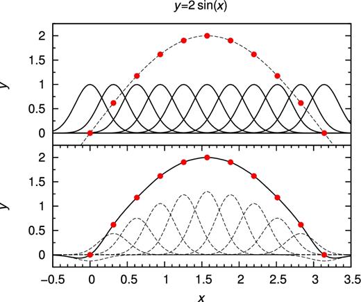
Illustration of a simple example of RBF interpolation. In both panels, the red points are the sample points that were picked up from the function y = 2sin (x). In the top panel, the dotted line is the function y = 2sin (x) and the solid lines represent a set of Gaussian RBFs. In the bottom panel, the dotted lines are the product of the coefficient and corresponding Gaussian RBF and the solid line represents the fitting curve.
2.1.2 RBF interpolation in the empirical stellar spectral library
Repeating the above calculation nl times, we can obtain the interpolated spectrum |$Y^{\prime }_{l,f}$|.
In our work, the above process is realized by matlab scripts and also octave scripts, which can be run on Linux, Windows and MacOS systems.
2.2 Application to the MILES stellar spectral library
In this part, we will apply the code to the MILES stellar spectral library (a description of which will be given in the next section) and give the comparison between the interpolated and original spectra as the first and direct test.
2.2.1 Other treatments
Before the RBF interpolation calculations, we first do the following two pretreatments.
We obtain the conversion factors h1, h2 and h3 in equation (4). Letting the distribution ranges of X1 i, X2 i and X3 i be 7, we obtain h1 = 3.9, h2 = 1 and h3 = 1.4.
- We need to get the normalized spectra in the library. This step is to ensure that the input spectra has a fixed format no matter what kind of flux (normalized, absolute, surface, etc.) is provided by the spectral library and what kind of library (empirical, theoretical) it is. First, we get the integrated V-band flux (Johnson–Cousins system), (FVori)j, based on the following integral:where (Yori)l j is the unit interval flux at the lth wavelength of the jth star in the library, Pl is the transmission curve of the V-band filter at the lth wavelength, and dλl is the wavelength interval between the l and the (l − 1) wavelengths. Then, we can get the normalized flux:(8)\begin{equation} (F_{V{\rm ori}})_j = \sum _{l = 1}^{n_l}(Y_{\rm ori})_{l\,j}\times P_{l}\times \rm d\lambda _l, \end{equation}Yl j is the flux used in equation (6). Solving the linear equations of equation (6), we can get the coefficient matrix Cl i.(9)\begin{equation} {Y_{l\,j}} = (Y_{\rm ori})_{l\,j}/(F_{V{\rm ori}})_j, \end{equation}
Furthermore, we can get the interpolated flux |$Y^{\prime }_{l,f}$|, but it is dimensionless divided by Å. We need two steps to convert it to the unit area flux on the stellar surface.
- The first step is to renormalize the interpolated flux |$Y^{\prime }_{l,f}$| by its V-band flux |$(F_V^{\prime })_f$|. Adopting the same method as in equations 8 and 9, we can get |$(F_V^{\prime })_f$|:where |$Y^{\prime }_{l,f}$| is given by equation (5). Then, we can get the flux normalized to the V-band flux |$f_{l,f}^{\prime }$|:(10)\begin{equation} (F_V^{\prime })_f = \sum _{l = 1}^{n_l}Y_{l,f}^{\prime }\times P_{l}\times \rm d\lambda _l, \end{equation}(11)\begin{equation} f_{l,f}^{\prime } = Y_{l,f}^{\prime }/(F_V^{\prime })_f . \end{equation}
- The second step is to transform the normalized flux |$f_{l,f}^{\prime }$| to the stellar surface flux fl, f. The flux of equation (11) is in units of Å−1. In order to use |$f_{l,f}^{\prime }$| in the EPS models, we need to transform it to the unit area flux on the stellar surface fl, f (in units of |$\rm erg\,s^{-1}\,$|Å|$^{-1}\,\rm cm^{-2}$|). The method is as follows:where |$f^{\prime }_{l,f}$| is the normalized flux (equation 11), (FVtho)f is the unit area V-band flux on the stellar surface (in units of erg s−1 cm−2) for Xp, f. (FVtho)f is actually obtained by taking advantage of the BaSeL-3.1 library and linear interpolation algorithm, because the BaSeL-3.1 stellar spectral library also uses the Johnson–Cousins system. We obtain the bolometric correction (B.C.) for Xp, f, then use |$(F_{V{\rm tho}})_f = 10^{[(\mathrm{B.C.})_f+2.5\lg (\sigma T^4_{\mathrm{eff},f})+ D]/2.5}$| (σ is the Stefan–Boltzmann constant, D is a constant regarding the zero magnitude and Teff, f corresponds to X1, f, as shown in equation 4) to get it.(12)\begin{equation} f_{l,f} = f^{\prime }_{l,f} \times (F_{V{\rm tho}})_f, \end{equation}
After the calculations from Sections 2.1 to 2.2.1, which is the standard process for our RBF interpolation algorithm in a stellar spectra library, we can obtain the interpolated spectra on the stellar surface.
2.2.2 Comparison of the interpolated spectra with those in the library
In this part, we perform the test by using the stars in the library. The method and process are as follows.
First, we choose any star (A) from the MILES library as the test point, and move it out from the MILES library.
Secondly, we put the new library (without the test point) into the standard process to get the interpolated spectrum by using the parameters of the A-star. The new coefficient matrix |$C_{l\,i}^{\prime }$| is different from Cl i in equation (7). This is because only N − 1 points will be used in the above set of calculations, the standard deviation (|$\sigma _i^{\prime }$|) of the ith star around point A changes according to the definition below equation (5), and the number of equations and the number of RBFs in equation (6) decreases.
In Fig. 2, we show the comparisons in the spectra for six test stars from the MILES library. These six test stars are randomly selected. In the upper part of each panel, the black line is the original spectrum (Yori)l j (see equation 9), and the red line is the modified RBF interpolated spectrum |$Y^{\prime \prime }_{l,f}$| [|$\equiv \frac{ Y^{\prime }_{l,f} \, \sum _{l = 1}^{n_l} (P_{l} \, \rm d\lambda _l) }{ \sum _{l = 1}^{n_l} (Y^{\prime }_{l,f} \, P_{l} \, \rm d\lambda _l) }$|; refer to equation 10 for |$Y^{\prime }_{l,f}$|. The reason for using |$Y^{\prime \prime }_{l,f}$| is that our spectrum normalization method is different from that used in the MILES library]. In the lower part of each panel, we also present the corresponding flux difference Δ [|$\equiv (Y_{\rm ori})_{l\,j}-Y^{\prime \prime }_{l,f}$|]. From these, we see that they agree well with each other.
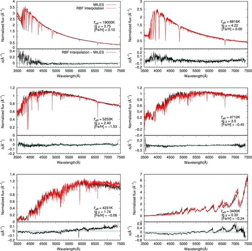
Comparison of the normalized spectra for six different stars, for which the effective temperature, gravity and metallicity are given in the bottom right-hand corner of the upper part of each panel. In each of these parts, the original MILES spectrum ((Yori)l j; see equation 8) and the modified RBF interpolated spectrum (|$Y^{\prime \prime }_{l,f}$|; see text) are represented by black and red lines, respectively. In the lower part of each panel, the corresponding flux difference Δ is given (see text for details).
2.3 Usage
In this section, we will simply describe how to use our RBF interpolation code. First you must confirm that in the spectral library all stars have different input parameters (if different spectra have the same stellar parameters, equation 6 will be singular). Secondly, ensure that all data in the library are in the required format (the format requirements are given by the readme file, available as described in the abstract).
The code includes the stellar-parameter transformation (equation 4), spectrum normalization (equation 9), the coefficient matrix Cl, i calculation (equation 6), and the interpolated result |$Y^{\prime }_{l,f}$| calculation (equation 5). Finally, equations (11) and (12) convert |$Y^{\prime }_{l,f}$| to output spectra of the unit area on the stellar surface.
3 MODEL DESCRIPTION
In our EPS models, the calculation process of the SP ISED is as follows. First, we obtain the evolutionary parameters of stars (with minit, Z and age t) in the given SP from the isochrone data. Secondly, we transform the stellar evolution parameters to the stellar spectrum. Thirdly, we use the IMF to get the number proportions of stars in the initial-mass range m → m + dm (in our calculations, the SP mass is normalized to 1 |$\rm M_{\odot }$|). Finally, we derive the ISEDs of SPs by integrating the product of the spectrum and the number proportion over the initial-mass range.
In Section 3.1, we briefly describe the constituents used in these EPS models. In Section 3.2, we give the calculation process of the SP ISEDs.
3.1 The components of our EPS models
In this work we use the isochrones from the Yunnan-III EPS models and those of Girardi et al. (2000, hereafter G00), MILES (Sánchez-Blázquez et al. 2006), ELODIE-3.1 (Prugniel et al. 2007), STELIB-3.2 (Le Borgne et al. 2003) empirical and BaSeL-3.1 (Lejeune et al. 1997; Lejeune et al. 1998; Westera et al. 2002) semi-empirical stellar spectral libraries, and the Salpeter (1955, hereafter S55) and Kroupa (2001, hereafter K01) IMFs.
The isochrones in the Yunnan-III EPS models (Zhang et al. 2013) were calculated based on the mesa stellar evolution code (Paxton et al. 2011). The SPs are at solar metallicity and their ages range from |$\lg (t\,\mathrm{yr}^{-1}) = 6.0$|–10.15 at an interval of 0.05 dex. The G00 isochrones are based on the evolutionary tracks of low- and intermediate-mass stars (from 0.15 M⊙ to 7 M⊙) and were built by the Padova group. The metallicity of the G00 isochrones is from Z = 0.0004–0.03 (we only use the results at Z = 0.02) and the age is from |$\lg (t\,\mathrm{yr}^{-1}) = 7.8$|–10.25 at an interval of 0.05 dex.
In this section, we only describe the MILES and BaSeL-3.1 spectral libraries; the STELIB-3.2 and ELODIE-3.1 libraries will be described in Section 5. (i) The MILES empirical stellar spectral library includes the spectra of 985 stars that were obtained on the 2.5 m Isaac Newton Telescope. The wavelength ranges from 3540.5 Å to 7409.6 Å and the spectral resolution is ∼2.3 Å (FWHM, Sánchez-Blázquez et al. 2006). The coverages of the stellar-atmosphere parameters are: 2748 K < Teff < 36 000 K, |$0.00< \lg g<5.50$| and −2.93 < [Fe/H] < +1.65. The MILES spectral library has a larger coverage in the parameter spaces than the other empirical stellar spectral libraries that are used in the EPS models (Cenarro et al. 2007). (ii) The BaSeL-3.1 semi-empirical stellar spectral library is based on theoretical spectral libraries (from O to late-K stars, M-giants and M-dwarfs, respectively). It provides an extensive and homogeneous grid of low-resolution spectra in the range of 91–1600 000 Å for a large range of stellar parameters: 2000 K < Teff < 50 000 K; |$-1.02< \lg g< 5.5$| and −5.0 < [Fe/H] < 1.0. When using the BaSeL-3.1 spectral library in the EPS models or stellar spectral fitting code, linear interpolation is often used. Moreover, the BaSeL-3.1 library provides the unit area flux on the stellar surface, so it is different from the empirical library.
Finally, we use the S55 IMF with a slope of −2.35 and K01 IMF. The lower and upper mass limits (ml, mu) are 0.1 and 100|$\,\rm M_{\odot }$|, respectively.
3.2 Algorithm of the SP ISED
4 RESULTS, ANALYSIS AND DISCUSSIONS
In this work, we build five sets of models. Each model differs from the others mainly by changing one of the EPS model ingredients. The characteristics of each model are summarized in Table 1, where columns 2 to 4 give the details of the EPS ingredients (isochrone, stellar spectral library and IMF) and spectrum interpolation algorithm (column 3), and columns 5 to 6 describe the ISED wavelength, age range and age interval of the SSPs .
Characteristics of Models A–F. Columns 2–4 give the details of the EPS ingredients (isochrone, stellar spectral library and IMF) and spectrum interpolation algorithm (column 3). Columns 5–6 are the descriptions of the ISED wavelength range, age range and age interval of single stellar populations (SSPs).
| Model | Isochrone | Stellar spectral library & | IMF | Wavelength range (Å) | Age range and interval (|$\lg (t\,\mathrm{yr}^{-1})$|) |
|---|---|---|---|---|---|
| interpolation algorithm | |||||
| A | Yunnan-III | MILES & RBF | S55, K01 | 3540.5–7409.6 | 6.0–10.15, 0.05 |
| B | Yunnan-III | BaSeL-3.1 & Linear | S55 | 90.0–1600 000.0 | 6.0–10.15, 0.05 |
| C | G00 (Z ≥ 10−4) | MILES & RBF | S55 | 3540.5–7409.6 | 7.8–10.25, 0.05 |
| D | Yunnan-III | MILES(BaSeL) & RBF | S55 | 3540.5–7409.6 | 6.0–10.15, 0.05 |
| E | Yunnan-III | STELIB(BaSeL) & RBF | S55 | 3200.0–9500.0 | 6.0–10.15, 0.05 |
| F | Yunnan-III | ELODIE-3.1 & RBF | S55 | 3900.0–6800.0 | 6.0–10.15, 0.05 |
Model A adopts the isochrones from the Yunnan-III EPS models, the MILES stellar spectral library and the S55 and K01 IMFs (hereafter A-S55 and A-K01). Our standard is Model A. In the following, the S55 IMF has a slope of −2.35. Model B differs from A by adopting the semi-empirical BaSeL-3.1 stellar spectral library and the corresponding linear spectrum interpolation algorithm. For Model B, a linear spectrum interpolation algorithm is used because the spectrum grid of the BaSeL-3.1 spectral library is homogeneous. Model C differs from A by using the G00 isochrones. Models D–F differ from Model A by adopting a different stellar spectral library. In Models D and E, we do not use the original spectra provided by the MILES and STELIB libraries, but use a set of artificial spectra, which are obtained by using the stellar parameters of the corresponding library and the linear interpolation algorithm of the BaSeL-3.1 spectral library. In Model F, we use the ELODIE-3.1 library directly. For Models B–F, we only present the results with the S55 IMF.
Models B–D are mainly used to investigate the effects of the stellar spectral library, spectrum interpolation algorithm and isochrone (Sections 4.1.2 and 4.1.3) on the SSPs ISED. The reason for using G00 isochrones in Model C is that the V10 model with the S55 IMF has the same EPS model ingredients except for the stellar spectrum interpolation algorithm. Taking advantage of them, we can analyse the effect of the spectrum interpolation algorithm on the SP ISEDs. Model D is used to analyse the difference in the SP colour between Models A and B. Models E and F are used to show that this algorithm is universal to the other empirical stellar spectral libraries (Section 5).
In this work, the age of the SSPs ranges from 106.0 to 1010.15 yr for all models except for Model C (from 107.8 to 1010.25 yr at a logarithmic age interval of 0.05 dex). The wavelength of ISEDs ranges from 3540.5 to 7409.6 Å with a resolution of ∼2.3 Å for Models A and C (MILES library) and a resolution of ∼20 Å for Model D (MILES+BaSeL-3.1 libraries), 90 to 1600 000 Å with a resolution of ∼20 Å for Model B (BaSeL-3.1 library), 3200.0 to 9500.0 Å with a resolution of ∼20 Å for Model E (STELIB+BaSeL-3.1 libraries), and 3900.0 to 6800.0 Å with a resolution of R = 10 000 for Model F (ELODIE-3.1 library).
In Section 4.1 we will present the results of Models A–D, compare the results of Model A with B and those of Model C with the V10 models, analyse the effects of the IMF, stellar spectral library, spectrum interpolation algorithm (by comparison with the V10 models) and isochrone on the SP ISEDs, and give comparisons between our results and the BC03 and M05 models in Section 4.2. All results in this part are at solar metallicity. In order to test the ability of our RBF algorithm at low metallicity or in sparse regions of atmosphere parameters, in Appendix A, we also present the SP ISEDs of Model C at [Fe/H] = −0.4, −0.7, −1.3 and −1.7, and compare them with the V10 models.
4.1 Results of Models A–C and effects of EPS model ingredients
In Section 4.1.1, we will first present the results of Model A and analyse the effect of IMF on the SP ISED, in Section 4.1.2 we give the results of Model B and show the differences in the ISEDs caused by the usage of the MILES and BaSeL-3.1 stellar spectral libraries, in Section 4.1.3 we give the results of Model C and analyse the effects of isochrone (between Yunnan-III and G00) and spectrum interpolation algorithm (between the V03 algorithm and RBF) by comparing Model A with C and Model C with V10, respectively, and summarize the differences caused by the above factors in the SP ISED in Section 4.1.4.
4.1.1 Results of Model A and the effect of IMF
We explore the ISED evolution of Model A and find that the flux first increases (|$t \lesssim 10^{6.45}$| yr) and then decreases with increasing age for both the A-S55 and A-K01 models. In Fig. 3 we give the SP ISEDs of Model A; for the sake of clarity, only the results with ages in the range |$6.0 \leqslant \lg (t\,\mathrm{yr}^{-1}) \leqslant 9.9$| at a logarithmic age interval of 0.3 dex and |$\lg (t\,\mathrm{yr}^{-1}) = 10.15$| are shown. When the SP age is greater than |$\lg (t\,\mathrm{yr}^{-1}) = 6.9$|, the results of Models A-S55 and A-K01 are represented by black and red lines, respectively; when |$\lg (t\,\mathrm{yr}^{-1}) = 6.0$|, 6.3 and 6.6 they are represented by grey, blue and green lines (from bottom to top; at a given age, the higher flux is the result of K01). From Fig. 3, we see that the evolution of SSPs ISEDs has a turn-off as mentioned above; the reason for this is that massive stars begin to leave the main sequence.
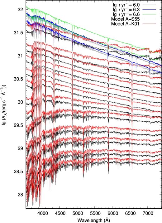
The SP ISEDs for Models A-S55 and A-K01. For the sake of clarity, only the results with ages in the range |$6.0 \le \lg (t\,\mathrm{yr}^{-1}) \le 9.9$| at a logarithmic age interval of 0.3 dex and |$\lg (t\,\mathrm{yr}^{-1}) = 10.15$| are plotted. Black and red lines are for the S55 and K01 IMFs, respectively, when age is greater than 106.6 yr. Grey, blue and green lines are the results for SPs at ages of 106.0, 106.3 and 106.6 yr (from bottom to top).
Moreover, from Fig. 3 we see that the A-K01 models have larger fluxes than the A-S55 models (insignificant for old SSPs at the blue end of the optical region) for SPs at all ages. The reason for this is that the number of stars with |$M\gtrsim 0.4$| M⊙ for the K01 IMF is greater than that of the S55 IMF. Those stars with |$M\gtrsim 0.4$| M⊙ are the main contributors of optical flux for both young and old SPs.
4.1.2 Results of Model B and the effect of the stellar spectral library
Model B uses the semi-empirical BaSeL-3.1 spectral library and the ISEDs cover a wider wavelength range (90 Å–1600 000 Å). Moreover, only the results with the S55 IMF are given.
First, we explore the evolution of the SSPs ISEDs of Model B and find that it is similar to Model A, i.e. the flux increases when the age decreases (with a turn-off at t ∼ 106.45 yr). When comparing the ISEDs of Model B with A-S55, we find that the ISEDs agree well in the wavelength range 3540.5 ≤ λ ≤ 7409.6 Å for SPs with ages in the range of |$\lg (t\,\mathrm{yr}^{-1}) = 6.8$|–10.15, but there is a larger discrepancy in the range of |$6.0\le \lg (t\,\mathrm{yr}^{-1})\le 6.8$|. When |$\lg (t\,\mathrm{yr}^{-1})<6.8$|, Model B has a higher flux and a similar slope; at |$\lg (t\,\mathrm{yr}^{-1}) \sim 6.8$|, the flux of Model B is far higher than that of Model A at the red end. The differences may be caused by the following factors. In young SPs, the temperature of some stars along the isochrone is very high; in Model B we use the blackbody spectrum when Teff is beyond the coverage of the BaSeL-3.1 spectral library. In Model A-S55 we still use the RBF interpolation algorithm although hot stars are rare in the MILES library.
In Fig. 4, we give the comparison in the ISED evolution between Models A-S55 and B. For the sake of clarity, only the results in the common (visible) passband for SPs with ages in the range |$7.0\le \lg (t\,\mathrm{yr}^{-1})\le 10.0$| at a logarithmic age interval of 0.3 dex are given. From it, we see that the results agree with each other for Models A and B; the maximum continuum difference is ∼0.02 dex. The ISEDs of Model A-S55 are greater at the blue end of the optical range (|$\lambda \lesssim 4500$| Å) when |$7.0 \lesssim \lg (t\,\mathrm{yr}^{-1}) \lesssim 8.5$| (the first six curves from top to bottom in Fig. 4), and lower at the red end (|$\lambda \gtrsim 5500$| Å) when |$\lg (t\,\mathrm{yr}^{-1})\gtrsim 7.0$| compared to Model B. That is to say, the optical colours of Model A-S55 are bluer than Model B (the absolute value of the ISED slope is larger), and the differences in the colours increase with age when |$\lg (t\,\mathrm{yr}^{-1}) \lesssim 8.2$|.
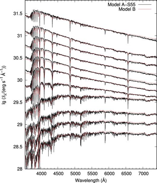
The evolution of SP optical spectra for Models A-S55 (black lines) and B (red lines). The SP ages are in the range of |$7.0 \leqslant \lg (t\,\mathrm{yr}^{-1}) \leqslant 10.0$| (from top to bottom) at a logarithmic interval of 0.3 dex (11 curves).
Which factors lead to the differences in the colours between Models A and B? The differences between Models A and B are the stellar spectral library and the spectrum interpolation algorithm used. The difference in the stellar spectral library lies in their distributions of stellar-atmosphere parameters and their calibration relations. The atmosphere parameters of the MILES spectral library were obtained from different sources (Cenarro et al. 2007), which may cause a self-consistent problem (as noted by Prugniel et al. 2011). In order to discuss the effect of the calibration relations, we build Model D. As described in Table 1, the spectral library of Model D is obtained by using the parameters in the MILES spectral library and the linear interpolation among the BaSeL-3.1 spectral library, and the other ingredients are the same as in Model A-S55. In Fig. 5, we give the results of Models B and D, which are represented by red and black lines, respectively. The SP ages are from |$\lg (t\ \mathrm{yr}^{-1}) = 7.0$|–10.0 at an interval of 0.3 dex (from top to bottom). From Fig. 5, we can see the colour differences existing in Fig. 4 almost disappear at all ages. That is to say, the differences in the colours between Models A and B are mainly caused by the spectrum calibration relations. Moreover, the colour difference introduced by the spectrum calibration relations, i.e. the colour difference between the MILES spectra and the corresponding spectra given by linear interpolation from BaSeL-3.1, is given in Fig. 6. In it, we give the difference in (B − V) colour, Δ(B − V) = (B − V)MILES − (B − V)Model D, between that derived from the spectra of the MILES spectral library and those from the spectral library of Model D. From it, we clearly see that the difference exists.
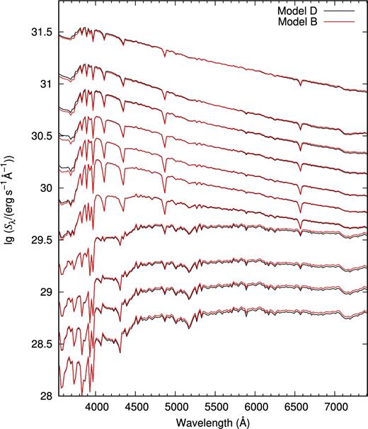
Similar to Fig. 4, but for Models D (black lines) and B (red lines).
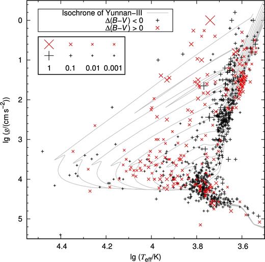
The colour difference Δ(B − V) between (B − V)MILES and (B − V)Model D (see Section 4.1.2 for details). Red ‘×’ and black ‘+’ represent Δ(B − V) > 0 and <0, respectively. Symbol size indicates the absolute value of Δ(B − V). Also shown are Yunnan-III isochrones for SPs with ages in the range of |$\lg (t\,\mathrm{yr}^{-1}) = 7.0$|–10.0 at an interval of 0.3 dex.
4.1.3 Results of Model C, comparison with the V10 model and the effects of the isochrone and spectrum interpolation algorithm
Model C uses the G00 isochrones with ages from |$\lg (t\,\mathrm{yr}^{-1}) = 7.8$|–10.25. In the left-hand panel of Fig. 7, we give the ISEDs of Model A-S55 for SPs with ages in the range of |$\lg (t\,\mathrm{yr}^{-1}) = 7.8$|–9.9 (7.8–10.2 for Model C) at an interval of 0.3 dex. The maximal age of SSPs is |$\lg (t\,\mathrm{yr}^{-1}) = 10.15$| for the Yunnan-III models, |$\lg (t\,\mathrm{yr}^{-1}) = 10.25$| for Model C, so in the left-hand panel of Fig. 7 (also for the isochrone in Fig. 8) the results at |$\lg (t\,\mathrm{yr}^{-1}) = 10.2$| of Model C do not have a counterpart. From the left-hand panel of Fig. 7, we see that Model A-S55 has lower fluxes than Model C but similar colours (similar spectral slope). The differences in the ISEDs can reach ∼0.1 dex at |$\lg (t\,\mathrm{yr}^{-1}) = 7.8$|. The flux difference is mainly caused by the difference in the isochrones.
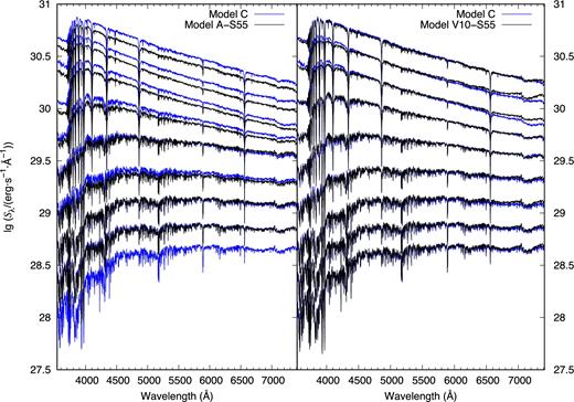
Left: similar to Fig. 4, but for |$\lg (t\,\mathrm{yr}^{-1}) = 7.8$|–10.2 (7.8–9.9 for Model A-S55) and for Models A-S55 (black solid lines) and C (blue solid lines). Right: similar to left-hand panel, but for Models C (blue solid lines) and V10-S55 (black solid lines).

In Fig. 8, we plot the two sets of isochrones that used in Models A and C, the Yunnan-III and G00 isochrones. The G00 isochrones are built based on Padova stellar evolutionary tracks, the Yunnan-III isochrones are based on the mesa stellar evolution model (Zhang et al. 2013). From Fig. 8, we see that the isochrones of the Yunnan-III models lie on the right of the G00 isochrones when |$\lg (t\,\mathrm{yr}^{-1})\leqslant 9.30$|, and the difference decreases with increasing SP age, which is consistent with the variation trend of the ISED difference in the left-hand panel of Fig. 7.
Moreover, we also compare the ISEDs of Model C with the V10 models with the S55 IMF (hereafter V10-S55). Two sets of models use the same ingredients: isochrone, spectral library and IMF. The sole difference is the spectrum interpolation algorithm. These two sets of models can be used to analyse the effect of the spectrum interpolation algorithm on the SP ISED. In the right-hand panel of Fig. 7, we give the ISEDs of Models C and V10-S55. From it, we see that they agree well, and the difference is ∼0.01 dex. Our interpolation algorithm makes the SP ISEDs bluer than those of the V10-S55 model when the SP ages are ∼108.1 yr and 108.4 yr (see the second and third curves from top to bottom in the right-hand panel of Fig. 8).
In fact, for different spectral libraries, the effect is different. For an empirical spectral library (such as MILES), if we use the linear interpolation algorithm, the results are far worse than those calculated by the RBF and V03 interpolation algorithms; the difference in the SP ISED is far larger than 0.01 dex. For a theoretical stellar spectral library (such as BaSeL), the difference made by the adoption of RBF and a linear interpolation algorithm is insignificant in the SP ISED. We have even used the RBF interpolation algorithm in the BaSeL-3.1 library; the results are similar to those given by the linear interpolation. The conclusion of a difference of ∼0.1 dex in the SP ISED, caused by the use of a different spectrum interpolation algorithm, is not true in all cases: it is actually dependent on the choice of spectral library.
4.1.4 Summary of the results
We summarize the maximal differences in the logarithmic flux, |$[\Delta (\lg S_{\lambda })]_\mathrm{max}$|, and the colour, [Δ(B − V)]max, by the adoption of different IMFs, stellar spectral libraries, spectrum interpolation algorithms and isochrones in the third and fourth columns of Table 2. From the third column of Table 2, we see that the maximal flux difference by the adoption of different IMFs (S55 and K01) is ∼ 0.2 dex, that by different stellar spectral libraries (MILES and BaSeL) is ∼ 0.02 dex, that by the adoption of the G00 and Yunnan-III isochrones is ∼ 0.1 dex, and that by different spectrum interpolation algorithms (RBF and V03 interpolation algorithms, in the MILES library) is less than 0.01 dex. The maximal flux differences by the adoption of different IMFs and isochrones are larger than those by different stellar spectral libraries and spectrum interpolation algorithms in this work. From the fourth column of Table 2, we see that the factors of isochrone and interpolation algorithm lead to the largest and smallest [Δ(B − V)]max, respectively. The above difference by spectrum interpolation algorithms is only true for the MILES spectral library; in fact, it is different for different spectral libraries. For example, if the linear interpolation algorithm were to be used in the MILES spectral library, the difference would be very large.
Summary of the discrepancies in the SP results by the adoption of different IMFs, stellar spectral libraries, isochrones and spectrum interpolation algorithms. The third and fourth columns are the maximal differences in the logarithmic flux (|$\lg S_{\rm \lambda }$|) and B − V colour, respectively.
Summary of the discrepancies in the SP results by the adoption of different IMFs, stellar spectral libraries, isochrones and spectrum interpolation algorithms. The third and fourth columns are the maximal differences in the logarithmic flux (|$\lg S_{\rm \lambda }$|) and B − V colour, respectively.
4.2 Comparison with other models
In the above section, we have compared Models A-S55 with the V10-S55 models. In this section, we will compare Models A-S55 with the M05-S55 and BC03-S55 models.
The BC03 models have presented the results by using different stellar evolutionary tracks (Padova-1994, Padova-2000 and Geneva), different stellar spectral libraries (BaSeL, STELIB and Pickles) and the S55 and Chabrier (2003) IMFs. When the BaSeL spectral library is used, the model ISEDs are at low resolution and the wavelength is in the range 91 Å –160 μm . When the STELIB spectral library is used, the ISEDs are at medium resolution (R ≈ 2000) and wavelength is from 3200 to 9500 Å (Bruzual & Charlot 2003). SSPs ages are from 1 × 10⁵ to 2 × 10¹⁰ yr. In this work, we choose the set of solar-metallicity ISEDs with the S55 IMF (hereafter BC03-S55).
The M05 models were built by using the fuel consumption theorem. In their models, a combination of several sets of stellar evolution tracks and isochrones (Cassisi, Castellani & Castellani 1997b; Cassisi, degl'Innocenti & Salaris 1997a; Cassisi et al. 2000, Geneva and Padova group), the BaSeL-3.1 stellar spectral library and the S55 and K01 IMFs were used. In this work, we use the set of solar-metallicity ISEDs, which were obtained by using the red horizontal branch (RHB) evolutionary results (Maraston 2005) and the S55 IMF (hereafter M05-S55).
In the left-hand panel of Fig. 9, we give the comparison of the ISEDs between the BC03-S55 and A-S55 models, and that between the M05-S55 and A-S55 models in the right-hand panel. The younger SPs have significantly different ISEDs. We only present the flux within 3540.5–7409.6 Å for SPs with ages from |$\lg (t\,\mathrm{yr}^{-1}) = 7.0$|–10.0 at an interval 0.3 dex and |$\lg (t\,\mathrm{yr}^{-1}) = 10.15$|.

From the left-hand panel of Fig. 9, we see that the ISEDs show a large discrepancy when |$\lg (t\,\mathrm{yr}^{-1})<8.8$|. The flux of Model A-S55 is lower than BC03-S55, but the colour (ISED slope) is similar when |$\lg (t\,\mathrm{yr}^{-1})\geqslant 7.6$|. The difference decreases with increasing age.
From the right-hand panel of Fig. 9, we see that Model A-S55 has a lower flux and bluer colours than the M05-S55 models. The flux difference increases when the wavelength increases.
5 SP ISEDS BY USING OTHER STELLAR SPECTRA LIBRARIES
The above results reveal that our RBF spectrum interpolation code can easily be used in the MILES library. Can it be conveniently used in the other empirical stellar libraries? In this section, we will use the STELIB-3.2 and ELODIE-3.1 empirical stellar spectral libraries in the Yunnan-III EPS models to show the ability of our RBF spectrum interpolation code.
5.1 Application to the STELIB-3.2 and ELODIE-3.1 libraries
The STELIB library consists of 249 stellar spectra obtained on the 1 m Jacobus Kapteyn Telescope (JKT) and the 2.3 m telescope of the Australian National University at Siding Spring Observatory (SSO) (Le Borgne et al. 2003). The wavelength range is from 3200 to 9500 Å and the spectral resolution is less than 3 Å. The ranges of stellar parameters: |$3162\,\mathrm{K}<T_{\rm eff}<39\,810\,\mathrm{K}, 0<\lg g<5$| and −3 < [Fe/H] < 0.8 (shown in Figs 3 and 4 of Bertone et al. 2008). In this study, we use the 3.2 version of STELIB library.
The spectra in the ELODIE-3.1 library were observed with the ELODIE spectrograph on the Observatory de Haute Provence 193 cm telescope. The spectral wavelength range is 3900 to 6800 Å, the high (R = 42 000) and the intermediate (R = 10 000) resolutions are provided. The ranges of the stellar parameters are 3100 K <Teff < 50 000 K, |$-0.25<\lg g<4.9$| and −3 < [Fe/H] < 1.0 (Prugniel et al. 2007). In this work, we use the 3.1 version and the R = 10 000 library, which includes 1962 spectra of 1388 stars.
Before the RBF spectrum interpolation calculations, we need to do some pretreatments for these two spectral libraries. (1) In the MILES library, all spectra have the same wavelength range, while in the STELIB library, many spectra have a shorter wavelength range than the standard one (3200–9500 Å). For simplicity, we use artificial spectra to replace the original ones. The method is same as in Model D (i.e. we use the stellar parameters provided by the STELIB-3.2 library and the linear interpolation algorithm in the BaSeL-3.1 spectral library to produce those spectra in 3200–9500 Å). (2) In the ELODIE-3.1 spectral library, there exist two special cases. One is that a star (a set of coordinates) has several sets of stellar parameters and spectra, another is that a star has a set of stellar parameters and several sets of spectra. In the first case, we treat it as several stars, in the second case, we use its average spectrum. Finally, we get 1458 spectra.
Inputting these two empirical libraries into our standard RBF interpolation code, which is described in Sections 2.1 to 2.2.1, we can obtain the interpolated spectra on the stellar surface.
5.2 Results of SPs
Combining the S55 IMF and Yunnan-III isochrones, we obtain the SP ISEDs. These two sets of models are called Models E and F, respectively (Table 1).
The results are plotted in Fig. 10. The left-hand panel gives the comparison in the SP ISED between Models A-S55 (black lines) and E (grey lines), the right-hand panel is that between Models A-S55 (black lines) and F (red lines). For the sake of clarity, in Fig. 10, only the results with ages in the range of |$\lg (t\,\mathrm{yr}^{-1}) = 7.0$|–10.0 at an interval of 0.3 dex and |$\lg (t\,\mathrm{yr}^{-1}) = 10.15$| (the bottom line) are shown. From the left-hand panel of Fig. 10, we see that Models A-S55 and E agree well. From the right-hand panel, we see that the colours are significantly different from that of Model A-S55 when age |$\lg (t\,\mathrm{yr}^{-1}) \lesssim 8.5$| (many factors could cause this difference, such as our pretreatments for ELODIE's spectral data, described in Section 5.1, or the incomplete cover of the stellar-parameter distributions). Moreover, the differences in the SP ISEDs between Models A-S55 and F are similar to those between A-S55 and B in Section 4.1.2.
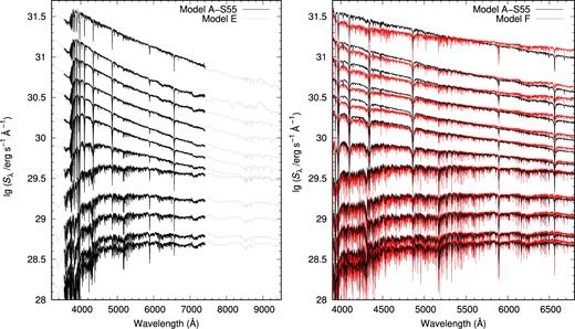
Finally, the comparisons shown in Fig. 10 can confirm that our RBF interpolation code can be conveniently applied to different stellar spectral libraries.
6 SUMMARY AND CONCLUSIONS
In this work, we first build a stellar spectrum interpolation algorithm based on the RBF network, then use it in the empirical MILES spectral library. Combined with the isochrones of the Yunnan-III EPS models and the S55 and K01 IMFs, we obtain SP ISEDs. The SP ages are from 106–1010.15 yr, the wavelength range is from 3540.5–7409.6 Å and the spectral resolution is ∼2.3 Å. Our results show that the SP ISEDs agree well with those obtained by using the semi-empirical BaSeL-3.1 spectral library and the linear interpolation algorithm and those of V10, BC03 and M05 EPS models.
By comparing with the results obtained by using different EPS components and the results of other EPS models, we find that the maximal discrepancy in the SPs’ logarithmic flux, |$[\Delta (\lg S_{\lambda })]_{\rm max}$|, by the adoption of different IMFs (S55 and K01) is less than ∼ 0.2 dex, the difference by different isochrones (G00 and Yunnan-III) is less than ∼ 0.1 dex, that by different stellar spectral libraries (MILES and BaSeL, RBF interpolation algorithm) is less than ∼ 0.02 dex, and that by different spectrum interpolation algorithms (ours and the V03 algorithms, in the MILES library) is less than ∼0.01 dex. The maximal colour differences, [Δ(B − V)]max, are less than ∼0.07, ∼0.09, ∼0.08 and ∼0.04 mag, respectively. The differences by the adoption of different IMFs and isochrones are larger than those by different stellar spectral libraries and spectrum interpolation algorithms. If the linear interpolation algorithm were to be used, the difference caused by the stellar spectral libraries (MILES and BaSeL) would be very large.
Moreover, we also use the RBF interpolation algorithm in the empirical spectral STELIB-3.2 and ELODIE-3.1 libraries. Results show that this algorithm not only has a rapid calculation speed but also can be easily used in the other empirical libraries. Meanwhile, its mathematical description is easily understood and is easy to change according to need. For example, you can replace the Euclidean distance in equations (4)–(6) with a new metric tensor to define the distance in stellar-parameter space as the interpolation scale. All data on Models A–F and the code of the RBF algorithm can be obtained from the first author or requested from http://www1.ynao.ac.cn/∼zhangfh.
ACKNOWLEDGEMENTS
This project was partly supported by the Chinese Natural Science Foundation (No. 11573062, 11373063, 11273053, 11390374, 1152100017 and 11403092), the YIPACAS Foundation (No. 2012048), and the Yunnan Foundation (grant No. 2011CI053). We also thank the referee for suggestions that have improved the quality of this manuscript.
REFERENCES
APPENDIX A: RESULTS AT LOW METALLICITY
In this appendix, we will give the SP ISEDs for Model C at low metallicity ([Fe/H] = −0.4, −0.7, −1.3 and−1.7), and compare them with the V10-S55 models. Model C uses the same EPS ingredients as the V10-S55 models except for the spectrum interpolation algorithm. Therefore, we can test the ability of the RBF algorithm at low metallicity or in sparse regions of atmosphere parameters.
In Fig. A1, we present the ISEDs of Models C and V10-S55. For the sake of clarity, we only give results with ages in the range |$7.4\le \lg (t\,\mathrm{yr}^{-1})\le 10.2$| at a logarithmic interval of 0.3 dex when [Fe/H] = −0.7 and −1.7. From it, we first see that the SP ISEDs of Model C generally agree with the V10-S55 models. That is to say, the RBF algorithm works well at low metallicity. Secondly, we see that the difference in the SP ISEDs between Models C and V10, i.e. the difference in the interpolated stellar spectra caused by these two algorithms, does exist. The younger or more metal-poor the SSPs are, the more significant the difference is. In Table A1, we also give the maximal differences in the logarithmic flux and B − V colour between Models C and V10-S55 at [Fe/H] = −0.4, −0.7, −1.3 and −1.7. The maximal colour and flux differences are at [Fe/H] = −1.7; [Δ(lgSλ)]max and [Δ(B − V)]max are |${\sim }0.15\,\rm dex$| and ∼0.09 mag, respectively.
![Similar to the right-hand panel of Fig. 7, but for [Fe/H] = −0.7 (left-hand panel) and −1.7 (right-hand panel).](https://oup.silverchair-cdn.com/oup/backfile/Content_public/Journal/mnras/476/3/10.1093_mnras_sty373/1/m_sty373figa1.jpeg?Expires=1750091574&Signature=Yzf4NYfuUrfN1ufxRn04lvkHEjllsV3Zu1s0HRehoo0lpfN4Baoz-3wEfCr3HPOAqr6OkuDkYa79YKY3H~LNDPrtmZk~xlWStcuSf2FZJ-J8JZ4dREzrocCGjg7G8pK07Z2BluhoKh3VtyLEr5iyNqc6BR4yLSZajDEMo4KIaLON4LlLvcHzdbxK6qjcLCMkSn~iaV9kHWUy7HuY97RCvAd14BjX9EPSP7vWNih6ap7G7dKw9DvatRk-LkIa66oCNfRj7lWLFUYIC5rh9UPZz8HOzHfnLN6NyxEuXb4D1sIpW8NcrzsLHDp0EvAjRHRU6VvFgCZlWCXpVMh6wW-kwA__&Key-Pair-Id=APKAIE5G5CRDK6RD3PGA)
Similar to the right-hand panel of Fig. 7, but for [Fe/H] = −0.7 (left-hand panel) and −1.7 (right-hand panel).
The differences in the SP results between Models C and V10-S55 at metallicity [Fe/H] = −0.4, −0.7, −1.3 and 1.7. The second and third columns are the maximal differences in the logarithmic flux, [Δ(lgSλ)]max, and the colour, [Δ(B − V)]max, respectively.
| Metallicity | [|$\Delta (\lg S_{\lambda }$|)]max | [Δ(B − V)]max |
|---|---|---|
| |$\rm [Fe/H] = -0.4$| | ∼0.04 dex | ∼0.04 mag |
| |$\rm [Fe/H] = -0.7$| | ∼0.05 dex | ∼0.04 mag |
| |$\rm [Fe/H] = -1.3$| | ∼0.08 dex | ∼0.03 mag |
| |$\rm [Fe/H] = -1.7$| | ∼0.15 dex | ∼0.09 mag |
| Metallicity | [|$\Delta (\lg S_{\lambda }$|)]max | [Δ(B − V)]max |
|---|---|---|
| |$\rm [Fe/H] = -0.4$| | ∼0.04 dex | ∼0.04 mag |
| |$\rm [Fe/H] = -0.7$| | ∼0.05 dex | ∼0.04 mag |
| |$\rm [Fe/H] = -1.3$| | ∼0.08 dex | ∼0.03 mag |
| |$\rm [Fe/H] = -1.7$| | ∼0.15 dex | ∼0.09 mag |
For the difference in the interpolated stellar spectrum caused by these two algorithms, one of the reasons is the algorithm itself, but the weight in the calculations could also be an explanation. In this work, we use a Euclidean distance |$\sum _{p = 1}^3(X_{p,f}- X_{p\,i})^2$| (see the text below equation 5). When increasing the metallicity weight (decreasing h3 in equation 4), we find that it would reduce the differences in the SP ISEDs between Models C and V10-S55 (especially for younger SSPs).
Why is the difference in the interpolated stellar spectrum caused by these two algorithms relatively large for young and metal-poor SPs? When the SP age decreases, the main-sequence stars along the isochrone would extend to the high-Teff region. In the high-temperature and low-metallicity regions, the number of stars in the MILES library is lower. This can be seen from Fig. A2. In the top panel we give the G00 isochrones, with ages in the range |$\lg (t\,\mathrm{yr}^{-1}) = 7.8$|–10.2 at an interval of 0.3 dex and with [Fe/H] = −0.7 and −1.7 (the SP ages and metallicities are same as in Fig. A1), and the distribution of stars in the MILES library on the |$\lg T_{\rm eff}$|–lg (g) plane. In the bottom panel we give them on the |$\lg T_{\rm eff}$|–[Fe/H] plane.
![Top: the G00 isochrones, with ages in the range $\lg (t\,\mathrm{yr}^{-1}) = 7.8$–10.2 at an interval of 0.3 dex and with [Fe/H] = −0.7 (black lines) and −1.7 (blue lines; the SP ages and metallicities are the same as in Fig. A1), and the distribution of stars in the MILES library on the $\lg T_{\rm eff}$–lg (g) plane. Bottom: on the $\lg T_{\rm eff}$–[Fe/H] plane.](https://oup.silverchair-cdn.com/oup/backfile/Content_public/Journal/mnras/476/3/10.1093_mnras_sty373/1/m_sty373figa2.jpeg?Expires=1750091574&Signature=JGLbOjAuX9GdUPi7YicAe-rn5kpWD9ZYDIMBF0PVxbziPIwtsCVH52-gCbtC1kaNxw50mxj8vnmWqHn6945xXFrR61ZPeSGFe47PKWy3VpZgLhsgSMs3n~MKwWQRqFpI2tPWEY2rFtcl8WHU9lxw~Ns41XaXdsyt0v8I004Us72N20YjiJ2Z0B-j60bv20yuarRXvHJA43NKbRgYjV3jqgvG~QO5NxAhBeZwgkWJigmQcY2g2hmVAjtq3NXv3-82FFFKmnA6O-r8Sfe8f6E~oQN58ZIp5cV0TlKrJ0uHMbbVKiWAfbXOj55F3eDp0rKBPniMe9NkJ4ohGyeBbzxqMg__&Key-Pair-Id=APKAIE5G5CRDK6RD3PGA)
Top: the G00 isochrones, with ages in the range |$\lg (t\,\mathrm{yr}^{-1}) = 7.8$|–10.2 at an interval of 0.3 dex and with [Fe/H] = −0.7 (black lines) and −1.7 (blue lines; the SP ages and metallicities are the same as in Fig. A1), and the distribution of stars in the MILES library on the |$\lg T_{\rm eff}$|–lg (g) plane. Bottom: on the |$\lg T_{\rm eff}$|–[Fe/H] plane.
