


Abstract
The epoch of reionization (EoR) 21-cm signal is expected to be highly non-Gaussian in nature and this non-Gaussianity is also expected to evolve with the progressing state of reionization. Therefore the signal will be correlated between different Fourier modes (k). The power spectrum will not be able capture this correlation in the signal. We use a higher order estimator – the bispectrum – to quantify this evolving non-Gaussianity. We study the bispectrum using an ensemble of simulated 21-cm signal and with a large variety of k triangles. We observe two competing sources driving the non-Gaussianity in the signal: fluctuations in the neutral fraction (|$x_{{{\rm H\,\small {I}}}\,}$|) field and fluctuations in the matter density field. We find that the non-Gaussian contribution from these two sources varies, depending on the stage of reionization and on which k modes are being studied. We show that the sign of the bispectrum works as a unique marker to identify which among these two components is driving the non-Gaussianity. We propose that the sign change in the bispectrum, when plotted as a function of triangle configuration cos θ and at a certain stage of the EoR can be used as a confirmative test for the detection of the 21-cm signal. We also propose a new consolidated way to visualize the signal evolution (with evolving |$\bar{x}_{{{\rm H\,\small {I}}}}$| or redshift), through the trajectories of the signal in a power spectrum and equilateral bispectrum i.e. P(k) − B(k, k, k) space.
1 INTRODUCTION
The epoch of reionization (EoR) is one of the least known periods in the history of our universe. This is the era when the first sources of light were formed and the high energy UV and X-ray radiation from these and subsequent population of sources gradually changed the state of most of the hydrogen in the intergalactic medium (IGM) from neutral (|${{\rm H\,\small {I}}}$|) to ionized (|${{\rm H\,\small {II}}}$|) (see e.g. Fan, Carilli & Keating 2006; Furlanetto, Oh & Briggs 2006; Pritchard & Loeb 2008, 2012; Choudhury 2009 for reviews). Our current understanding of this epoch is mainly guided by the observations of the cosmic microwave background radiation (CMBR) (Komatsu et al. 2011; Planck Collaboration XVI 2016), the absorption spectra of high redshift quasars (Becker et al. 2001; Fan et al. 2003; White et al. 2003; Goto et al. 2011; Becker et al. 2015; Barnett et al. 2017) and the luminosity function and clustering properties of Lyman-α emitters (Ouchi et al. 2010; Trenti et al. 2010; Jensen et al. 2013b; Choudhury et al. 2015; Bouwens 2016; Ota et al. 2017; Zheng et al. 2017). These observations suggest that reionization was an extended process, spanning over the redshift range 6 ≲ z ≲ 15 (see e.g. Alvarez et al. 2006; Mitra, Ferrara & Choudhury 2013; Bouwens et al. 2015; Mitra, Choudhury & Ferrara 2015; Robertson et al. 2015, etc.). However, these indirect observations do not resolve many fundamental questions regarding the EoR, such as the precise duration and timing of reionization, the properties of major ionizing sources, and the typical size distribution of the ionized bubbles at different stages of the EoR, etc.
Observations of the redshifted 21-cm line, originating from spin-flip transitions in neutral hydrogen atoms, could be the key for resolving many of these long standing issues. The brightness temperature or the specific intensity of the redshifted 21-cm line directly probes the |${{\rm H\,\small {I}}}$| distribution at the epoch where the radiation originated. Observing this line enables us, in principle, to track the distribution and the state of the hydrogen during the entire reionization history as it progresses with time or decreasing redshift.
Motivated by this, a significant number of low-frequency radio interferometers, such as the GMRT (Paciga et al. 2013), LOFAR (van Haarlem et al. 2013; Yatawatta et al. 2013; Jelić et al. 2014), MWA (Bowman et al. 2013; Tingay et al. 2013), PAPER (Parsons et al. 2014), and 21CMA (Wang et al. 2013), are attempting to detect the 21-cm signal from the EoR. These observations are complicated to a large degree by the presence of foreground emissions, which can be ∼4–5 orders of magnitude stronger than the expected signal (e.g. Di Matteo et al. 2002; Ali, Bharadwaj & Chengalur 2008; Jelić et al. 2008; Ghosh et al. 2012 etc.) and system noise (Morales 2005; McQuinn et al. 2006). So far these first generation interferometers are able to put only weak upper limits on the expected 21-cm signal at large length scales (Paciga et al. 2013; Dillon et al. 2014; Parsons et al. 2014; Ali et al. 2015; Patil et al. 2017).
First generation instruments will probably not be able to directly image the |${{\rm H\,\small {I}}}$| distribution during this epoch due to their low sensitivity. Imaging will possibly have to wait for the arrival of the extremely sensitive (due to its large collecting area) next generation of telescopes such as the SKA1-LOW (Mellema et al. 2013, 2015; Koopmans et al. 2015). The first generation interferometers are instead expected to detect and characterize the signal through statistical estimators such as the variance (e.g. Patil et al. 2014; Watkinson & Pritchard 2014, 2015) and the power spectrum (e.g. Pober et al. 2014; Patil et al. 2017). The spherically averaged power spectrum achieves a higher signal-to-noise ratio by averaging the signal over spherical shells in Fourier space, while still preserving many important features of the signal (e.g. Bharadwaj & Ali 2004; Barkana & Loeb 2005; Datta, Choudhury & Bharadwaj 2007; McQuinn et al. 2007; Mesinger & Furlanetto 2007; Lidz et al. 2008; Choudhury, Haehnelt & Regan 2009; Mao et al. 2012; Jensen et al. 2013a; Majumdar, Bharadwaj & Choudhury 2013; Majumdar et al. 2016a). Thus, in principle it can be used for the EoR parameter estimation with the upcoming SKA1-LOW (Greig & Mesinger 2015, 2017; Greig, Mesinger & Koopmans 2015; Koopmans et al. 2015).
However, even in case of a claimed detection of the signal through power spectrum using these first generation interferometers, it will still be difficult to confirm with absolute certainty that the measured power spectrum arises from the signal alone and there is no residual foreground or noise in it. Furthermore, the spherically averaged power spectrum can describe a field completely only when it is a Gaussian random field (i.e. the signal in different Fourier modes is uncorrelated). This assumption can be true for the EoR 21-cm signal at sufficiently large length scales during the very early stages of reionization,1 when the ionized regions are significantly small in size. As reionization progresses, the fluctuations in the redshifted 21-cm signal get dominated by the fluctuations due to the distribution of ionized regions, which are gradually growing in size. This makes the EoR 21-cm signal highly non-Gaussian during the intermediate and the later stages of reionization. This non-Gaussianity cannot be captured by the power spectrum of the signal but the error (cosmic) covariance of the signal power spectrum is significantly effected (Mondal et al. 2015; Mondal, Bharadwaj & Majumdar 2016, 2017b).
To quantify this highly non-Gaussian 21-cm signal one would require statistics which are of higher order compared to the variance and the power spectrum. For one-point statistics, the next order estimator of the signal after variance is skewness. It quantifies the degree of non-Gaussianity present in the signal at a certain length scale (most of the cases at the resolution limit of the specific instrument or the simulation) (see e.g. Harker et al. 2009; Watkinson & Pritchard 2014, 2015; Shimabukuro et al. 2015; Kubota et al. 2016, etc.). While skewness would be able to capture some broad non-Gaussian features of the signal, being a one-point statistic, it will not be able to quantify the correlation of the signal between different Fourier modes.
The bispectrum, the Fourier equivalent of the three point correlation function (estimated for a set of wave numbers which form a closed triangle in the Fourier space) will be able to quantify the correlation of the signal between different Fourier modes. One can, in principle, estimate the bispectrum by calculating the three-visibility (the basic observable quantity for a radio interferometer) correlations from a radio interferometric observation of the EoR (Bharadwaj & Pandey 2005; Saiyad Ali, Bharadwaj & Pandey 2006), similar to the way one can estimate the power spectrum using the two-visibility correlations (see e.g. Bharadwaj & Sethi 2001; Bharadwaj & Ali 2005). It is apparent that a successful detection of the three-visibility correlations of the signal will require more sensitivity compared to its two-visibility correlations. Thus understanding the characteristics and evolution of the signal bispectrum is more relevant at a time when there is a significant amount of activity going on for building the highly sensitive next generation radio interferometers [e.g. SKA1-LOW and HERA (Pober et al. 2014; Ewall-Wice et al. 2014)]. Additionally, measurement of the signal bispectrum using these future experiments can be treated as a confirmative detection of the EoR 21-cm signal, which could be otherwise rather ambiguous in case of a detection through power spectrum.
Recently, there has been some effort to understand the characteristics of the EoR 21-cm bispectrum using analytical models (Bharadwaj & Pandey 2005) and seminumerical simulations (Yoshiura et al. 2015; Shimabukuro et al. 2016) of the signal. It has also been proposed that one can possibly constrain the EoR parameters by studying the evolution of the bispectrum for a specific triangle configuration (Shimabukuro et al. 2017). Though most of these studies, based on simulations, highlight some broad features of the EoR 21-cm bispectrum, they lack in providing enough physical interpretation for the behaviour of the signal bispectrum. It is also worthwhile noting that, due to the specific definition of the bispectrum estimator used by Yoshiura et al. (2015), Shimabukuro et al. (2016), and Shimabukuro et al. (2017), their estimator is unable to capture the sign of the bispectrum, which is expected to be an important feature of this statistic (Bharadwaj & Pandey 2005). In this paper we study the bispectrum of the EoR 21-cm signal using a seminumerical simulation. We mainly focus on finding unique signatures in the signal bispectrum at different stages of reionization and also try to provide some physical interpretation of its behaviour using a simple toy model. We also explore various configurations of wavenumber triangles that may capture different unique characteristics of the signal.
The structure of this paper is as follows. In Section 2, we describe the algorithm that we have adopted here to estimate bispectrum from the simulated signal. Section 3 briefly describes our simulation method to generate various realizations of the reionization scenario that we have used as our mock 21-cm data set. In Section 4, we present a simple toy model for interpreting the different observed features in the bispectrum. Section 5 describes our estimated 21-cm bispectrum for various triangle configurations and the various components that contribute to the signal and their associated interpretations. Finally, in Section 6 we summarize our findings.
Throughout this paper, we have used the Planck+WP best fitting values of cosmological parameters h = 0.6704, Ωm = 0.3183, ΩΛ = 0.6817, Ωbh2 = 0.022032, σ8 = 0.8347, and ns = 0.9619 (Planck Collaboration XLVII 2014).
2 BISPECTRUM ESTIMATOR
The 21-cm signal from the EoR is quantified through its brightness temperature fluctuations |$\delta T_{{\rm b}}({\boldsymbol x}) = T_{{\rm b}}(\boldsymbol x) - \overline{T}_{{\rm b}}$|, where |$\overline{T}_{{\rm b}}$| is the mean brightness temperature at a specific redshift z. It is convenient to use Fourier representation for the analysis of this paper, as the Fourier transform of the brightness temperature |$\Delta _{{\rm b}}(\boldsymbol k)$|, contributes to the observed visibilities in a radio interferometric observation. In this paper we want to study the non-Gaussian properties of |$\Delta _{{\rm b}}({\boldsymbol k})$| through bispectrum.
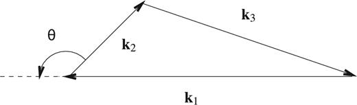
Generalized closed triangle configuration in |${\boldsymbol {k}}$| space that has been used for bispectrum estimation. This also shows the definition of the angle θ that we have used throughout this paper.
The four nested for loops in this algorithm determines all possible combinations of three components of |${\boldsymbol k}_1$| vector3 and one component of |${\boldsymbol k}_2$| vector. The other two components of |${\boldsymbol k}_2$| vector are determined by equations (3) and (4). All three components of |${\boldsymbol k}_3$| vector are determined using the closer of the triangle condition, i.e. |${\boldsymbol k}_1 +{\boldsymbol k}_2 +{\boldsymbol k}_3 = 0$|. Once all components of |${\boldsymbol k}_1$|, |${\boldsymbol k}_2$|, and |${\boldsymbol k}_3$| are determined, we take the product of three |$\Delta ({\boldsymbol k})$| corresponding to these three vectors, which will give us a complex number, as all |$\Delta ({\boldsymbol k})$|s are complex.
This particular approach to estimate bispectrum is very restrictive in nature. It does not allow any arbitrary bin width around |${\boldsymbol k}_2$| and |${\boldsymbol k}_3$| vectors. One can put a precise bin width around the |${\boldsymbol k}_1$| vector, but for a specific set of components of |${\boldsymbol k}_1$| and one component of |${\boldsymbol k}_2$|, other two components of |${\boldsymbol k}_2$| and all three components of |${\boldsymbol k}_3$| are determined precisely by equations (3) and (4), and the Kroneker delta function in (2). These equations of constraints do not allow any variation in the two components of |${\boldsymbol k}_2$| and all three components of |${\boldsymbol k}_3$|. This reduces the number of triangles contributing to every triangle bin, which affects more severely the triangle bins containing small |${\boldsymbol k}$| modes. One should thus be aware of the effect of the sample variance, which will be more significant at triangle bins containing small |${\boldsymbol k}$| modes, while interpreting the bispectrum estimated using this method.
3 SIMULATING THE REDSHIFTED 21-cm SIGNAL FROM THE EoR
We briefly describe here our method for simulating the redshifted 21-cm signal, which is identical to the approach of Mondal et al. (2017b). The three main steps in this method are – (a) generating the matter distribution at different redshifts using a particle-mesh N-body code (Bharadwaj & Srikant 2004; Mondal et al. 2015); (b) identifying collapsed haloes in that matter density field using a Friends-of-Friends (FoF) algorithm (Davis et al. 1985); and finally (c) generating an ionization field from the matter and halo distribution following an algorithm similar to the excursion set formalism of Furlanetto, Zaldarriaga & Hernquist (2004). Finally these ionization fields are converted into the redshifted 21-cm brightness temperature fields at their respective redshifts.
Our N-body simulation has a comoving volume of V = [215 Mpc]3 with 30723 grids of spacing 0.07 Mpc and a mass resolution of 1.09 × 10⁸ M⊙. To identify haloes from this matter distribution, we have set the criteria that a halo should have at least 10 dark matter particles (which implies a minimum halo mass of Mmin = 1.09 × 10⁹M⊙) and used a fixed linking length of 0.2 times the mean interparticle distance in our FoF halo finder.
We assume that the hydrogen traces the dark matter distribution. We also assume that the collapsed haloes host the sources of ionizing photons and the number of ionizing photons emitted by these sources are proportional to their host halo mass with a constant of proportionality Nion, which is a dimensionless parameter. The Nion is a combination of several unknown degenerate reionization parameters, such as, the star formation efficiency of the first galaxies, their UV photon production efficiency, and escape fraction of UV photons from them. To implement the excursion set formalism, we first map the matter and the ionizing photon density fields to a 3843 grid with spacing 0.56 Mpc. In this coarser grid (compared to the N-body grid), whether a grid point is neutral or ionized at a certain stage of reionization is determined by smoothing the hydrogen density and the ionizing photon density fields using spheres of different radii starting from a minimum radius of Rmin (the coarse grid spacing) to Rmfp. The Rmfp is another free parameter of our simulation, which represents the mean free path of the ionizing photons. A specific grid point in the simulation box is considered to be ionized if for any smoothing radius R (Rmin ≤ R ≤ Rmfp) the photon density exceeds the neutral hydrogen density at that grid point. This simulated ionization map or the corresponding neutral hydrogen density map is then converted into the 21-cm brightness temperature map. Our method of simulating the redshifted 21-cm signal is similar to that of Choudhury et al. (2009) and Majumdar et al. (2014). Note that we do not include redshift space distortions caused by peculiar velocities in our simulations, which in principle can have a significant effect on any estimator of the redshifted 21-cm signal from the EoR (Bharadwaj & Ali 2004; Barkana & Loeb 2005; Mao et al. 2012; Jensen et al. 2013a; Majumdar et al. 2013; Fialkov et al. 2015; Ghara et al. 2015b; Majumdar et al. 2016a,b). We plan to study this effect in a follow up work.
One can generate different reionization histories (i.e. mass averaged neutral fraction |$\bar{x}_{{{\rm H\,\small {I}}}}$| as a function of z) by varying parameters Nion and Rmfp. We use Rmfp = 20 Mpc for all redshifts which is consistent with the findings of Songaila & Cowie (2010) from the study of Lyman limit systems at low redshifts. We keep Nion = 23.21 fixed for all redshifts, so that |$\bar{x}_{{{\rm H\,\small {I}}}}\approx 0.5$| at z = 8. It also ensures that reionization ends at z ∼ 6 and we obtain Thomson scattering optical depth τ = 0.057, which is consistent with τ = 0.058 ± 0.012 reported by Planck Collaboration XVI (2016). The resulting reionization history is shown in Fig. 2. We generate five statistically independent realizations with the same reionization history to quantify the effect of cosmic variance on the signal bispectrum. Fig. 3 shows a visual representation of one slice of the signal cubes at three representative stages of reionization.
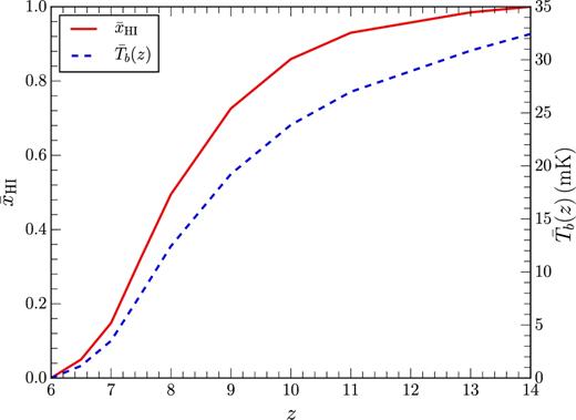
This shows the reionization history obtained from our simulations through the redshift evolution of average neutral fraction and average brightness temperature of the 21-cm signal.
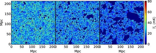
One realization of the real space 21-cm map at three representative stages of the reionization, |$\bar{x}_{{{\rm H\,\small {I}}}}= 0.86, \, 0.73,\, {\rm and}\, 0.49$| (from left to right), respectively.
4 MODELLING THE REDSHIFTED 21-cm BISPECTRUM FROM THE EoR
4.1 A toy model for H i fluctuation during the EoR
As we plan to use this toy model of |${{\rm H\,\small {I}}}$| bispectrum very extensively to interpret our simulated 21-cm bispectra, we discuss some of the important and relevant features of it in next few paragraphs. Bharadwaj & Pandey (2005) have discussed some of the shortcomings of this model when considered in the context of a realistic reionization scenario. First of all it assumes that the ionized spheres do not overlap with each other. This can be true at the very early stages of reionization when there are only a few ionized regions centred around the first ionizing sources. As reionization progresses, these ionized regions gradually grow in size and start overlapping with each other. Thus this model for the topology of ionization field is expected to break down during the later stages of the EoR or in other words when the average ionization fraction is relatively high (i.e. xi > 0.5). Another limitation of this model is that, it assumes that these ionized regions are randomly distributed in space, which is probably also not true as one would expect the ionized regions to be centred around the ionizing sources and these sources are expected to be located specifically in the matter density peaks. Thus one should expect a gravitational clustering in the distribution of the centre of these |${{\rm H\,\small {II}}}$| regions.
The other limitation of the above model is that it assumes all ionized regions at a specific stage of reionization to have the same radius R. This implies that the |${{\rm H\,\small {I}}}$| bispectrum (equation 11) for an equilateral triangle (i.e. k1 = k2 = k3) will be an oscillatory function of k1 with the first zero crossing appearing at k1R ≈ 4.49. As an example, for spheres of radius R = 10 Mpc this translates into first zero crossing to appear at k1 ≈ 0.45 Mpc−1. However, various realistic simulations of reionization predict that the ionized regions at a certain stage of reionization will be of different shapes and volume (see e.g. Zahn et al. 2007; Friedrich et al. 2011; Majumdar et al. 2014; Iliev et al. 2015, etc.). Some recent studies (see e.g. Furlanetto & Oh 2016; Bag et al. 2018) even suggest that the ionized regions are not spherical but rather filamentary in shape. Additionally, there is no such characteristic ‘size’ that can be assigned to the ionized regions as they percolate with each other even at very early stages of the EoR. As a first-order improvement of the Bharadwaj & Pandey (2005) model, we propose a phenomenological model for the |${{\rm H\,\small {I}}}$| bispectrum where we assume that |$B_{{{\rm H\,\small {I}}}}({\boldsymbol k}_1, {\boldsymbol k}_2, {\boldsymbol k}_3)\propto - \sum _{a} W(k_1 R_a) W(k_2 R_a) W(k_3 R_a)$|. Under this model Ras are drawn from a distribution rather than having a fixed value. Note that, though this modified toy model is inspired by the model of Bharadwaj & Pandey (2005) (i.e. equation 11) but is not a direct extension or generalization of the above.
Fig. 4 shows bispectra for a set of triangle configurations for the two models of |${{\rm H\,\small {I}}}$| fluctuations introduced earlier. The top panel of this figure shows the |${{\rm H\,\small {I}}}$| bispectra for equilateral triangles as a function of k1. The solid line corresponds to the model with a fixed bubble radius (R = 10 Mpc). As expected the bispectrum for this model is an oscillatory function of k1 and its first zero crossing appears at k1 ≈ 0.45 Mpc−1. The dashed, dash–dotted, and dotted lines represent models with a uniform (with R in the range 0.56 Mpc ≤ R ≤ 25 Mpc), log-normal (with parameters μ = 2.3 and σ = 0.6), and Gaussian (with parameters μ = 10 Mpc and σ = 3.0) bubble size distributions. We have chosen the parameter values for the log-normal and the Gaussian bubble size distributions such that both of the distributions (corresponding histograms not shown here) peak around R ≈ 10 Mpc. In contrast with the bispectrum for fixed R, the bispectra for models with a distribution in Ra turn out to be a power law like smooth functions of k1. For the uniform and Gaussian bubble distribution of R we do not observe any zero crossing in the bispectra. The bispectrum for the log-normal distribution in R shows a zero crossing at significantly large k1 mode (k1 ∼ 4.00 Mpc−1), possibly reflects the presence of a large number of smaller R values in this distribution. The other main features of the bispectrum from this modified toy model, some of which are same as the model with fixed bubble radius, are the following: (a) this bispectrum is negative; (b) it remains almost constant as a function of k, for a k range corresponding to significantly large length scales; (c) the amplitude of the bispectrum rapidly falls off and shows almost a power law like feature for 0.1 Mpc−1 < k ≲ 4.00 Mpc−1.
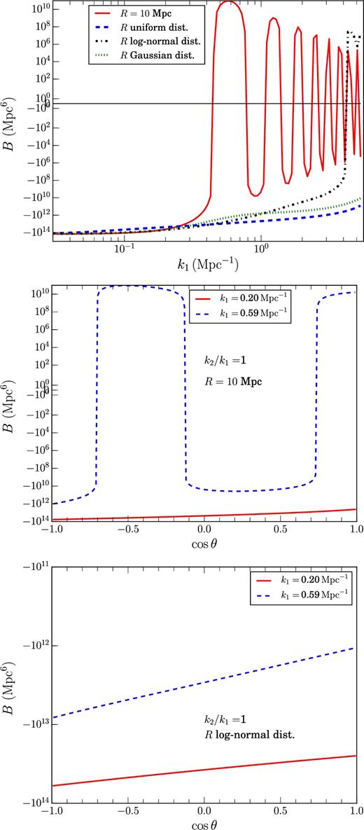
Top panel: Model bispectrum (in arbitrary units) for equilateral triangles as function of k. Solid, dashed, dash–dotted, and dotted lines represent the model bispectra for a fixed bubbles radius R = 10 Mpc, uniformly distributed bubble radii in the range 0.56 Mpc ≤ R ≤ 25 Mpc, log-normal bubble radii distribution with μ = 2.3 and σ = 0.3, Gaussian bubble radii distribution with Rmean = 10 Mpc and σ = 3.0, respectively. Central panel: Model bispectrum for isosceles triangles (k2/k1 = 1) as a function of cos θ. The model bispectra shown here is for a fixed bubbles radius R = 10. Solid and dashed lines represent bispectra for two different values of k1 (0.20 and 0.59 Mpc−1, respectively). Bottom panel: Same as the central panel but for the model with log-normal bubble radii distribution. Note that in all three panels, the y-axis is shown in log scale, using the symlog function of matplotlib in python, which is linear in between −1 and 1 and log in the rest of the range.
We expect some of these features of the model |${{\rm H\,\small {I}}}$| bispectra that are observed for the equilateral triangles to hold true for other triangle configurations as well. To demonstrate it further, we show the bispectrum for isosceles triangles (i.e. k1 = k2) in the central and bottom panels of Fig. 4 for models with a fixed bubble radius and with a log-normal distribution in bubble sizes, respectively. We choose two fixed k1 values (k1 = 0.20 and 0.59 Mpc−1) and plot the bispectrum as a function of cos θ (defined by equation 4). It is apparent from Fig. 1 that cos θ ∼ −1 represents ‘squeezed’ limit of triangles and cos θ ∼ 1 represents ‘stretched’ limit of triangles. Further, cos θ = −0.5 in this plot correspond to equilateral triangles. For the |${{\rm H\,\small {I}}}$| fluctuation model with a fixed bubble radius (central panel of Fig. 4), with triangles consisting of sufficiently large length scales (k1 = 0.20 Mpc−1) the bispectrum (solid red line) is negative and a smooth function of cos θ. It attains maximum amplitude at the ‘squeezed’ limit of triangles (cos θ ∼ −1) and minima at the ‘stretched’ limit (cos θ ∼ 1). Note that the value of k3 for this type of triangles, in the entire cos θ range stays below k3 ≤ 0.40 Mpc−1, which is smaller than the first zero crossing k mode for this |${{\rm H\,\small {I}}}$| fluctuation model. This ensures that the model bispectrum is a smooth function of cos θ at large length scales. However, the bispectrum for k1 = 0.59 Mpc−1 (dashed blue line) becomes an oscillatory function of cos θ as all three k modes involved in this type of triangles are beyond the first zero crossing limit. The bispectrum for our modified model with a log-normal bubble size distribution, turns out to be a smooth function of cos θ for both k1 = 0.20 and 0.59 Mpc−1 (bottom panel of Fig. 4), provided that the range of the bubble radii has been sampled sufficiently enough that the oscillations due to different bubble radii wash out each other. This model also shows a larger bispectrum amplitude at smaller k1 modes and for any fixed k1 mode bispectrum amplitude is maximum for cos θ ∼ −1 and minimum for cos θ ∼ 1.
In the next few sections of this paper we will observe that the behaviour of the bispectrum estimated from the simulated 21-cm signal shows behaviour that are similar to this model |${{\rm H\,\small {I}}}$| bispectrum for a wide variety of triangles. We thus discuss and interpret the 21-cm bispectrum estimated from our simulations in the light of this particular modified model of |${{\rm H\,\small {I}}}$| bispectrum.
5 RESULTS
The bispectrum estimator described in Section 2 has been tested extensively for different |${\boldsymbol k}$|-triangle configurations using a matter density field (from a particle-mesh N-body simulation) and a toy non-Gaussian field made of randomly distributed non-overlapping ionized bubbles in a uniformly dense neutral medium in Watkinson et al. (2017). Watkinson et al. (2017) has also compared its performance against another estimator of bispectrum. We thus do not repeat those tests in this paper and direct the interested reader to Watkinson et al. (2017) for a detailed description of these tests.
While studying the bispectrum for a highly non-Gaussian field such as the EoR 21-cm signal, one can in principle consider a large variety of triangle configurations using different values of the wavenumber triplets |${\boldsymbol k}_1, {\boldsymbol k}_2, \,{\rm and}\, {\boldsymbol k}_3$|. Bispectra for different unique |${\boldsymbol k}$|-triangle configurations can potentially probe different unique non-Gaussian features present in the signal. We can vary the |${\boldsymbol k}$|-triangle configuration for our analysis using the two equation of constraints (equations 3 and 4) of our algorithm. To keep the length of our analysis within a reasonable limit, we choose a set of triangle configurations which probes the different extremes of the possible triangle configurations. Following equation (3), we choose four different values for the ratio k2/k1, namely n = 1, 2, 5, and 10. For each value of n we vary cos θ within the range −1 ≤ cos θ ≤ 1 with steps of Δcos θ = 0.01. Compared to power spectrum, the binning for bispectrum can be tricky, as instead of only one k mode here we have three k modes associated with each bispectrum value. We bin our bispectrum estimates in the following way: for a specific value of n and cos θ we divide the entire k1 range [kmax = π/(grid spacing) = 5.61 Mpc−1 to kmin = 2π/(box size) = 0.03 Mpc−1] into 15 logarithmic bins and label each bin with the value of k1 at the centre of that bin. Note that the effective mean value of k1 vector in each such bin can be different from central value of the bin. Throughout this paper, unless otherwise stated, we show the bispectrum as a function of (k1, n, cos θ). Also note that for a specific triangle type we consider all possible orientations of the |${\boldsymbol k}_1$| vector (and subsequent orientations of the other two |${\boldsymbol k}$|s) in the k-space and thus all of the bispectra that we describe here are essentially spherically averaged in k-space.
5.1 Equilateral triangles
The first obvious triangle configuration to study is the equilateral triangle (i.e. k1 = k2 = k3). Just as the power spectrum, which can be expressed as a function of the amplitude of |${\boldsymbol k}$| alone, the equilateral bispectrum can also be expressed as a amplitude of just |${\boldsymbol k}_1$|, as all arms of the triangle have the same amplitude. It will capture the correlation present in the signal between three different point in k space equidistant from each other. Fig. 1 suggests that for equilateral triangles cos θ = −0.5. However, as discussed in Section 2, due to the very restrictive nature of the algorithm (which does not allow a finite width in the cos θ bin but rather estimates bispectra for very precise sharp values of cos θ) that we have employed to estimate bispectrum, it will be prone to sample variance, specifically for triangles involving small k modes. To reduce the effect of this sample variance for equilateral triangle configurations, we average over all bispectra estimated within the cos θ range −0.52 ≤ cos θ ≤ −0.48.
The top panel of Fig. 5 shows the equilateral bispectra estimated at four representative stages of the EoR (in terms of |$\bar{x}_{{{\rm H\,\small {I}}}}$| values) as a function of k1. The error bars on the curves in this figure represent the 1σ uncertainty estimated from five statistically independent realizations of the simulated signal. For the sake of clarity we show error bars only for a single value of |$\bar{x}_{{{\rm H\,\small {I}}}}$| (namely 0.73). The estimated bispectrum becomes sample variance dominated for k1 bins corresponding to k1 ≲ 0.1 Mpc−1 as the number of closed triangles becomes significantly small at these values due to the very restrictive nature of our estimator. Thus we do not show the bispectrum beyond k1 ≲ 0.1 Mpc−1. For a better understanding of the evolution of B with |$\bar{x}_{{{\rm H\,\small {I}}}}$| at different length scales we also plot B as a function of |$\bar{x}_{{{\rm H\,\small {I}}}}$| for three representative k1 values (k1 = 0.20, 0.58 and 1.18 Mpc−1) in the central panel of Fig. 5.
![Top panel: Bispectra for equilateral triangles as a function of k at four representative stages ($\bar{x}_{{{\rm H\,\small {I}}}}= 0.86, \, 0.73, \, 0.49,\, {\rm and}\, 0.32$) of the EoR. The error bars represent 1σ uncertainty estimated from the five statistically independent realizations of the simulated signal. For clarity, we show error bars only for one $\bar{x}_{{{\rm H\,\small {I}}}}$ value. Central panel: 21-cm bispectrum for equilateral triangles as a function of $\bar{x}_{{{\rm H\,\small {I}}}}$ at three representative length scales (k = 0.20, 0.58, and 1.18 Mpc−1). Bottom panel: Eight component (following equation 7) bispectra estimated from the simulations as a function of $\bar{x}_{{{\rm H\,\small {I}}}}$ for k = 0.58 Mpc−1 (x represents $x_{{{\rm H\,\small {I}}}\,}$ field and Δ represents matter density field). This also shows the sum of all eight components and two main component bispectra (BΔΔΔ and Bxxx), separately, along with the 21-cm bispectrum [$B/\overline{T}^3_b(z)$] for comparison. Note that in all three panels, the y-axis is shown using the symlog function of matplotlib, which is linear in between −1 and 1 and log in the rest of the range.](https://oup.silverchair-cdn.com/oup/backfile/Content_public/Journal/mnras/476/3/10.1093_mnras_sty535/1/m_sty535fig5.jpeg?Expires=1749936724&Signature=SiPD9AFOKEw8AtVYSY9mCVgt~RJQwQMKOgU73SvfmI4X5RmwwC7akajULE9BgQTvUlRvcBBbGrE08KCbb2HGBKyZuiUJrUVYYghCtAoZmjxE5smFnoMCnUU-veh~oQ~6Y6X-rUOv5myFibGxIpJBTteTZ9gayXWhmGJh3rk2rYzbb4lBtjQuhbVzz1WbPMTpk5XY652Dl-tBNUccychu8xAVAKvU-JwhuWPgpIT83gINV0lh1-Q88a8zD0KgUETcOw5K03-sA0vSG1LOs88Fb2IQ1eGru6gjgIglIvsvNyTifVHux9UMD3f~ez3L3FGWs7wkbWNvLYbfF7y3WW0eaw__&Key-Pair-Id=APKAIE5G5CRDK6RD3PGA)
Top panel: Bispectra for equilateral triangles as a function of k at four representative stages (|$\bar{x}_{{{\rm H\,\small {I}}}}= 0.86, \, 0.73, \, 0.49,\, {\rm and}\, 0.32$|) of the EoR. The error bars represent 1σ uncertainty estimated from the five statistically independent realizations of the simulated signal. For clarity, we show error bars only for one |$\bar{x}_{{{\rm H\,\small {I}}}}$| value. Central panel: 21-cm bispectrum for equilateral triangles as a function of |$\bar{x}_{{{\rm H\,\small {I}}}}$| at three representative length scales (k = 0.20, 0.58, and 1.18 Mpc−1). Bottom panel: Eight component (following equation 7) bispectra estimated from the simulations as a function of |$\bar{x}_{{{\rm H\,\small {I}}}}$| for k = 0.58 Mpc−1 (x represents |$x_{{{\rm H\,\small {I}}}\,}$| field and Δ represents matter density field). This also shows the sum of all eight components and two main component bispectra (BΔΔΔ and Bxxx), separately, along with the 21-cm bispectrum [|$B/\overline{T}^3_b(z)$|] for comparison. Note that in all three panels, the y-axis is shown using the symlog function of matplotlib, which is linear in between −1 and 1 and log in the rest of the range.
The first obvious observation that one can make from these plots is that the bispectrum is non-zero and for smaller k modes its amplitude increases with increasing global ionization fraction. This establishes the fact that the 21-cm signal is highly non-Gaussian in nature and its degree of non-Gaussianity increases with the progress of reionization. The other important and obvious feature of the bispectrum for the equilateral triangle configuration is that it has a negative sign for a large range of k1 values (0.1 Mpc−1 ≲ k1 ≲ 3.0 Mpc−1), during almost the entire period of reionization. This is in agreement with the predictions from the toy model of |${{\rm H\,\small {I}}}$| fluctuations discussed in Section 4.1 and shown in the top panel of Fig. 4. We note that this particular feature of the bispectrum was not observed in the analysis done by Yoshiura et al. (2015) and Shimabukuro et al. (2016, 2017). This is due to the fact that they define their bispectrum estimator as the absolute value (or modulus) of the product of three complex |$\Delta ({\boldsymbol k})$|s, i.e. their estimator is essentially |$\langle \lbrace {\Re }[\Delta ({\boldsymbol k}_1) \Delta ({\boldsymbol k}_2) \Delta ({\boldsymbol k}_3)]^2 + {\Im }[\Delta ({\boldsymbol k}_1) \Delta ({\boldsymbol k}_2) \Delta ({\boldsymbol k}_3)]^2\rbrace ^{1/2} \rangle$|. Note that, they have an imaginary component in their bispectrum estimation which appears simply because for a bispectrum estimation they consider closed triangles from only one half of the k-space. As we discuss in Section 2 that when triangles from the entire k-space is considered this imaginary component will become exactly zero. Therefore the imaginary component does not have any physical significance. Further, it is clear that, by construction their estimator will always be positive and will not be able to capture the sign of the bispectrum or any change in its sign either. The sign of the bispectrum is an important feature of the signal and we will discuss it further in the context of other |${\boldsymbol k}$|-triangle configurations in the later part of this paper.
A further visual inspection of the different B(k1) curves in the top panel of Fig. 5 reveals that B(k1) shows a power law like decline in amplitude with increasing k1 for 0.1 Mpc−1 ≲ k1 ≲ 2.0 Mpc−1 during almost the entire period of reionization, which is again in agreement with the toy model of Section 4.1. For the later stages of reionization, B(k1) shows a further sharp decline beyond k1 ≳ 2.0 Mpc−1 and even reaches positive values at |$\bar{x}_{{{\rm H\,\small {I}}}}\le 0.5$| for k1 ≳ 3.0 Mpc−1. The central panel of the Fig. 5 further shows that for triangles involving large length scales, i.e. small k1 values (k1 = 0.20 Mpc−1) the amplitude of B(k1) increases significantly with the decreasing |$\bar{x}_{{{\rm H\,\small {I}}}}$| (or increasing xi) until reionization is half way through (i.e. |$\bar{x}_{{{\rm H\,\small {I}}}}\sim 0.5$|). The toy model also predicts an increase in amplitude with the increasing xi. For |$\bar{x}_{{{\rm H\,\small {I}}}}< 0.5$| the amplitude of B(k1) gradually decreases. Note that this is also the regime during the EoR when the overlap of different ionized regions becomes significant in a realistic ionization topology and the actual shapes of the ionized regions depart further from that of an ideal sphere. Thus it is unlikely that the toy model of individual non-overlapping spherical ionized regions will capture the true nature of the bispectrum in this regime. For triangles involving intermediate (k1 = 0.58 Mpc−1) and large (k1 = 1.18 Mpc−1) k modes the increase in amplitude is observed until |$\bar{x}_{{{\rm H\,\small {I}}}}\sim 0.7$| and for the later stages of reionization the amplitude gradually decreases. The next simulation snapshot that we have available for |$\bar{x}_{{{\rm H\,\small {I}}}}$| values below |$\bar{x}_{{{\rm H\,\small {I}}}}= 0.32$| is at |$\bar{x}_{{{\rm H\,\small {I}}}}\approx 0.15$|. We find that the amplitude of the bispectrum goes down significantly for |$\bar{x}_{{{\rm H\,\small {I}}}}\approx 0.15$| and the sample variance for our bispectrum estimate is also very high at this stage. We therefore do not show the results for any neutral fraction values below |$\bar{x}_{{{\rm H\,\small {I}}}}< 0.32$|.
The bottom panel of Fig. 5 shows the evolution of the various component bispectra (against |$\bar{x}_{{{\rm H\,\small {I}}}}$|, for k1 = 0.58 Mpc−1), estimated from the matter density and |$x_{{{\rm H\,\small {I}}}\,}$| fields that are used to simulate the 21-cm signal (see equation 7). In this figure we have scaled the 21-cm bispectrum with |$1/\overline{T}^3_{{\rm b}}(z)$| to keep its dimension similar to all the component bispectra. It is evident from this plot that the major component contributing to the 21-cm bispectrum for equilateral triangles (solid red line with error bars) for almost the entire period of reionization is the neutral fraction bispectrum (solid blue line with diamonds). We also observe that the sum of all of the eight components of bispectrum (black dotted curve) does not follow the evolution of the 21-cm bispectrum, even qualitatively. However, the sum of the neutral fraction and density bispectra (cyan dashed line) does follow the evolution of the 21-cm bispectrum in terms of its shape, if not exactly in terms of its amplitude, especially during the intermediate and late stages of reionization. We observe a similar behaviour, i.e. the 21-cm bispectrum closely following the |$x_{{{\rm H\,\small {I}}}\,}$| field bispectrum, for a wide range of length scales i.e. 0.20 Mpc−1 ≤ k1 ≤ 1.18 Mpc−1 (not shown in the figure). The |$x_{{{\rm H\,\small {I}}}\,}$| bispectrum, which is the main contributor to the 21-cm bispectrum for this type of triangle, also follows (at least qualitatively) the shape and evolution predicted by the toy model of |$x_{{{\rm H\,\small {I}}}\,}$| fluctuations discussed in Section 4.1. This further establishes that this toy model is a reasonably good tool for interpreting the qualitative behaviour of the 21-cm bispectrum, at least for this type of triangles, as this type of bispectra is sensitive to the fluctuations generated by the distribution of |${{\rm H\,\small {II}}}$| regions. However, the sum of all eight components of equation (7) does not follow the 21-cm bispectrum (even qualitatively) which can be attributed to the fact that the equation (7) has been obtained under the linear approximation limit of the Fourier transform of equation (5). If one considers that the higher order terms in density fluctuations and neutral fraction also have significant contributions to the 21-cm signal, then there will be many higher order component bispectra (e.g. BΔx(Δx), BΔ(Δx)(Δx), ...) contributing to the 21-cm bispectrum. Thus a correction to the equation (7) by including higher order contributions of two constituent fields may provide us a more accurate model for the EoR 21-cm bispectrum. A similar model in the context of the EoR 21-cm power spectrum has been discussed in Lidz et al. (2007) through their equation (2) and (3). We plan to study the effectiveness of such an higher order model in the context of interpreting the EoR 21-cm bispectrum in a future follow-up work.
5.2 Evolution of the 21-cm signal in P(k) − B(k, k, k) space
Since the spherically averaged power spectrum and the bispectrum for equilateral triangles are two independent but complementary measures of the 21-cm signal and both can be represented as a function of the amplitude of just one wavenumber k, one can thus visualize the evolution of the 21-cm signal as a trajectory in the phase space4 of P(k) − B(k, k, k). In Fig. 6 we show the evolution of the signal in such a phase space diagram for two representative values of k (k = 0.20 and 0.58 Mpc−1). As, for these two wavenumbers, the B stays negative for the entire range of |$\bar{x}_{{{\rm H\,\small {I}}}}$| values that we consider, we plot −ℜ[B] instead of B in this figure for a better understanding of the signal evolution. A close inspection of Fig. 6 reveals many similarities in the qualitative behaviour of the signal trajectories at different length scales along with some differences. For both length scales, the signal initially shows a rise in amplitude in the bispectrum but a decline in amplitude in the power spectrum. The power spectrum reaches a minimum around |$\bar{x}_{{{\rm H\,\small {I}}}}\approx 0.85$| beyond which it starts to grow in amplitude with decreasing |$\bar{x}_{{{\rm H\,\small {I}}}}$|. Both power spectra and bispectra continues to grow in amplitude until the trajectory reaches a turn-around point. For relatively larger length scales (i.e. k = 0.20 Mpc−1, top panel of Fig. 6) this turn-around point appears at |$\bar{x}_{{{\rm H\,\small {I}}}}\approx 0.50$| and for intermediate length scales (i.e. k = 0.58 Mpc−1, bottom panel of Fig. 6) it appears at |$\bar{x}_{{{\rm H\,\small {I}}}}\approx 0.70$|. Beyond this turn-around point both power spectra and bispectra decrease in amplitude with decreasing neutral fraction. The bispectrum decreases relatively sharply compared to the power spectrum. If different reionization source models lead to different 21-cm topologies, one would then expect their 21-cm signal trajectories in P(k) − B(k, k, k) phase space to be different from each other. These trajectories provide us a consolidated view of the signal by combining both power spectrum and bispectrum. Each of which is expected to probe a different characteristic of the signal. Similarly, one would expect a joint MCMC analysis (or a similar sort of likelihood analysis) of power spectrum and bispectrum to provide a more robust constraint on the reionization model parameters compared to the similar MCMC analysis done with a single signal estimator (either power spectrum or bispectrum) alone (e.g. Greig & Mesinger 2015, 2017; Shimabukuro et al. 2017; Schmit & Pritchard 2018, etc.).
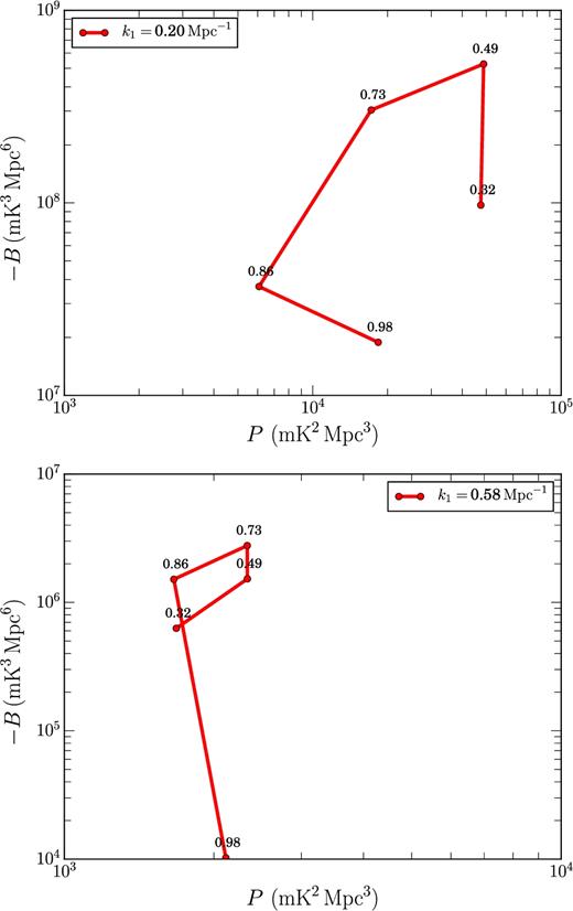
Signal trajectories in the P(k) − B(k, k, k) phase space for k = 0.20 and 0.58 Mpc−1. Note that here we show −B instead of B. The corresponding values of |$\bar{x}_{{{\rm H\,\small {I}}}}$| have been printed on the respective points of the trajectories.
5.3 Isosceles triangles
The first-order generalization of equilateral triangles (n = 1 and cos θ = −0.5) will lead to isosceles triangles (n = 1 and −1 ≤ cos θ ≤ 1). Compared to equilateral triangles, which show correlations in the signal for three equidistant points in the Fourier space, isosceles triangles will have two equal length k arms and the third arm will be different in length (determined by the respective cos θ value). Thus the bispectrum for isosceles triangles will effectively show the correlation in the signal between two different k modes. Fig. 7 shows the isosceles bispectra for the simulated 21-cm signal at different stages of reionization as a function of cos θ.
![21-cm bispectra for isosceles triangles as a function of cos θ at different stages of reionization marked by their corresponding $\bar{x}_{{{\rm H\,\small {I}}}}$ values. Different panels show bispectra for different values of k1 (k1 = 0.20, 0.29, 0.58, 1.18, and 1.67 Mpc−1). The entire cos θ range has been divided into 20 linearly spaced bins. Points in each bispectrum curve represent the mid-point of the corresponding cos θ bin. The error bars shown on the bispectrum for one $\bar{x}_{{{\rm H\,\small {I}}}}$ value represent 1σ uncertainty estimated from the five statistically independent realizations of the signal. To have a better understanding of all the length scales involved in the bispectrum estimation, we also show the amplitude of ${\boldsymbol k}_3$ as a function of cos θ through the dotted black curve in all panels (refer to the right y-axis in each panel to evaluate the k3 curve at a specific value of cos θ). The bottom right panel shows the two major component bispectra (matter density – BΔΔΔ and neutral fraction – Bxxx) and their sum as functions of cos θ for k1 = 0.58 Mpc−1 and $\bar{x}_{{{\rm H\,\small {I}}}}= 0.49$. We also show the corresponding 21-cm bispectrum [$B/\overline{T}^3_{\rm b}(z)$] in the same panel for comparison. Note that in all panels the entire left y-axis is shown in logarithmic scale, except the range −1 to 1, where the scale is linear. The right y-axis is shown in linear scale in all panels.](https://oup.silverchair-cdn.com/oup/backfile/Content_public/Journal/mnras/476/3/10.1093_mnras_sty535/1/m_sty535fig7.jpeg?Expires=1749936724&Signature=12sSPyvE5icWd0PnlwsmT4rFhU4sNsHSdb64bJcrNYuFttWpLVaEnmIu63uYS9izx9N4Ct4Fwg87u~Ou-RAILhVp9R-obliKGikyRh96coYXuvTqE3lEfWolZ47GBlfKyavY~-8z7ls7WJQUrwK5jX17NjpK1hkqUa7OEyM6XtyjTIWCpGI3ALySBjiCVIPiHMFbi4Lv2OtRfWGDVXSUTJ7hfMT~lMeXktA78szCIBdgdZ8yrhNHJn3IuDS9KSxJhWpD10Po08t~4iDq~LWtJ0REPuW0dfPF4Gja6yaS0Z7oPhYukiJGhexzxvkAqHiLafJUZbl6ckWRZmaLkIqRxQ__&Key-Pair-Id=APKAIE5G5CRDK6RD3PGA)
21-cm bispectra for isosceles triangles as a function of cos θ at different stages of reionization marked by their corresponding |$\bar{x}_{{{\rm H\,\small {I}}}}$| values. Different panels show bispectra for different values of k1 (k1 = 0.20, 0.29, 0.58, 1.18, and 1.67 Mpc−1). The entire cos θ range has been divided into 20 linearly spaced bins. Points in each bispectrum curve represent the mid-point of the corresponding cos θ bin. The error bars shown on the bispectrum for one |$\bar{x}_{{{\rm H\,\small {I}}}}$| value represent 1σ uncertainty estimated from the five statistically independent realizations of the signal. To have a better understanding of all the length scales involved in the bispectrum estimation, we also show the amplitude of |${\boldsymbol k}_3$| as a function of cos θ through the dotted black curve in all panels (refer to the right y-axis in each panel to evaluate the k3 curve at a specific value of cos θ). The bottom right panel shows the two major component bispectra (matter density – BΔΔΔ and neutral fraction – Bxxx) and their sum as functions of cos θ for k1 = 0.58 Mpc−1 and |$\bar{x}_{{{\rm H\,\small {I}}}}= 0.49$|. We also show the corresponding 21-cm bispectrum [|$B/\overline{T}^3_{\rm b}(z)$|] in the same panel for comparison. Note that in all panels the entire left y-axis is shown in logarithmic scale, except the range −1 to 1, where the scale is linear. The right y-axis is shown in linear scale in all panels.
For relatively small |${\boldsymbol k}$|-triangles (i.e. k1 = k2 = 0.20 Mpc−1, top left panel of Fig. 7) and during the early and the intermediate stages of reionization (|$\bar{x}_{{{\rm H\,\small {I}}}}= 0.86$| and 0.73) the 21-cm bispectrum is negative. At these stages of reionization, the amplitude of the bispectrum is maximum in the ‘squeezed’ limit (cos θ ∼ −1) and it decreases with the increasing cos θ (as one moves towards the ‘stretched’ limit). This decrease is rapid for −1 ≤ cos θ ≤ −0.5 (while k3 stays within the range 0.05 Mpc−1 ≤ k3 ≤ 0.20 Mpc−1) and relatively slow for the rest of the cos θ range (i.e. 0.20 Mpc−1 ≤ k3 ≤ 0.40 Mpc−1). The overall amplitude of B also increases with decreasing neutral fraction and this behaviour holds true for average neutral fraction values as low as |$\bar{x}_{{{\rm H\,\small {I}}}}\approx 0.50$| and for cos θ values up to ≈0.8 (i.e. k3 ≤ 0.40 Mpc−1). Most of these characteristics qualitatively follow the predictions of our toy model in Section 4.1 (see bottom panel of Fig. 4).
As we move towards triangles with slightly larger k values (e.g. k1 = k2 = 0.29 Mpc−1, top right panel of Fig. 7) we observe that the increase in the overall amplitude of B with decreasing |$\bar{x}_{{{\rm H\,\small {I}}}}$| predicted by our toy model breaks down. We observe that for k1 = 0.29 Mpc−1 the bispectrum for |$\bar{x}_{{{\rm H\,\small {I}}}}= 0.49$| becomes equal or smaller in amplitude than the bispectrum for |$\bar{x}_{{{\rm H\,\small {I}}}}= 0.73$| for cos θ ≥ 0 (i.e. k3 ≥ 0.40 Mpc−1). This deviation of the signal bispectrum from the toy model prediction continues even in the later stages of reionization (not shown in this panel of Fig. 7). Note that we do not show the bispectrum for |$\bar{x}_{{{\rm H\,\small {I}}}}= 0.32$| in the top panels of Fig. 7 (i.e. for k1 = 0.20 and 0.29 Mpc−1) as it has a large dynamic range compared to the bispectrum for other neutral fractions. We discuss the characteristics of bispectrum for |$\bar{x}_{{{\rm H\,\small {I}}}}= 0.32$| corresponding to these k1 modes later in this section.
As we take our analysis to triangles with intermediate and large values of k1 (k1 = k2 = 0.58, 1.18, and 1.67 Mpc−1) we observe several other interesting features in the bispectrum. For k1 = 0.58 Mpc−1 (central left panel of Fig. 7), the ‘squeezed’ limit (i.e. cos θ ≈ −1, k3 ≈ 0.20 Mpc−1) triangles follow the trend of rise in bispectrum amplitude with decreasing |$\bar{x}_{{{\rm H\,\small {I}}}}$| up to |$\bar{x}_{{{\rm H\,\small {I}}}}\ge 0.7$|. Beyond this, we observe a gradual reversal in this trend for lower neutral fraction values. At these stages of reionization the signal amplitude tends to decrease with decreasing |$\bar{x}_{{{\rm H\,\small {I}}}}$| values.
The most interesting feature that we observe for triangles with k1 = 0.58 Mpc−1 is a change of sign in the bispectrum (from negative to positive) as we approach the ‘stretched’ limit of these triangles. This change in sign is observed first for |$\bar{x}_{{{\rm H\,\small {I}}}}= 0.73$| prominently around cos θ ≈ 1 (though the actual transition happens somewhere in between 0.7 ≲ cos θ ≲ 0.9, i.e. 1.08 ≲ k3 ≲ 1.16 Mpc−1, but difficult to ascertain the exact point of transition due to the large cosmic variance in this range). Interestingly enough, during the later stages of reionization this transition (change in sign) happens at gradually lower values of cos θ. For |$\bar{x}_{{{\rm H\,\small {I}}}}= 0.32$| the B becomes positive at around cos θ ≈ 0.5 (i.e. k3 ≈ 1.0 Mpc−1), beyond which it remains positive. To confirm these features are real and not due to any numerical artefact in our algorithm, we have used the bispectrum estimator of Watkinson et al. (2017) and obtained the same results. We have observed similar features in the 21-cm bispectrum for k1 = 0.20 and 0.29 Mpc−1 (not shown in these figures) at very late stages of reionization (|$x_{{{\rm H\,\small {I}}}\,} = 0.32$|).
The fact that this change of sign in B is a systematic behaviour, and is strongly dependent on the stage of reionization (i.e. |$\bar{x}_{{{\rm H\,\small {I}}}}$|) and the length scales involved for the bispectrum estimation, becomes very apparent as one observes the results for triangles with k1 = 1.18 and 1.67 Mpc−1 (central right and bottom left panels of Fig. 7). As one approaches triangles with larger k1 values (which implies larger k3 amplitudes as well), one observes this sign reversal to occur at very early stages of reionization (|$\bar{x}_{{{\rm H\,\small {I}}}}= 0.86$|) and at even lower values of cos θ. For k1 = 1.18 Mpc−1 it occurs at cos θ ≈ 0.5 (i.e. k3 ≈ 2.10 Mpc−1) for |$\bar{x}_{{{\rm H\,\small {I}}}}= 0.86$| and at cos θ ≈ 0.3 (i.e. k3 ≈ 1.95 Mpc−1) for |$\bar{x}_{{{\rm H\,\small {I}}}}= 0.32$|. Similarly, for k1 = 1.67 Mpc−1 it occurs at cos θ ≈ 0.3 (i.e. k3 ≈ 2.8 Mpc−1) for |$\bar{x}_{{{\rm H\,\small {I}}}}= 0.86$| and at cos θ ≈ 0 (i.e. k3 ≈ 2.4 Mpc−1) for |$\bar{x}_{{{\rm H\,\small {I}}}}=0.32$|. Further, for the triangle configurations with the largest k1 amplitude we observe that the overall amplitude of the bispectrum (irrespective of its sign) gradually decreases with decreasing |$\bar{x}_{{{\rm H\,\small {I}}}}$|. We also observe that for triangles with these two large k1 values, during the later stages of reionization (|$\bar{x}_{{{\rm H\,\small {I}}}}\le 0.5$|), the bispectrum at the ‘squeezed’ limit (cos θ ≈ −1) also becomes positive.
To get some physical insight in the trends for isosceles triangles, we plot in the bottom right panel of Fig. 7 the two main component bispectra: BΔΔΔ and Bxxx, and the sum of these two components, along with the 21-cm bispectra at |$\bar{x}_{{{\rm H\,\small {I}}}}= 0.49$| for k1 = 0.58 Mpc−1. We choose this set of k1 and |$\bar{x}_{{{\rm H\,\small {I}}}}$| values because this combination of k1 and |$\bar{x}_{{{\rm H\,\small {I}}}}$| clearly shows most of the main features of the 21-cm isosceles bispectrum that we have described. The above panel shows that for most of the cos θ range (−1 ≲ cos θ ≲ 0.5, i.e. 0.2 Mpc−1 ≲ k3 ≲ 1 Mpc−1) where it is negative, the 21-cm bispectrum very closely follows Bxxx. This is also the cos θ range where the shape of the B curve as a function of cos θ follows the prediction from our toy model for the |$x_{{{\rm H\,\small {I}}}\,}$| fluctuation bispectrum (see bottom panel of Fig. 4). Note that the k modes that form closed triangles within this cos θ range are either small or intermediate in amplitude (0.2 Mpc−1 ≲ k ≲ 1 Mpc−1). The contribution from BΔΔΔ (which is, as expected, always positive in the entire cos θ range) is negligible compared to Bxxx at this range, as their sum (BΔΔΔ + Bxxx) also largely follows the |$x_{{{\rm H\,\small {I}}}\,}$| bispectrum. During the early and intermediate stages of the EoR (i.e. |$\bar{x}_{{{\rm H\,\small {I}}}}\gtrsim 0.5$|), the 21-cm signal fluctuations involving these k modes will be dominated by the size distribution of the individual isolated ionized regions. A simplified version of which formulates our toy model for |$x_{{{\rm H\,\small {I}}}\,}$| fluctuations. Thus one would expect the toy model to be able to qualitatively describe the 21-cm as well as the |$x_{{{\rm H\,\small {I}}}\,}$| bispectrum in this regime.
As reionization progresses the ionization topology deviates from this simplified model. A recent study by Bag et al. (2018) (done with an almost identical simulation as the one presented here; see also Furlanetto & Oh 2016) suggests that most of the isolated ionized regions percolate and leads to a single ionized region as early as |$\bar{x}_{{{\rm H\,\small {I}}}}\approx 0.73$|. They also find that this interconnected ‘infinitely’ long ionized region is not spherical but filamentary in shape (see figs 2, 3, and 7 of Bag et al. 2018). As reionization progresses this large ionized region which is spread across the entire box, grows in length, whereas its breadth and thickness remains almost constant. It maintains this filamentary nature until the very late stages of the EoR (i.e. |$\bar{x}_{{{\rm H\,\small {I}}}}\ge 0.1$|). After percolation, a continued ionization of the universe lead to the production of more ionized tunnels of different lengths within this filamentary ionized region. It implies that effectively there is no such characteristic ionized bubble size after percolation. During this period the neutral IGM also stays interconnected and filamentary in nature, until the very end of the EoR (i.e. |$\bar{x}_{{{\rm H\,\small {I}}}}\le 0.1$|), when only small isolated islands of lower densities remain neutral. Thus during most of reionization the neutral and ionized gas resides in just two distinct but delicately intertwined regions. One would expect the complicated evolution of these two topologies (i.e. the number and length distribution of ionized tunnels and neutral bridges) to affect the behaviour and evolution of the 21-cm bispectrum for relevant k-triangles.
In the bottom right panel of Fig. 7 for cos θ ≥ 0.5 (1.0 Mpc−1 ≲ k3 ≲ 1.2 Mpc−1) we observe a sharp decline in the amplitude of both 21-cm and |$x_{{{\rm H\,\small {I}}}\,}$| bispectra. Finally around cos θ ≈ 0.85 both of these bispectra change sign and become positive. However, BΔΔΔ is significantly larger in amplitude compared to Bxxx for these k modes and thus the 21-cm bispectrum follows BΔΔΔ here. The reason of this behaviour of the 21-cm bispectrum can be understood in the following manner. During the entire period of reionization, BΔΔΔ evolves rather slowly. However, the correlation between different length scales (or k modes) in the |$x_{{{\rm H\,\small {I}}}\,}$| field evolves rather rapidly, as it depends on the complicated filamentary ionization topology discussed earlier. Our simplified toy model for the |$x_{{{\rm H\,\small {I}}}\,}$| fluctuations is not based on this kind of complicated topology and thus fails to predict the observed Bxxx evolution at this stage. The strength and the nature of the correlation between different k modes in the |$x_{{{\rm H\,\small {I}}}\,}$| field will depend on evolution of the sizes and distribution length scales of the ionized tunnels and neutral bridges in the IGM. As signal originates from the neutral part of the IGM, at late stages of reionization at relevant k modes the 21-cm fluctuations are expected to be driven by these neutral bridges distributed inside a large filamentary |${{\rm H\,\small {II}}}$| region. The 21-cm bispectrum thus changes its sign and starts to probe BΔΔΔ corresponding to those k modes. Thus, depending on the stage of the EoR and the k modes involved, one would be either probing the Bxxx or the BΔΔΔ, through the 21-cm bispectrum. We discuss the possible physical significance of this behaviour in more detail in Section 5.5. Further, this transition between these two states of the 21-cm bispectrum can actually be used as a confirmative test of the 21-cm signal detection using the upcoming radio interferometers such as the SKA and HERA.
5.4 Triangles with n = 2, 5, and 10
Both equilateral and isosceles triangles, for which we have discussed the bispectrum so far, are symmetric in nature. Next we investigate the bispectrum for a set of asymmetric triangle configurations, which probe the correlation present in the signal mostly among small and very large k modes. We start our discussion with triangles having k2/k1 or n = 2. Fig. 8 shows the bispectra for this triangle configuration with three representative k1 values (k1 = 0.20, 0.58, and 0.83 Mpc−1). We observe that for triangles with small and intermediate k modes (k1 = 0.2, k2 = 0.4 and 0.2 ≲ k3 ≲ 0.6 Mpc−1, top left panel of Fig. 8), similar to the behaviour for isosceles triangles, here also bispectrum remains negative and its amplitude gradually decreases with increasing cos θ. Furthermore the overall amplitude of the bispectrum also increases with the decreasing |$\bar{x}_{{{\rm H\,\small {I}}}}$| for |$\bar{x}_{{{\rm H\,\small {I}}}}\ge 0.73$|, which is in agreement with our toy model. We observe a deviation from this trend when reionization is half way through (|$\bar{x}_{{{\rm H\,\small {I}}}}\approx 0.5$|). For most of the cos θ range (−1 ≲ cos θ ≲ 0.5) it follows the bispectrum for |$\bar{x}_{{{\rm H\,\small {I}}}}= 0.73$| and for cos θ ≥ 0.5 we observe a sharp decline in its amplitude and finally it reaches a positive value (not shown in the figure). This is the same sign change that we have observed in the bispectrum for isosceles triangles but here it occurs at even smaller k1 modes, though the corresponding k3 mode is larger here. This sign change is more prominent at even lower neutral fractions (|$\bar{x}_{{{\rm H\,\small {I}}}}= 0.32$|, not shown in the figure).
![Same as Fig. 7 but for k2/k1 = 2 and k1 = 0.20, 0.58, and 0.83 Mpc−1. Similar to Fig. 7, bottom right panel shows BΔΔΔ and Bxxx, their sum, along with the 21-cm bispectra [$B/\overline{T}^3_{\rm b}(z)$] for k1 = 0.58 Mpc−1 and $\bar{x}_{{{\rm H\,\small {I}}}}= 0.49$ for comparison.](https://oup.silverchair-cdn.com/oup/backfile/Content_public/Journal/mnras/476/3/10.1093_mnras_sty535/1/m_sty535fig8.jpeg?Expires=1749936724&Signature=NGikTLvD2qSXu~X9FVMYpalU~GC8tRCuafGyHDWDAiJBwTAhr3HJgdsdINFDjpwQviMSAsqttRIepyzWAWno4PZ81sUJ7Uc2Wv1pp37XBErLXfuLneo238tsawopjEiTplT80D2TLY73tpjafjj0ugrCzQQbxPyreBq2XGukfepwf1eQRFDeJnoWyah90HiqiC1YfEzZlpo9h5B0gH5d6zoiP7FByr3CODjtRbzuOhmzR-bvuhwRaHa~bMBEKdwaGDRtheTUF8-piHGkhj8AdVqqMw~VC0Lxl-wXGMVIfifq8vrtlsOcUkNRLYEKBXMbj1F6hq8OVrJT~9QAC2i7bw__&Key-Pair-Id=APKAIE5G5CRDK6RD3PGA)
The bispectrum for k1 = 0.58, k2 = 1.16 and 0.6 Mpc−1 ≲ k3 ≲ 1.72 Mpc−1 (top right panel of Fig. 8) also follows the broad features that are expected from the study of isosceles triangles. In this case as well, the bispectrum shows a sharp transition from negative to positive value at higher cos θ. At early stages, |$\bar{x}_{{{\rm H\,\small {I}}}}= 0.86$|, this transition happens at cos θ ≈ 0.65 (k3 = 1.6 Mpc−1) and at late stages, |$\bar{x}_{{{\rm H\,\small {I}}}}= 0.32$|, it appears around cos θ ≈ 0.25 (k3 = 1.4 Mpc−1). As expected, a similar transition is observed for triangles with k1 = 0.83 Mpc−1 (bottom left panel of Fig. 8) as well. We also observe that the bispectrum becomes positive at all stages of reionization for the ‘squeezed’ limit (cos θ ≈ −1) of this triangle configuration.
We show the major components contributing to the 21-cm bispectrum for this triangle type as well (bottom right panel of Fig. 8) at |$\bar{x}_{{{\rm H\,\small {I}}}}= 0.49$| for k1 = 0.58 Mpc−1. Just as for isosceles triangles, in this case also the 21-cm bispectrum follows Bxxx within the cos θ range (0.65 Mpc−1 ≲ k3 ≲ 1.40 Mpc−1) where the 21-cm bispectrum is negative. After its sharp transition to a positive value (for k3 ≥ 1.60 Mpc−1), it closely follows BΔΔΔ in shape (during this regime Bxxx also become positive). One can thus draw similar physical inferences as for the isosceles triangles, as discussed in the previous section. We find that for extremely ‘squeezed’ triangles (cos θ ≈ −1), the positive 21-cm bispectrum, follows BΔΔΔ. However, we do not have any physical interpretation for this behaviour of the positive ‘squeezed’ limit bispectrum.
As many of the broad characteristics of n = 2 and n = 1 bispectra are similar in nature (as they depend on the stage of reionization and the specific k modes involved), we do not discuss the similar characteristics for n = 5 and 10 triangles. For n = 5 triangles we choose to show bispectra for only one k1 value, to highlight the unique features that has not been observed for triangle types that we have studied earlier. The left-hand panel of Fig. 9 shows the bispectrum for n = 5 triangles with k1 = 0.58, k2 = 2.9 and 2.4 Mpc−1 ≲ k3 ≲ 3.5 Mpc−1. The most obvious feature that one can notice is that the signal bispectra are positive and have a characteristic ‘U’ shape as functions of cos θ, irrespective of the stage of reionization. The right-hand panel of Fig. 9, which shows the major components of this 21-cm bispectrum at |$\bar{x}_{{{\rm H\,\small {I}}}}= 0.49$|, highlights the reason for this ‘U’ shape. It is clearly due to the dominant contribution from BΔΔΔ which also has the same characteristic shape. The contributions from Bxxx and other higher order cross bispectra (some of which may have negative signs) mainly reduce the amplitude of the 21-cm bispectrum slightly from that of BΔΔΔ, without introducing any significant change in its shape. It is expected that the overall amplitude of BΔΔΔ will increase with decreasing redshift, as the matter density fluctuations become more non-linear (thus non-Gaussian) at lower redshifts. One thus may expect that the 21-cm bispectrum will behave in the similar fashion. However, we do not see any such pattern in these 21-cm bispectra simply because 21-cm bispectrum is proportional to |$\overline{T}^3_{{\rm b}}(z)$| as well and |$\overline{T}_{{\rm b}}(z)$| decreases with the decreasing redshift (see Fig. 2).
![Same as Fig. 7 but for k2/k1 = 5 and k1 = 0.58 Mpc−1. Similar to Fig. 7, right-hand panel shows BΔΔΔ and Bxxx, their sum, along with the 21-cm bispectra [$B/\overline{T}^3_{\rm b}(z)$] for k1 = 0.58 Mpc−1 and $\bar{x}_{{{\rm H\,\small {I}}}}= 0.49$ for comparison.](https://oup.silverchair-cdn.com/oup/backfile/Content_public/Journal/mnras/476/3/10.1093_mnras_sty535/1/m_sty535fig9.jpeg?Expires=1749936724&Signature=ECSqF06HHUKFwPnOv~eQ8eJbsaQwwx6G9O6simHFSo-T6EAjt2a1of4pHHzA8yS5yC0Xqbv~wAqqDKD8DhXyVWtZKIi7PcC1-hBe5Nwq7gHs6~zBzOazpaQ5n90KgBrTCAfWIb3RMTsDCH00Re3bIPSxAy-N70W9og06Tpdj2bzMU~V~jRUBC7rDrwUdA~HvN3El1GJGleJqcBFCO3JlMWk0fyhuVUIIExPAMkjwcYK6MAei3m~5sjaVbB2KgtKdAt16HWvFOZHoXGUJRjhWE73aZNYz~mEJbjI9IRDo5lZkDpQsk9wnykxDxQuVBeNLGNFcKgEAZJg9XA9EtFjKew__&Key-Pair-Id=APKAIE5G5CRDK6RD3PGA)
We next analyse the bispectra for triangle type n = 10. Here we show the bispectra for triangles with k1 = 0.29, k2 = 2.9 and 2.6 ≲ k3 ≲ 3.2 Mpc−1 (left-hand panel of Fig. 10). Notice that these triangles probe the same k2 and approximately same k3 as the n = 5 triangles. As expected from the discussion in the previous paragraph, in this case also we find that the bispectra is positive for the entire range of cos θ irrespective of the state of reionization. The components of this type of bispectra for |$\bar{x}_{{{\rm H\,\small {I}}}}\approx 0.49$| (right-hand panel of Fig. 10) demonstrates that again the major contributing component is BΔΔΔ. The 21-cm bispectrum in this stage follows BΔΔΔ in both shape and amplitude for a wide range of cos θ. Only at the squeezed and stretched limits of triangles we observe a deviation in shape and amplitude in the 21-cm bispectra from that of the matter density field. These deviations are possibly caused by the higher order cross bispectra contributions. We find that the amplitudes of the 21-cm bispectra are more or less comparable at different stages of reionization.
![Same as Fig. 7 but for k2/k1 = 10 and k1 = 0.29 Mpc−1. Similar to Fig. 7, right-hand panel shows BΔΔΔ and Bxxx, their sum, along with the 21-cm bispectra [$B/\overline{T}^3_{\rm b}(z)$] for k1 = 0.29 Mpc−1 and $\bar{x}_{{{\rm H\,\small {I}}}}= 0.49$ for comparison.](https://oup.silverchair-cdn.com/oup/backfile/Content_public/Journal/mnras/476/3/10.1093_mnras_sty535/1/m_sty535fig10.jpeg?Expires=1749936724&Signature=NM6n9Bf6jActu9zwArV~b4vQ5p8cbplX85Umc4B-fwYcyNSD5BhDV7-LWw1Gme3xwJt1QXiKcxAjr-oLRncLc5J3v9n3DFvUHDvMq9bp4-SgOYSUDYWFI6Zq5ym~uELf-59yPOt-OX6JYk5gsfGbpC-BqnaQ6cgvmm-JK7fj209t1Qy5RDCzCUd1DK7DQUuCCqKwYYckIB1KGucJtrAHEC84591Or-V4mSCbUWaifOtmQbSF0jfpmpwdM~PsZCM4S7lOYplwoyJb8Q4oc70GnLyDPwbB2qk9k7FebgsWRYHLHKrPiNzx~YdGYjPjtjrebEV6Rqn~6qUCLrQMhyr5LA__&Key-Pair-Id=APKAIE5G5CRDK6RD3PGA)
5.5 Sign of the EoR 21-cm bispectrum
Our results indicate that the sign of the bispectrum (and its change) is an important signature of the EoR 21-cm signal. However, this has not been observed or reported in any of the previous simulation based studies (Yoshiura et al. 2015; Shimabukuro et al. 2016, 2017), due to the definition of the bispectrum estimator used in those studies. Bharadwaj & Pandey (2005) predicted a negative sign for the EoR 21-cm bispectrum through their analytical model. This model does not predict a sign change in the bispectrum due to the variation in the |${\boldsymbol k}$|-triangle configurations and with the changing state of ionization of the universe, which we observe in our analysis here. To understand the physical significance of the sign of the bispectrum, we revisit this issue in the context of an asymmetric triangle configuration (k1 = 0.58 Mpc−1 and n = 2) with the evolving ionization state of the universe. Our specific choice of triangle configuration ensures that it prominently captures the transition from negative to positive bispectrum as a function of cos θ and |$\bar{x}_{{{\rm H\,\small {I}}}}$|. Being an asymmetric triangle configuration, it will also capture the correlation in the signal present in between three different wave numbers or k modes. Fig. 11 shows the 21-cm bispectra at five different stages of the reionization for these triangle configurations, along with their two major component bispectra (BΔΔΔ and Bxxx).
![Components of 21-cm bispectra [$B/\overline{T}^3_{\rm b}(z)$] for triangles with k2/k1 = 2 and k1 = 0.58 Mpc−1 at five different stages of the EoR.](https://oup.silverchair-cdn.com/oup/backfile/Content_public/Journal/mnras/476/3/10.1093_mnras_sty535/1/m_sty535fig11.jpeg?Expires=1749936724&Signature=wAbDlMcwTthS46gQunH6NlYKBR6VZQw5cBBx6gJFf3IjW-mZ~OBY-76Q~IOxkBqSr1KwAef3R9rxJTzoWUNMcu6M4APJTzBsrVWibmXjUzj2udnFNddCYZVeK4bO64rjJaWxCX6RPUUcVYyGfrkiTzuK95wIaZwivo~E1Ov9iVdsok3aD5M1QZqDke4qT6YXxegGYd-G~ytxEIsN2roOVZ0a43UMlj46gbaJYnYOd8izHan8mIX3aCyghkpXkUvewp7FuTA7hPROW-5T4mNk6BBeSF7x7cm~x0IncoKAcwo5LsX~A9E5mi1vporU-ebV7VseHPKvgsluBYBCInLlUQ__&Key-Pair-Id=APKAIE5G5CRDK6RD3PGA)
Components of 21-cm bispectra [|$B/\overline{T}^3_{\rm b}(z)$|] for triangles with k2/k1 = 2 and k1 = 0.58 Mpc−1 at five different stages of the EoR.
Our discussion in Section 4 suggests that the fluctuations in the 21-cm signal and thus its inherent non-Gaussianity will be determined by the fluctuations in the underlying matter density and |$x_{{{\rm H\,\small {I}}}\,}$| fields and the interplay between them. At very early stages of reionization (|$\bar{x}_{{{\rm H\,\small {I}}}}= 0.98$|), when ionized regions are minuscule in both number and size, one would expect the 21-cm fluctuations and its non-Gaussianity to be driven by the fluctuations present in the matter density field. We observe this expected behaviour in our simulated 21-cm signal bispectrum (top left panel of Fig. 11). The 21-cm bispectrum is positive and follows the shape (the characteristic ‘U’ shape) of BΔΔΔ at this stage. Bxxx is rather negligible in amplitude (close to zero) throughout the entire cos θ range during this period. The correlation between different length scales (in this case intermediate and small length scales; k1 = 0.58 , k2 = 1.16 , 0.7 ≤ k3 ≤ 1.7 Mpc−1) in the matter density thus determines the non-Gaussianity in the signal. The shape of the 21-cm bispectrum is very close to that of the BΔΔΔ, and the difference in their amplitude can possibly be attributed to the further contribution in the 21-cm bispectrum from the various cross-bispectra of the two constituent fields.
At a later stage but still early on during reionization (|$\bar{x}_{{{\rm H\,\small {I}}}}= 0.86$|, top right panel of Fig. 11), we observe the first change in sign in the 21-cm bispectrum. The signal bispectrum becomes negative and starts to follow Bxxx very closely for a wide range in cos θ (i.e. −1 ≤ cos θ ≤ 0.6 or 0.7 Mpc−1 ≤ k3 ≤ 1.6 Mpc−1). This is the stage when one would expect the |${{\rm H\,\small {II}}}$| regions to have grown larger in size and more numerous (compared to the very early stages of the EoR) but still mostly isolated. Furthermore, being an inside-out reionization model, these ionized regions are also expected to cluster around the peaks of the matter density field. Therefore, the non-Gaussianity of |${{\rm H\,\small {I}}}$| will be driven by the distribution of these small but numerous, clustered and isolated |${{\rm H\,\small {II}}}$| regions rather than the non-linearities in the matter density field. This is approximately the main assumption of our toy model for |${{\rm H\,\small {I}}}$| fluctuations (see Section 4.1), which also predicts a negative signal bispectrum. In this regime both BΔΔΔ and Bxxx are comparable in amplitude, which implies some of the cross bispectra between Δ and Δx are able to counter the contribution from the matter density field, such that the 21-cm bispectrum follows Bxxx. However, when one focuses on the correlations present in the signal between intermediate and relatively smaller length scales (i.e. cos θ ≥ 0.6 or k3 ≳ 1.6 Mpc−1), the 21-cm bispectrum deviates significantly away from Bxxx and even changes its sign to positive. This is the regime where two (k2 and k3) out of the three arms of the bispectrum triangle probes the signal at length scales smaller than the characteristic size of the |${{\rm H\,\small {II}}}$| regions. Thus one is essentially looking at the correlations present in the signal at intermediate–small–small scales, which is expected to be driven by the non-Gaussianities in the matter density.
As we go to |$\bar{x}_{{{\rm H\,\small {I}}}}= 0.73$| (central left panel of Fig. 11), the characteristics of the signal bispectrum that we have discussed for |$\bar{x}_{{{\rm H\,\small {I}}}}= 0.86$|, become even more prominent. By this time most of the |${{\rm H\,\small {II}}}$| bubbles have grown further in size and at the brink of percolating with each other but are possibly still somewhat isolated in their spatial distribution. Thus we find the 21-cm bispectrum to follow Bxxx largely within the same cos θ range. However, Bxxx shows a rapid decline in amplitude for cos θ ≥ 0.7 and the 21-cm bispectrum reaches a higher positive value in the same range. Note that this increase in the amplitude of 21-cm bispectrum with decreasing |$\bar{x}_{{{\rm H\,\small {I}}}}$|, observed in the panels of Fig. 11, are not a rise in terms of absolute amplitude of the 21-cm signal (Fig. 8 shows the actual amplitude of the signal bispectrum), as we have divided the 21-cm bispectrum here by the factor |$\overline{T}^3_{\rm b}(z)$|.
Next at |$\bar{x}_{{{\rm H\,\small {I}}}}= 0.49$| (central right panel of Fig. 11) we are in the percolation phase where most of the |${{\rm H\,\small {II}}}$| regions are connected with each other through ionized tunnels. At this stage most of the neutral and ionized gas reside in two distinct but interconnected and intertwined filamentary structures (see fig. 3 of Bag et al. 2018). The length scales associated with sizes and distribution of the ionized tunnels and neutral bridges in these structures determine whether Bxxx or BΔΔΔ will dominate in terms of their contribution to the 21-cm bispectrum. This will in turn affect the values of k3 at which one would see the transition from a negative to positive bispectrum. We observe that at this stage the transition in sign happens at a smaller value of k3 (cos θ ≈ 0.4–0.5 i.e. k3 ≈ 1.5 Mpc−1) compared to the stage when |$\bar{x}_{{{\rm H\,\small {I}}}}= 0.73$|. We also observe a positive bispectrum for the ‘squeezed’ limits triangles at this stage, for which we presently do not have a proper physical interpretation.
With further ionization of the IGM (|$\bar{x}_{{{\rm H\,\small {I}}}}= 0.32$|, bottom panel of Fig. 11), the topology of the low density interconnected neutral region evolves further, thus affecting the particular length scale for the sign change of the bispectrum. This makes the change in sign to appear at k3 ≳ 1.45 Mpc−1. Bxxx also reaches a significantly high positive value for k3 ≈ 1.7 Mpc−1, comparable to that of the BΔΔΔ. The sum of Bxxx and BΔΔΔ also provides a rather good description of 21-cm bispectrum for the entire range of cos θ at this stage.
We conclude that the sign of the bispectrum is a crucial characteristic of the EoR 21-cm signal. For a specific triangle configuration, the shape of the bispectrum (as a function cos θ) along with its sign can potentially tell us about the topology of the |${{\rm H\,\small {I}}}$| distribution and the state of the reionization. The sign can thus also reveal whether the bispectrum at that stage is driven by the non-Gaussianities in the matter density or the |$x_{{{\rm H\,\small {I}}}\,}$| fluctuations.
6 SUMMARY
The redshifted 21-cm signal from the EoR is expected to be highly non-Gaussian in nature. This is due the fact that the major contribution in the signal fluctuations comes from the distribution of growing |${{\rm H\,\small {II}}}$| regions in the neutral IGM. The degree of this non-Gaussianity is also expected to evolve with the changing state of ionization of the IGM during this period. In this article, we have explored the possibility of using the bispectrum (the Fourier equivalent of the three point correlation function) to quantify this non-Gaussianity in the signal. Unlike the power spectrum, the bispectrum or any other higher order Fourier statistic of the signal helps us to quantify the correlation present in the signal between different Fourier modes. We have used a variety of triangle configurations and an ensemble of seminumerical simulations to study various aspects of the evolving non-Gaussianity in the 21-cm signal through the bispectrum. In this section we summarize our findings and their associated interpretations.
Starting with equilateral k-triangles (which are sensitive to the correlations present in the signal between same/similar k modes), we observe that the bispectrum is non-zero, negative, and increases in amplitude with a decreasing global neutral fraction (up to |$\bar{x}_{{{\rm H\,\small {I}}}}\ge 0.5$|) for a wide range of Fourier modes (0.1 Mpc−1 ≲ k ≲ 1.0 Mpc−1). The statistically significant non-zero signal bispectrum establishes the fact that the EoR 21-cm signal is indeed highly non-Gaussian. The signal bispectrum is also found to closely follow the |$x_{{{\rm H\,\small {I}}}\,}$| bispectrum. The matter density and other cross bispectra between the |$x_{{{\rm H\,\small {I}}}\,}$| and the matter density do not affect the 21-cm bispectrum significantly in this regime. Supported by a toy model of |${{\rm H\,\small {I}}}$| fluctuations, we find that this behaviour of the 21-cm bispectrum can be ascribed to the evolution of the size distribution of the |${{\rm H\,\small {II}}}$| bubbles and the global state of ionization of the IGM. The behaviour of the signal bispectrum deviates from the predictions of this toy model during the later stages of the EoR (|$\bar{x}_{{{\rm H\,\small {I}}}}\le 0.5$|) and for triangles with larger k modes (k ≥ 1.0 Mpc−1), though it still largely follows the underlying |$x_{{{\rm H\,\small {I}}}\,}$| bispectrum. This deviation is possibly due to the fact that by this time, most of the isolated |${{\rm H\,\small {II}}}$| regions have been connected through ionized tunnels to form a rather filamentary and large ionized region, which is intertwined with a similar filamentary and large neutral region. Thus the toy model bispectrum fails to describe the signal qualitatively at this stage.
We also demonstrate that the evolution of the redshifted 21-cm signal from the EoR can be visualized as trajectories in the phase space of power spectrum and equilateral bispectrum [P(k) − B(k, k, k)] with the evolving global neutral fraction |$\bar{x}_{{{\rm H\,\small {I}}}}$|. These trajectories have unique shape and turn around points which can be used to identify and confirm the detection of the signal. Further as these trajectories are expected to be dependent on the 21-cm topology (which depends on the reionization model), thus a joint analysis of the signal involving both P(k) and B(k, k, k) can be used to rule out certain reionization models or to put constrain the reionization parameters. Such joint analysis of the signal could provide a robust constraint on the signal parameters due to the following fundamental reasons: (a) One would be using two independent statistics of the signal jointly. (b) One of the statistics (the bispectrum) will be able to take into account the non-Gaussianity present in the signal, which cannot be captured by the power spectrum.
The bispectra for the isosceles triangles capture the correlation present in the signal between two different k modes. Like the equilateral triangle bispectrum, for relatively large length scales (i.e. k1 ≤ 0.29 Mpc−1 and k3 ≤ 0.6 Mpc−1) it is negative and its amplitude also increases with decreasing |$\bar{x}_{{{\rm H\,\small {I}}}}$| (for |$\bar{x}_{{{\rm H\,\small {I}}}}\ge 0.5$|). We also observe that, at any stage of reionization, the amplitude of the isosceles bispectrum is a maximum for the very squeezed triangles (cos θ ≈ −1) and the amplitude gradually goes down as one approaches the stretched limit (cos θ ≈ 1). In this regime, the signal bispectrum closely follows the |$x_{{{\rm H\,\small {I}}}\,}$| bispectrum and these behaviours of the signal bispectrum can be mimicked by our toy model for |$x_{{{\rm H\,\small {I}}}\,}$| fluctuations, thus establishing the fact that in this regime the non-Gaussianity in the signal is driven by the distribution of isolated |${{\rm H\,\small {II}}}$| regions in the IGM.
We observe a very interesting feature in the isosceles bispectrum as we move towards the triangles with intermediate and small length scales (k1 ≥ 0.59 Mpc−1 and k3 ≥ 1.0 Mpc−1) and specifically at the later stages of reionization (|$\bar{x}_{{{\rm H\,\small {I}}}}\le 0.86$|). The signal bispectrum in this regime changes sign from negative to positive. We also observe that this is the regime where the amplitude of the |$x_{{{\rm H\,\small {I}}}\,}$| bispectrum becomes smaller than the matter density bispectrum and the signal bispectrum starts to follow the matter bispectrum closely. A similar behaviour is consistently observed when we analyse the bispectrum for asymmetric triangle configurations (k2/k1 = 2), involving k modes in the same range (k1 ≥ 0.58 Mpc−1, k2 ≥ 1.16 Mpc−1 and k3 ≥ 1.3 Mpc−1). We further observe that, for a single triangle configuration, this sign change is dependent on the state of ionization of the IGM and appears at consistently smaller values of k3 for lower |$\bar{x}_{{{\rm H\,\small {I}}}}$|.
This change in the sign and the associated behaviours of the signal bispectrum cannot be mimicked by our toy model of |$x_{{{\rm H\,\small {I}}}\,}$| fluctuation, which consists of randomly distributed non-overlapping ionized spheres in a uniformly dense IGM. In reality, the |${{\rm H\,\small {II}}}$| regions are neither spherical nor randomly distributed and also the IGM is not uniformly dense. The ionized regions are expected to cluster around the collapsed and bound structures in the IGM and as reionization progresses towards the percolation regime (i.e. |$\bar{x}_{{{\rm H\,\small {I}}}}\lesssim 0.73$|) most of them are also expected to become connected with each other through ionized tunnels and result in a single filamentary ionized region. A similar web like topology is observed for the neutral IGM as well (Furlanetto & Oh 2016; Bag et al. 2018).
Depending on the evolving length (as they do not evolve significantly in cross-section) and distribution of the ionized tunnels and the neutral bridges the signal is expected to be correlated between different Fourier modes. This correlation and associated Fourier modes are also expected to evolve. Further, the Fourier modes corresponding to the changing lengths of these neutral bridges will be affected by the non-Gaussianities of the underlying matter density (as we assume hydrogen follows the matter distribution). The bispectra for isosceles and asymmetric k triangle configurations are able to capture this correlation between small and intermediate length scales. This is why the signal changes sign and becomes positive in this regime. The corresponding k modes, where this sign change appears, also gradually evolve with the evolution in the topology of the ionization and neutral field. For asymmetric triangles (k2/k1 = 5 and 10) with at least one significantly large k mode (k3 ≥ 2.4 Mpc−1), the 21-cm bispectrum stays positive within the entire range of cos θ, irrespective of the state of ionization of the IGM and follows closely the shape of the matter bispectrum.
Thus the sign of the EoR 21-cm bispectrum is a very crucial signature of non-Gaussianity in the signal. A negative bispectrum implies that non-Gaussianities in the corresponding length scales and at that specific stage of reionization is being driven by the size distribution and the topology of the ionized regions. On the other hand, a positive bispectrum implies that the dominant non-Gaussian contribution comes from the matter bispectrum and various other cross bispectra. This change in sign of the signal bispectrum, for a specific k triangle configuration, as a function of cos θ can be used as a confirmative test for the detection of the signal. The cos θ value where this sign change appears can be further parametrized to estimate the global neutral fraction of the IGM. It is very difficult to ascertain whether the signal fluctuations are mostly driven by the dark matter or the |$x_{{{\rm H\,\small {I}}}\,}$| field by solely using the power spectrum of the EoR 21-cm signal. However, the sign of the signal bispectrum can be used a confirmative marker to identify regimes where the signal fluctuations are driven by the neutral fraction field. Finally, as the bispectrum (both shape and amplitude) and its sign are strongly dependent on the topology of 21-cm signal, this can be used to distinguish between different EoR source models that gives rise to different 21-cm topologies.
In the context of the EoR 21-cm bispectrum, one important issue is to identify the optimal k triangle configurations for which one can extract maximum amount of information about the signal. To properly address this issue one needs to estimate bispectra for all possible triangle configurations (in the n − cos θ parameter space) along with an wide range in k amplitudes, which will require a large amount of computational time. We plan to conduct such an analysis with a faster bispectrum estimation algorithm in a future follow up work. Among the different triangle configurations discussed in this paper, we identify isosceles (n = 1) and n = 2 triangles to have maximum amount of interesting features which can probe the evolution of the signal with the progressing state of reionization. The triangles with n = 5 and 10 stays mostly unaffected by the evolution of |$\bar{x}_{{{\rm H\,\small {I}}}}$|. It might also be unfeasible to probe the bispectrum for these triangles with SKA1-LOW or HERA, as the k modes probed by these triangles are very large (k ≥ 2.0 Mpc−1) and may fall outside the sensitivity limits of these telescopes (Koopmans et al. 2015).
Note that, in our simulations for the EoR 21-cm signal we have assumed all haloes of mass ≥109 M⊙ to contribute in the ionizing photon production. However, haloes in the mass range |$10^6 \le {\rm {\rm M}_{halo}} \le 10^9\,{\rm M_{{\odot }}}$| may also have significant contribution in the ionization photon budget. Further, the star formation in these low mass haloes may also get suppressed due to thermal feedback once their environment is sufficiently ionized. All of these together can affect the evolution of the 21-cm topology. Our simulations also do not take into account the effect of spin temperature fluctuations due to Lyman α coupling and X-ray heating during the early stages of the reionization, which can make the signal significantly correlated in different Fourier modes and may have a prominent signature in the signal bispectrum (see e.g. Furlanetto & Pritchard 2006; Pritchard & Furlanetto 2007; Fialkov & Barkana 2014; Fialkov et al. 2015; Ghara et al. 2015a,b; Watkinson & Pritchard 2015; Ross et al. 2017, etc.). We have also not included the effect of the ‘redshift space distortions’ due to the matter peculiar velocities (see e.g. Bharadwaj & Ali 2004; Barkana & Loeb 2005; Mao et al. 2012; Jensen et al. 2013a; Majumdar et al. 2013; Fialkov et al. 2015; Ghara et al. 2015b; Majumdar et al. 2016b) and the ‘light cone effect’ arising due to the finite light travel time (see e.g. Barkana & Loeb 2006; Datta et al. 2012, 2014; La Plante et al. 2014; Zawada et al. 2014; Ghara et al. 2015b; Majumdar et al. 2016a; Mondal et al. 2017a) in our simulated signal. These effects will introduce anisotropies in the signal along the line of sight of a present day observer and in turn can affect towards the contribution from the various constituents fields on the EoR 21-cm bispectrum. Further, we have not discussed the detectability of the EoR 21-cm bispectrum using various presently operating (e.g. LOFAR) and upcoming (e.g. HERA and SKA1-LOW) radio interferometers. We plan to study the signature of these effects on the 21-cm signal bispectrum along with an analysis to find the optimal k triangle configurations for which the signal bispectrum will be detectable using different radio interferometers in follow up future works.
ACKNOWLEDGEMENTS
SM would like to thank Adam Lidz, Eiichiro Komatsu, Chris L. Carilli, and Samir Choudhuri for useful discussions on various aspects of the bispectrum and Fourier transform. SM and JRP acknowledge financial support from the European Research Council under ERC grant number 638743-FIRSTDAWN. CAW thanks the Science and Technology Facilities Council via the SKA-preconstruction-phase-continuation grant. Simulations used in this work were done at the computational facilities at the Centre for Theoretical Studies, IIT Kharagpur, India. A part of this work and related discussions were conducted during the workshop on ‘Cosmic Reionization’ supported by the Munich Institute for Astro and Particle Physics (MIAPP) of the DFG cluster of excellence ‘Origin and Structure of the Universe’.
Footnotes
Assuming that the contribution due to the spin temperature fluctuations is very low to the signal. If not, it can potentially make the signal significantly correlated between different Fourier modes at even these stages (see e.g. Furlanetto & Pritchard 2006; Pritchard & Furlanetto 2007; Fialkov & Barkana 2014; Fialkov, Barkana & Cohen 2015; Ghara, Choudhury & Datta 2015a; Ghara, Datta & Choudhury 2015b; Watkinson & Pritchard 2015, etc.).
The Hermitian properties of the field implies that only half of the Fourier space have unique information about the field. Thus the actual number of grid points where the data are unique in the Fourier space would be |$N_{{\rm G}}^3/2$| instead of |$N_{{\rm G}}^3$|. Thus two axes of |${\boldsymbol k}$| vector space will have NG number of intervals and one would have NG/2 intervals.
This implies, for a specific triangle type we consider all possible orientations of the |${\boldsymbol k}_1$| vector (and subsequent orientations of the other two |${\boldsymbol k}$|s) in the k-space and thus the estimated bispectrum is essentially spherically averaged in k-space.
Note that Majumdar et al. (2016b) has demonstrated the evolution of the EoR 21-cm signal using a similar phase space of monopole and quadrupole moments of the redshift space 21-cm power spectrum.
REFERENCES
