


Abstract
We investigate the saturation of particle acceleration in relativistic reconnection using two-dimensional particle-in-cell simulations at various magnetizations σ. We find that the particle energy spectrum produced in reconnection quickly saturates as a hard power law that cuts off at γ ≈ 4σ, confirming previous work. Using particle tracing, we find that particle acceleration by the reconnection electric field in X-points determines the shape of the particle energy spectrum. By analysing the current sheet structure, we show that physical cause of saturation is the spontaneous formation of secondary magnetic islands that can disrupt particle acceleration. By comparing the size of acceleration regions to the typical distance between disruptive islands, we show that the maximum Lorentz factor produced in reconnection is γ ≈ 5σ, which is very close to what we find in our particle energy spectra. We also show that the dynamic range in Lorentz factor of the power-law spectrum in reconnection is ≤40. The hardness of the power law combined with its narrow dynamic range implies that relativistic reconnection is capable of producing the hard narrow-band flares observed in the Crab nebula but has difficulty producing the softer broad-band prompt gamma-ray burst emission.
1 INTRODUCTION
Magnetic reconnection is a process in which topology change in the magnetic field structure results in the rapid conversion of magnetic energy into kinetic energy. In the non-relativistic case, this process has been directly observed on the Sun (Schmieder, Aulanier & Vršnak 2015) and in the Earth's magnetosphere (Milan et al. 2017). In the relativistic reconnection regime (see Kagan et al. 2015 for a review), where the ratio of the magnetic energy to the total enthalpy of the particles (the magnetization σ) is much larger than 1, efficient particle acceleration in reconnection has been used to explain high-energy non-thermal emission from pulsar wind nebulae (PWN; Kirk & Skjæraasen 2003; Sironi & Spitkovsky 2011; Uzdensky, Cerutti & Begelman 2011; Cerutti et al. 2012, 2013; Pétri 2012), active galactic nucleus (AGN) jets (Giannios, Uzdensky & Begelman 2009; Nalewajko et al. 2011; Narayan & Piran 2012; Giannios 2013; Petropoulou, Giannios & Sironi 2016), and the prompt phase of gamma-ray bursts (GRBs; Thompson 1994; Lyutikov & Blandford 2003; Giannios & Spruit 2005; Lyutikov 2006; Zhang & Yan 2011; McKinney & Uzdensky 2012; Beniamini & Piran 2013; Zhang & Zhang 2014; Beniamini & Granot 2016; Beniamini & Giannios 2017).
Particle-in-cell (PIC) simulations are the most common method for probing the acceleration of particles in plasmas, including acceleration in relativistic reconnection. In general, the physics of reconnection as revealed by PIC simulations is similar in two and three dimensions (Guo et al. 2014; Sironi & Spitkovsky 2014; Werner & Uzdensky 2017) unless the initial reconnection structure is inherently three-dimensional. This justifies the use of two-dimensional simulations that reduce computational cost and increase the system sizes that can be simulated. These simulations generally focus on the pair plasma case that is both realistic and easy to simulate. In the limit for which all species are relativistic after undergoing reconnection, these pair plasma simulations capture the physics of electron–ion plasmas as well (Guo et al. 2016a; Werner et al. 2018). The PIC simulations have shown that relativistic reconnection can produce power-law energy spectra of the form dN/dγ ∝ γ−p and accelerate particles efficiently to high energies (Zenitani & Hoshino 2001, 2005, 2007; Bessho & Bhattacharjee 2005, 2007, 2012; Daughton & Karimabadi 2007; Jaroschek et al. 2008; Lyubarsky & Liverts 2008; Zenitani & Hesse 2008; Liu et al. 2011, 2015; Cerutti et al. 2012, 2013, 2014; Guo et al. 2014, 2015, 2016b; Sironi & Spitkovsky 2014; Kagan, Nakar & Piran 2016; Lyutikov et al. 2016; Sironi, Giannios & Petropoulou 2016; Werner et al. 2016; Yuan et al. 2016).
While these results indicate that reconnection produces efficient particle acceleration, there are several difficulties in understanding how it occurs. First, it is unclear what is the dominant acceleration mechanism in reconnection. The simplest and most fundamental acceleration mechanism is linear acceleration by the reconnection electric field. However, other possible mechanisms also exist, many of which were reviewed by Oka et al. (2010). In various studies, ‘anti-reconnection’ between colliding islands (Oka et al. 2010; Sironi & Spitkovsky 2014), curvature drift acceleration (Guo et al. 2014, 2015), and island contraction (Drake et al. 2006) were found to dominate the particle acceleration process in reconnection.
The energy spectra produced by particle acceleration in reconnection also have several puzzling properties. The power-law index is not universal but varies significantly with the magnetization σ from p > 2 at low σ to p ∼ 1 at high σ (Guo et al. 2014, 2015; Sironi & Spitkovsky 2014; Kagan et al. 2016; Lyutikov et al. 2016; Werner et al. 2016). In contrast, PIC simulations of relativistic shocks show that a first-order Fermi process produces a power-law spectrum with an approximately universal index of p ≈ 2.2 (Sironi, Keshet & Lemoine 2015). This indicates that the power law produced in reconnection results not from a self-similar acceleration process but self-consistently from another physical constraint.
An additional feature of the power-law energy spectra in reconnection is that 1 < p < 2 for large σ. As a result, the total energy in a logarithmic interval, proportional to γ2dN/dγ, is dominated by the highest energy particles. This immediately indicates that this power law must have finite extent to satisfy energy conservation. Indeed, Werner et al. (2016) have found that for large σ a cutoff to the power law occurs at γf ≈ 4σ independent of σ. However, the variation in p with σ makes it uncertain how energy conservation constraints are satisfied by this cutoff.
This paper investigates these questions about the causes of particle acceleration in reconnection and the properties and saturation of the particle energy spectrum resulting from that acceleration. We carry out two-dimensional PIC simulations of pair plasmas at many values of σ. We then calculate the properties of the particle energy spectrum, confirming that saturation occurs. We trace particles to show that acceleration by the reconnection electric field in X-points is the dominant particle acceleration mechanism in these simulations. Combining these results, we suggest that the saturation is caused by the spontaneous formation of secondary magnetic islands, at whose edges the magnetic field is strong enough to deflect the particles. By analysing the structure of the current sheet during reconnection, we show that this hypothesis correctly predicts both the presence of saturation and the energy at which this saturation occurs.
Our paper is organized as follows. In Section 2, we discuss our simulation methods. In Section 3, we present our results. In Section 4, we summarize the implications of our results for reconnection models of radiation from high-energy astrophysical systems. Finally, in Section 5, we discuss the conclusions of our research.
2 METHODOLOGY
We use the PIC method to carry out our simulations. This method evolves the discretized exact equations of electrodynamics (the mean-field Maxwell's equations and the Lorentz force law), allowing us to precisely probe the full physics of particle acceleration, limited only by the accuracy of the discretization. In the PIC method, discretization is carried out by using macroparticles to represent many individual particles and tracking fields only on the vertices of a grid. We implement the PIC simulations using the tristan-mp code (Spitkovsky 2008), which uses current filtering to greatly reduce noise even at relatively small macroparticle densities.
We carry out simulations for σ = 3, 10, 30, 100, 200, and 500, which gives us enough resolution to explore the dependence of parameters on σ. We name the simulations with |${\tt Sx}$|, where x is the value of σ for the simulation.
Since our background particles are cold, we find T0 ≈ σnb/n0. Therefore, we initiate all particles in the drifting population at temperature T0 = σ/16.
2.1 Length- and time-scales
The particle acceleration process occurs at a rate proportional to the magnetic field B0. In order to compare results at different values of σ, it is advantageous to use simulation parameters for which the rate of particle acceleration is the same in each simulation. This can be done by normalizing all length-scales to the product σrL, where rL = mc2/(qB0) is the Larmor radius of particles moving at mildly relativistic speed in the background plasma. Our results will show that most aspects of the particle acceleration process do not vary with σ when quantities are normalized in this way.
We set our grid spacing as σrL/32 for most values of σ (σrL/64 for the simulation with σ = 500) and the width Δ of the current sheet to Δ = (5/32)σrL for all values of σ. Simulations with larger Δ = (5/16)σrL indicate that our results do not depend on Δ. We find that our simulations are well resolved with respect to the size of these small scales, with no significant differences in particle acceleration physics even for grid spacings as small as σrL/128 (with the same relative current sheet sizes).
Werner et al. (2016) found that saturation in relativistic reconnection required that simulations have current sheet lengths larger than 40σrL. The overall length-scale of our simulations is typically (Lx, Ly) = (320σrL, 320σrL) (half as large for σ = 500). All runs are carried out for a time of at least 180σrL/c (100σrL/c for Simulation S500), which is more than long enough for us to observe saturation. We carry out an additional simulation for σ = 100 with twice the length- and time-scales to verify that long-term saturation is indeed occurring.
To ensure sufficient resolution in density to capture the physics of reconnection, we use a density of 8 macroparticles/cell/species throughout the plasma. Tests of the code (Kagan et al. 2016) show that the physics of reconnection and the evolution of the current sheet are* similar for macroparticle densities up to 50 macroparticles/cell/species.
3 RESULTS
We find that the evolution of reconnection is similar to that found in other 2D simulations, including that of Werner et al. (2016). The tearing instability produces small-scale reconnection regions and magnetic islands, which merge with time. In the meantime, fast particle acceleration occurs. We will first find a phenomenological fit to the particle energy spectrum and then use it to constrain the characteristics of the saturation of particle acceleration in Section 3.1. We then investigate the properties of particle acceleration in the current sheet using test particle simulations in Section 3.2. Finally, we analyse the properties of the current sheet and how they physically explain saturation in Section 3.3.
3.1 Fitting of particle spectra
Fig. 1 shows the evolution of the overall particle energy spectrum with normalized time τ = ct/(σrL) for σ = 30. Because successive spectra are logarithmically spaced, this plot provides clear evidence that saturation of the particle energy spectrum occurs near the time τ ≈ 100. Our later analysis based on a phenomenological fit to the spectrum indicates that the time of saturation is approximately τs ≈ 84 for all values of σ. This is in rough agreement with the results of Werner et al. (2016) that Lmin = 40σrL is the minimum length-scale required for saturation. It corresponds to two light-crossing times for a current sheet of that length.
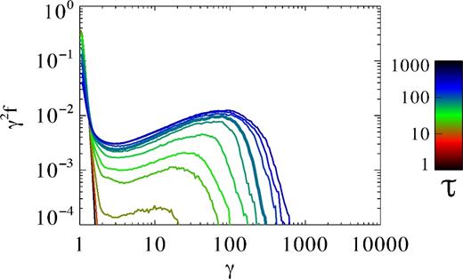
The evolution of the normalized particle energy spectrum γ2dN/dγ = γ2f with the normalized time τ = ct/(σrL) for Simulation S30. Successive spectra are approximately logarithmically spaced. The spectrum at the time of saturation τs ≈ 84 is shown using a thicker line. Note that our energy spectra here and in other plots do not include the contribution of the hot population of particles that began the simulation in the current sheet.
3.1.1 Saturation of the power law
To constrain the properties of this saturation more precisely, we fit the high-energy spectrum for simulations with all values of σ. Qualitatively, it is clear from Fig. 1 that a thermal spectrum is present at low energies that fully cuts off at approximately γ = 1.8. Then, an approximate power law begins at a location γi and ends with a possibly exponential cutoff at location γf.
This allows us to probe the properties of the power law and of the high-energy cutoff. The fitting of ζ allows us to compare our results with those of Werner et al. (2016), whose cutoff fitting function was the product of an exponential with ζ = 1 and one with ζ = 2. The value of γi where we begin fitting must be input to the fitting function, so we do fits for various values of this parameter and compare them. We select values for γi that are as small as possible without significantly worsening the fit.
Our fits show that saturation occurs at approximately the same time for all values of σ, which is at normalized saturation time τs ≈ 84. The only fitting parameter that does not saturate at this time is ζ, the shape of the high-energy cutoff. Table 1 shows the fitting parameters averaged over several inputs near this time of saturation, while Fig. 2 visually shows the particle energy spectra (solid lines) and the fits (dotted lines) to those spectra. The evolution of p with σ is generally consistent with that found by Werner et al. (2016) both qualitatively and quantitatively. p decreases monotonically with σ to an approximate asymptote at p ≈ 1.2, with p > 2 only for σ = 3. We also confirm their findings with respect to γf, which is indeed approximately 4σ for most values of σ. An exception to this is the case σ = 3, for which in any case we do not have enough dynamic range to obtain a good power-law fit.
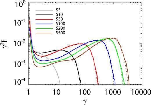
The normalized particle energy spectrum per logarithmic bin γ2dN/dγ = γ2f at the time of saturation τs ≈ 84 for each value of σ. The calculated fits above γi for each value of σ are shown using dashed lines.
Fits of simulations at saturation (τ ≈ 84).
| Runa | p | γi | γf | ζb | faccb,c | ⟨γ⟩accd | ⟨γ⟩ple | fintf |
|---|---|---|---|---|---|---|---|---|
| S3 | 2.23 | 1.8 | 6.4 | 1.5 | 0.42 | 3.1 | 3.1 | 0 |
| S10 | 1.72 | 2.4 | 34 | 2.3 | 0.74 | 7.4 | 8.2 | 0.037 |
| S30 | 1.46 | 2.9 | 132 | 2.4 | 0.89 | 18.4 | 20.4 | 0.026 |
| S100 | 1.24 | 10 | 434 | 2.1 | 0.91 | 80 | 88 | 0.053 |
| S200 | 1.19 | 19 | 847 | 2.1 | 0.92 | 167 | 179 | 0.071 |
| S500 | 1.16 | 36 | 2140 | 1.9 | 0.95 | 394 | 427 | 0.045 |
Notes.aThe number for each run gives the value of σ.
bThese parameters continue to evolve slowly after saturation.
cThe fraction of the particle kinetic energy in accelerated particles (those with Lorentz factor above γi).
dThe average Lorentz factor of accelerated particles.
eThe average Lorentz factor predicted for accelerated particles based on our power-law fits and equation (6).
fThe fraction of the particle kinetic energy in intermediate particles (those in the interval 1.8 < γ < γi).
The fraction facc of the particle energy in the power law at the saturation time τs ≈ 84 is also indicated in Table 1. The table indicates that the power-law particle population already has |$>\!90\,\,\rm{per\,\,cent}$| of the particle energy at saturation for σ > 10. Even for Simulation S3, facc > 0.7 at 2τs, which is a very short time on macroscopic scales. Thus, energy from the power-law population will dominate the radiation produced in reconnection, as generally assumed in models of this process.
Reconnection is an efficient process, as can be seen from the fact that the magnetization in the current sheet is of order unity [see fig. 3 of Kagan et al. (2016) for an example showing this]. We therefore expect that particles that experience full acceleration in the current sheet will receive an average energy of ⟨γ⟩ ≈ σ. Table 1 shows that ⟨γ⟩ ≥ 0.6σ in all cases.
We note that the commonly used approximation in which the γf term is dropped from the denominator and the γi term from the numerator is highly inaccurate for p < 2. Table 1 shows that the power law represents the overall energetics very well, within |$\pm 10\,\,\rm{per\,\,cent}$|, although it typically overestimates the average energy slightly.
We now discuss the uncertainties in our fits. The fit has a significant dependence on the choice of error model, but the resulting variation is not overwhelming so long as the fractional error in the distribution decreases as N(γ) increases. In the reported fits, we assume that errors in the spectrum are Gaussian in logarithmic space, proportional to |$1/\sqrt{\gamma N(\gamma )}$|. Uncertainties in the choice of error model and the choice of γi dwarf the calculated error for most of the parameters, imposing a significant uncertainty of at least ±0.1 in the power-law index p and of |$\pm 20\,\,\rm{per\,\,cent}$| in the location of the cutoff γi. The cutoff exponent ζ is very sensitive to the error model (but insensitive to γi), with approximate uncertainty ±0.2. The fitting uncertainties are significantly greater for the runs with σ = 3 and 500. In the earlier case, the shortness of the power-law portion of the spectrum makes it difficult to estimate the parameters of the fit, while in the latter case the shape of the spectrum appears to be less well described by our fitting function. These uncertainties and the trend in their magnitudes are roughly consistent with those found by Werner et al. (2016).
3.1.2 The lower limit of the power law and the intermediate population
The value of γi, the lower limit of the power law, is not reported by Werner et al. (2016). But it is crucial to understanding the particle energy spectrum produced in relativistic reconnection. This is well illustrated by Fig. 2, which compares the fits of particle spectra at saturation for all values of σ. While γi ≈ 2 for low σ, it increases significantly at larger values of σ, reaching an approximate value of σ/10 for Simulations S30, S100, and S200. The low value of γi = 36 ≈ 500/13.5 for Simulation 500 is not too surprising given the high uncertainty in the fit for this value of σ.
The fact that γi is far above the end of the thermal distribution at γ = 1.8 at high σ implies the presence of a significant population of particles in the interval 1.8 < γ < γi. These particles are neither unaccelerated like the background plasma nor fully accelerated to ⟨γ⟩ ∼ σ. We do not detect any significant difference between the locations in the current sheet of the intermediate particles and of the highest energy particles. This indicates that the intermediate particles go through the current sheet but receive little energy during the reconnection process.
The intermediate part of the spectrum as shown in Fig. 2 can be approximated as a power law with p ∼ 2, although the shape of the spectrum changes with σ. Thus, it is possible that at very high σ = 1000 the intermediate component of the spectrum expands or disappears. Table 1 shows that for σ > 3 these particles have fint ≈ 0.05 of the particle kinetic energy at the time of saturation. The variation in this number with σ is not systematic, and may result from uncertainties in the value of γi. fint does not change significantly following saturation, indicating that this part of the spectrum has also reached a steady state. We leave the investigation of the detailed properties of these intermediate particles to future work.
The values for γi shown in Table 1 imply that γf/γi ≈ 40 at large σ. This is a very narrow range and restricts the dynamic range of particle acceleration in reconnection. We discuss the implications of this result and the other properties of our fits for reconnection models of radiation from high-energy systems in Section 4.
3.1.3 Analysis of the high-energy cutoff
Fig. 3 shows how ζ depends on time for all values of σ except σ = 500. At the time of saturation, ζ ≈ 2.4 for Simulation S30 and ζ ≈ 2.1 for all other simulations with σ > 3. This is roughly consistent with the results of Werner et al. (2016), who found that at small system sizes the high-energy cutoff was well described with a cutoff corresponding to ζ = 2. After τs, ζ decreases monotonically with time. At τ = 2τs, ζ ≈ 1.3 for Simulations S100 and S200, ζ ≈ 1.6 for Simulation S10, and ζ ≈ 1.7 for Simulation S30.
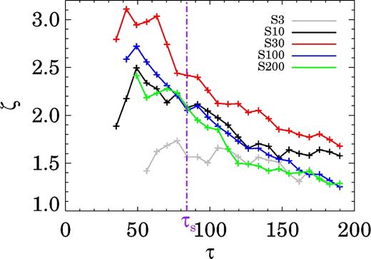
The evolution of ζ with normalized time τ for all values of σ except σ = 500, for which the simulation was not run for a long enough time to probe its evolution well beyond the saturation time of the other parameters. Data points are shown only for times at which a good fit to equation (5) could be found. The saturation time τs ≈ 84 is indicated using the dot–dashed line.
We have carried out some simulations at larger box size Lx = Ly = 500σrL to further investigate the evolution of ζ. They indicate that at late times the value of ζ continues to decrease, reaching approximately ζ ≈ 1.25 for σ = 30 and ζ ≈ 1.15 for σ = 100 at τ = 4τs. Comparing these results with the evolution in Fig. 3 indicates that the monotonic decrease in ζ slows at late times, but we do not see a clear asymptote in this evolution. Our results are roughly consistent with a cutoff at very late times that is asymptotically a simple exponential ζ = 1.0, as suggested by the results of Werner et al. (2016) for large reconnection systems. However, truly understanding the character of the high-energy cutoff will require future simulations with enough computer resources to probe the evolution of the particle energy spectrum over temporal and spatial scales larger than our simulations by an order of magnitude.
3.2 Analysis of particle acceleration
In order to find why the saturation of the power law at γf ≈ 4σ is occurring in our simulations (and those of Werner et al. 2016), we must first identify the primary acceleration process in the simulations. There are two methods for assigning significance to acceleration mechanisms. The first is an arithmetic measure, which compares the difference in Lorentz factor γafter − γbefore before and after each acceleration process. The second is a logarithmic measure, which instead compares the ratios γafter/γbefore for each process. The latter is the more important measure because acceleration can occur over several orders of magnitude and thus the logarithmically dominant process determines the shape of the spectrum.
To investigate the primary acceleration processes before and after saturation, we trace particles entering acceleration regions in the simulation with σ = 30 at ct/σrL ≈ 35 before saturation and at ct/σrL ≈ 140 after saturation. We initiate the particle tracing before and after saturation by duplicating particles flowing into X-points at these times and adding spread to their momenta and location. We then trace the particles for a period of τ ≈ 70 (105) for the pre-saturation (post-saturation) tracing.
Fig. 4 shows the structure of the simulation at these times, with the reconnection regions for which particle tracing is done highlighted with boxes and the initial locations of the traced particles entering the current sheet shaded in grey. From the figure, it is clear that the number of secondary islands in reconnection regions is increasing with time: there are no such islands in our chosen pre-saturation reconnection region, while there are between 2 and 9 islands of varying sizes in the post-saturation reconnection region (depending on the size needed for structures to be considered significant). Based on our more detailed study of current sheet structure(CSS) in Section 3.3, we find that there are three significant islands in this X-point that can deflect high-energy particles above γ = 4σ. The length of the primary reconnection regions has also increased approximately linearly with time, from D = 6.25σrL at ct/σrL ≈ 35 before saturation to D = 30σrL at ct/σrL ≈ 140 after saturation.
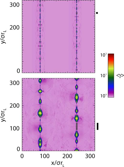
The current sheet structure throughout the simulation with σ = 30 displayed using the mean Lorentz factor ⟨γ⟩ at times τ ≈ 35 before saturation (top) and at τ ≈ 140 after saturation (bottom). The shaded boxes show the locations of the reconnection regions centred at (x0, y0) = (240, 263.3)σrL before saturation and (x0, y0) = (240, 110.75)σrL after saturation where we use test particles to probe the physics of particle accelerations. The edges of the boxes show the locations of particle injection, which are at x0 ± 3σrL with a spread of 2σrL. We repeat these boxes to the right of the figure for clarity.
Fig. 5 shows particle acceleration histories for two typical particles before and two other typical particles after saturation. It is clear from these figures that most of the energy gain for these particles occurs in a single, linear acceleration episode. For particles C (green) and D (blue) post-saturation and particle A (black) pre-saturation, it is clear that this acceleration takes place in the shaded X-point where the particle was injected. Even particle B (orange) in the pre-saturation run is accelerated in an X-point. The late time at which its acceleration begins is due to the fact that this X-point is not the one shaded in Fig. 4 but the one just above it.
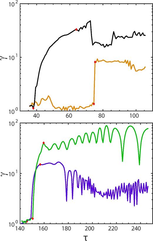
The particle acceleration history for two typical particles in the pre-saturation particle tracing beginning at τ ≈ 35 (top) and two other typical particles in the post-saturation particle tracing beginning at τ ≈ 140 (bottom) in Simulation S30. The particles are labelled with different colours as particles A (black), B (orange), C (green), and D (blue). The majority of the acceleration for all particles clearly occurs in a single rapid acceleration episode, consistent with X-point acceleration. This rapid acceleration phase is bounded with red diamonds.
We now consider the contribution of other acceleration mechanisms. Particle C (green) in the post-saturation run oscillates at late times as it reflects off of concentrations of Bx. This acceleration is clearly due to a Fermi process associated with either island contraction or curvature drift acceleration, as the acceleration per cycle increases with γ. However, this acceleration process increases the energy of the particle by a factor of only 2.
To confirm that these acceleration histories are indeed typical of the particle acceleration, we identify the rapid acceleration phase for each particle. This is done by selecting the period of monotonic increase in γ during which it increases by the greatest factor. Table 2 shows the averaged properties of the traced particles during the rapid acceleration phase for both the pre- and post-saturation tracing periods. We find that the particle energy at the end of this rapid acceleration phase is 13.7 (12.4) in the pre- (post-)saturation tracing. In both cases, this is more than 2/3 of the average energy ⟨γ⟩ = 18.4 of all accelerated particles throughout the simulation with σ = 30 shown in Table 1. This rapid acceleration also dominates the total acceleration experienced by the traced particles in the X-point, taking up more than 90 per cent (60 per cent) of the acceleration before (after) saturation. Furthermore, more than |$80\,\,\rm{per\,\,cent}$| of particles in both traces begin the rapid acceleration phase of acceleration at γ < 2, indicating that this phase is typically the first strong acceleration phase. This result favours X-point acceleration (independent of γ), over Fermi-type acceleration in which the energy gain is proportional to γ.
Properties of the rapid acceleration phase.
| τinja | ⟨γ⟩rb | ⟨γ⟩fc | f<2d | |$\langle E_{z}\rangle _{ \rm r}/B_0{}^{e}$| | ⟨vy⟩r/cf |
|---|---|---|---|---|---|
| 35 | 13.7 | 14.1 | 0.88 | 0,25 | 0.50 |
| 140 | 12.4 | 20.6 | 0.81 | 0.33 | 0.72 |
| τinja | ⟨γ⟩rb | ⟨γ⟩fc | f<2d | |$\langle E_{z}\rangle _{ \rm r}/B_0{}^{e}$| | ⟨vy⟩r/cf |
|---|---|---|---|---|---|
| 35 | 13.7 | 14.1 | 0.88 | 0,25 | 0.50 |
| 140 | 12.4 | 20.6 | 0.81 | 0.33 | 0.72 |
Notes.aThe approximate normalized time of injection.
bThe average Lorentz factor at the end of rapid acceleration.
cThe average Lorentz factor at the end of X-point acceleration.
dThe fraction of particles that begin rapid acceleration with γ < 2.
eThe average electric field in the z direction during the rapid acceleration phase, used in Section 3.3.
fThe average velocity in the y direction during the rapid acceleration phase, used in Section 3.3.
Logarithmically, X-point acceleration is even more dominant. X-point acceleration typically increases the particle energy by a factor of at least 12.4, while all other mechanisms combined produce at most an increase by a factor of ∼18.4/12.4 ≈ 1.48. Thus, X-point acceleration clearly determines the shape of the spectrum in our simulations.
Our results indicate that X-point acceleration by the reconnection electric field is indeed the dominant particle acceleration mechanism, in both the arithmetic and especially the logarithmic sense. Many studies find that alternative mechanisms are important arithmetically (Guo et al. 2014, 2015; Sironi & Spitkovsky 2014). But in the more important logarithmic sense, those studies usually1 still find that X-point acceleration is dominant (Sironi & Spitkovsky 2014; Guo et al. 2015). We note that this conclusion may change on extremely large scales not currently accessible to simulations, because acceleration during the many generations of island mergers that occur on such scales may become more energetically important than in current simulations.
3.3 Effects of CSS on the particle acceleration process
3.3.1 Conditions for the disruption of particle acceleration
Particle acceleration in the X-point therefore requires that the particle's momentum is (anti-)aligned with the electric field in the reconnection region, but a particle can be deflected when it encounters a magnetic island of sufficient size and magnetic field strength, disrupting the acceleration process. But since the deflection actually occurs at the edge of the island (or equivalently the adjacent X-point), we characterize both X-points and islands in a unified way, referring to them generically as CSS.
We approximately estimate that deflection by the strong magnetic field at the edge of an island (or equivalently X-point) will occur if the particle is strongly affected by the magnetic field Bc at the edge of a CSS before it can escape from the structure. The time required for escape is just Dc/⟨vy⟩, where Dc is the length of the CSS in the y direction and ⟨vy⟩ is the average velocity of the particle in the y direction as it crosses the structure. To estimate ⟨vy⟩, we calculate the average velocity ⟨vy⟩r/c for our test particles in Simulation S30 with σ = 30 during their rapid acceleration phases in X-points. We show in Table 2 that ⟨vy⟩r/c ≈ 0.50 on average before saturation and ⟨vy⟩r/c ≈ 0.72 afterwards, which is already quite large. Particles passing through a region of high magnetic field at the edge of a CSS will have an even larger velocity in that direction because the magnitude of vy increases monotonically during the rapid acceleration phase. Therefore, we set ⟨vy⟩ = c in this part of the analysis.
We schematically show in Fig. 6 how the deflection process works in the case of a magnetic island. The blue particle with γ ≫ γc is unaffected by the magnetic island and can undergo further acceleration in another X-point. In contrast, the red particle with γ ≪ γc is strongly deflected and then trapped in the island. As a result, it can no longer undergo significant acceleration. The comparison shows that particles only ‘see’ CSS with γc > γ. We show in Section 3.3.3 how this affects the saturation of particle acceleration.
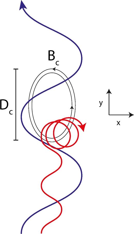
A schematic figure comparing the typical trajectories of a particle entering a magnetic island with γ ≪ γc (red) and with γ ≫ γc (blue). The red particle is quickly deflected by the strong magnetic field at the edge of the island (or equivalently the X-point) and is then trapped in the island. In contrast, the blue particle is basically unaffected by the magnetic field. The oscillations prior to entering the island are Speiser orbit trajectories characteristic of particle motion in X-points. Note that before entering the island, the largest component of the particles’ momentum is in the ±z direction (not shown) due to acceleration by the electric field.
3.3.2 Current sheet analysis
We can now investigate the structure of the current sheet to find Dc and Bc for each structure. We first find the maxima and minima of the reconnected field |Bx| over the length of the current sheet. Each of the minima corresponds to the centre of a CSS, while maxima correspond to the edges of a magnetic island or X-point. We hierarchically pair the maxima and minima in order to associate each location of large deflection with a CSS. For each pair, we can calculate Dc = 2(ymax − ymin) and Bc = (Bx, max − Bx, min)/2. The factor of 2 in the expression for Dc arises because the size of the structure is approximately the distance between two maxima (e.g. from one side of a magnetic island to another) or two minima (from an X-point to an island), not that between a maximum and a minimum. The factor of 1/2 in the expression for Bc arises because we estimate that the average magnetic field in the structure is around half of the maximum field. Finally, we can calculate γc using Dc, Bc, and equation (10).
Fig. 7 shows the locations ymin for highly significant CSS with γc > σ at the beginning of post-saturation particle tracing for Simulation S30. The minima calculated using our algorithm clearly correspond to minima of B0. These CSS typically be identified as X-points or magnetic islands from inspection or by reference to the simulation's density structure (as discussed in the figure caption). Note, however, that this identification has no effect on our results, which are based on generic properties of CSS.

The identification of CSS using our algorithm. The colours show the local magnetic field normalized to the background field B0 in Simulation S30 at the time τ ≈ 140 of post-saturation tracing. We focus on a region centred at the middle location of particle injection (x0, y0) = (240, 110.75)σrL at that time. The locations ymin of CSS are shown to the right of the main figure. The size of these symbols corresponds to which of two ranges of γc (shown to the right of the figure) the CSS corresponds to. X-points are labelled with an X and magnetic islands with a filled circle. They are differentiated by finding whether the structure corresponds to a maximum (island) or a minimum (X-point) in number density as well, although this identification is uncertain near the edges of the primary X-point at |y − y0| > 17σrL.
Fig. 8 shows Ns, the number of CSS with each value of γc in all of the simulations at the time of saturation τs ≈ 84. It is clear that the distribution of γc/σ does not depend significantly on σ for σ > 3. There are many small CSS with γc/σ ∼ 0.1, but the number of such structures quickly declines with increasing γc, levelling out at approximately γc = 4σ. Because increased particle acceleration no longer reduces the number of disruptive CSS encountered beyond this point, our result suggests that saturation of particle acceleration may occur near γ ≈ 4σ. We return to this argument in Section 3.3.3.
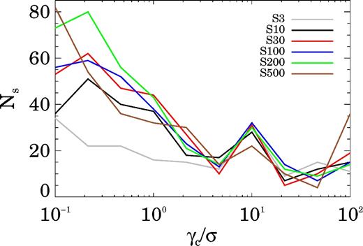
The number of CSS Ns at each value of γc/σ summed over three outputs near the time of saturation τs ≈ 84. We multiply the number of structures by 2 for Simulation S500, because the normalized system size in that simulation was half of that found in the other simulations. It is clear that the distribution does not depend strongly on σ for σ > 3.
3.3.3 CSS and the saturation of particle acceleration
This would give the correct final Lorentz factor if particles were accelerated in only one structure. But particles do not finish their acceleration unless they encounter a CSS with γc > γ. Thus, the size of the acceleration region actually encountered by a particle depends on the particle energy. The typical size of acceleration regions for particles with γ ∼ γc can be estimated as ⟨D⟩(γc), defined as the median distance between CSS with structure parameter larger than γc. We normalize this quantity to σrL in our calculations, as we do with all length-scales in this paper.
Fig. 9 shows how this parameter varies with γc. It is clear that the distance between CSS increases slowly and monotonically with γc approximately as |$\gamma _{\rm c}^{1/3}$| at low γc, levelling off somewhat at higher γc. ⟨D⟩/σrL is basically independent of σ for σ > 3, just as Ns is. We note that 10σrL is the approximate size of CSS predicted by Werner et al. (2016) based on a heuristic argument using the results of Larrabee, Lovelace & Romanova (2003) and Kirk & Skjæraasen (2003). Here, we confirm that this result is approximately correct for γc ≈ 4σ and somewhat low for γc > 10σ.
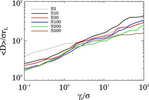
The median distance ⟨D⟩/σrL between CSS with parameter larger than γc for all simulations. This distance is clearly independent of σ. For low γc, this distance grows as |$\gamma _{\rm c}^{1/3}$|, but it levels out at higher γc.
Because ⟨D⟩/σrL is independent of σ as seen in Fig. 9, this equation indicates that γmax ∝ σ. Thus, the spontaneous formation of CSS with a separation proportional to σrL provides a physical explanation for the saturation of the power law in our fits.
While equation (14) is still implicit, it is clear that there are two regimes for γmax depending on the ratio γmax/γc. If γmax > γc, particle acceleration in X-points with parameter of at least γc tends to result in the particle reaching high enough energy to be unaffected by a significant number of large CSS. This makes further acceleration more probable. In contrast, if γmax < γc, particles will not accelerate enough to reduce their susceptibility to deflection by CSS. As a result, we expect that such particles will not accelerate beyond γmax. This will produce a cutoff at γmax = γc.
In Fig. 10, we plot the ratio γmax/γc as a function of γc. The figure shows that γmax/γc decreases monotonically with γc approximately as |$\gamma _{\rm c}^{-2/3}$|. Fig. 10 shows that γmax = γc at around γc ≈ 5σ, which is close to the location of the cutoff that we find in fits of the power-law particle energy spectrum.
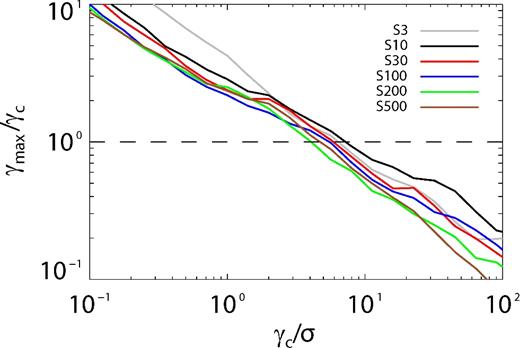
The ratio γmax/γc as a function of γc. When the ratio falls below 1 (shown with the dashed line), particle acceleration above γ is no longer possible due to the intervention of significant CSS.
Fig. 9 shows that the value of γmax = ⟨D⟩/2σrL is typically around 30σ for γc = 100σ. Because particles accelerating in large X-points with γc ≫ 4σ cannot reach higher Lorentz factors than γmax, we expect almost no particles to reach above γ = 30σ, which is less than a factor of 10 higher than the cutoff. This indicates that the cutoff should be sharp, consistent with an exponential or super-exponential. Thus, our current sheet analysis has correctly predicted the existence and the location at γ ≈ 4–5σ of a sharp high-energy cutoff of the power law in the particle energy spectrum produced in relativistic reconnection.
It has commonly been thought that because current sheet evolution produces larger and larger primary X-points and magnetic islands, the properties of the particle energy spectrum in reconnection are determined by global dynamics. But we have shown that spontaneous tearing in large X-points continually produces magnetic islands with a characteristic size of ∼σrL, which implies that the maximum γ ∼ σ. Our detailed analysis gives a more precise cutoff at γ ≈ 4σ. Thus, the small-scale properties of the current sheet can never be ignored in investigating reconnection even though the global dynamics dominate the overall structure. Constraints from this small-scale structure have significant effects on reconnection models of astrophysical emission, as we show in the next section.
4 APPLICATION TO ASTROPHYSICAL SOURCES
We now discuss the implications of our results in Section 3.1 for the application of relativistic reconnection to observed radiation from high-energy astrophysical sources. We note that these conclusions may be unreliable if new acceleration mechanisms become important in very large scale systems. In addition, the application of our results to ion–electron plasmas still needs to be confirmed. In this section, we assume that our conclusions scale to very large scales found in astrophysical systems and that our pair plasma results apply to any ion–electron plasmas that may be present in such systems.
We have shown in Section 3.1.1 that the power-law index found in reconnection falls in the range 1.15 < p < 2.3. The power-law index of synchrotron radiation resulting from particles in the power law is typically either −p/2 (if cooling is fast) or −(p − 1)/2 (if cooling is slow; Sari et al. 1998). This corresponds to a range of flux per logarithmic interval νFν ∝ ν−0.15–ν0.9. Thus, reconnection produces nearly flat or rising logarithmic radiation spectra. In Section 3.1.2, we have shown that the extent of the power law in the particle energy spectrum is quite narrow: γf/γi ≤ 40. The corresponding maximum dynamic range of the high-energy synchrotron spectrum emitted by the particles is ≈402 = 1600.
This narrow range can be expanded if significant relativistic bulk flows or variations in the magnetic field are present because the energy at the synchrotron peak is proportional to BΓ. Ultrarelativistic bulk flows with Γ ≫ 1 are rarely produced in relativistic reconnection (Guo et al. 2014; Melzani et al. 2014; Kagan et al. 2016), although they may occur for some initial conditions (Sironi et al. 2016). The variation in B in the outskirts of magnetic islands where particles emit is also relatively small, typically no more than a factor of a few (as can be seen in Fig. 7). Overall, we estimate that BΓ does not vary by more than a factor of 5 for particles in a given reconnection region. Variability in the central source or resulting from global instabilities may also be a source of variation in BΓ. If we roughly estimate that the variation in BΓ from these sources is similar to the variation in the location of the spectral peak, we can estimate the size of this effect for any given source.
We now consider whether these properties of reconnection are consistent with various observed astrophysical systems. We first consider the flares in the Crab's PWN (Abdo et al. 2011; Striani et al. 2011; Tavani et al. 2011; Buehler et al. 2012; Mayer et al. 2013), which extend for around 1.5 decades in frequency below the peak of the distribution, with a sharp cutoff above it. It is possible that the power law extends a bit further at low energies where it is swamped by the quiescent spectrum, but this dynamic range is still easily consistent with reconnection. The flare spectra near the peak frequency are nearly flat in νFν at the peak time of the flares. Therefore, the reconnection model with a relatively low σ works well for the Crab flares.
The TeV flares in AGN (Aharonian et al. 2007, 2009; Albert et al. 2007; Tavecchio et al. 2013; Cologna et al. 2017) have a power-law spectrum with some curvature that extends for around 2 decades in frequency. This range can easily be produced by reconnection. The intrinsic power-law spectra of Fermi-Large Area Telescope (LAT) blazars have hard power-law indices in the range νFν ∝ ν−0.65–ν−0.15 (Singal, Petrosian & Ajello 2012). Flaring galaxies have quiescent spectra consistent with these values, but the flaring spectra are typically harder (Albert et al. 2008; Abramowski et al. 2012; Cologna et al. 2017). Thus, most TeV flares are consistent with being produced in reconnection at low σ, or even at moderate σ in extraordinary cases.
Finally, we consider the prompt phase of GRBs. In many GRBs in the Fermi catalogue, the combined Gamma-ray Burst Monitor (GBM) and LAT data are consistent with a single power-law component over a large frequency range. In GRB 0901003, the prompt emission observed by Fermi appears to constitute a single power law from a peak at ∼400 keV in the GBM instrument all the way up to ∼2.8 GeV as observed in the LAT instrument (Zhang et al. 2011). The peak of the energy spectrum varied by a factor of only 1.5 during the burst, so variation in BΓ likely cannot expand the power-law range of reconnection (which is less than 1600) enough to explain the observed dynamic range of 7000 for the GRB. While this GRB is an extreme case, many other GRBs observed in the LAT band have a directly observed dynamic range of around 1000–3000 in frequency with no strong evidence of a cutoff beyond that range (Ackermann et al. 2013). It not easy to explain such GRBs in a reconnection model.
Additional evidence against the direct application of reconnection to prompt GRB emission comes from spectral slopes. Fits to the high-energy portion of the spectrum of GRB range from νFν ∝ ν−2.8–ν−0.6 (Gruber et al. 2014), significantly softer than in reconnection even at low σ. Thus, it seems difficult for relativistic reconnection to produce the non-thermal emission seen in the prompt phase of GRBs. In summary, it appears that relativistic reconnection is clearly applicable to the Crab flares and to TeV flares in AGN, and has difficulty accounting for the prompt GRB emission.
5 CONCLUSIONS
In this paper, we investigated the saturation of the high-energy power-law spectrum in reconnection using PIC simulations at various magnetizations σ. We used particle tracing to identify the dominant particle acceleration mechanism as direct acceleration by the reconnection electric field in X-points. We then analysed the structure of the current sheets in our simulations to show that the spontaneous formation of secondary islands and X-points (referred to as CSS) was responsible for saturation.
Our conclusions are as follows.
The high-energy part of the particle energy spectrum produced by reconnection can be fitted with a hard power law followed by a super-exponential cutoff.
The high-energy power law in the particle energy spectrum saturates at γf ≈ 4σ. This saturation occurs at the normalized time τ ≈ 84, consistent with the saturation at L = 40σrL found by Werner et al. (2016).
The ratio γf/γi, where γi is the minimum energy of the power law, approaches ≈40 at large σ.
Our particle tracing reveals that X-points are responsible for the majority of particle acceleration, especially in a logarithmic sense. The average energy of particles after a single episode of rapid acceleration in the X-point is at least |$70\,\,\rm{per\,\,cent}$| of the average energy of all accelerated particles after saturation.
We find that the saturation of particle acceleration in reconnection is due to the spontaneous production of magnetic islands within large X-points. At the edges of the magnetic islands, strong magnetic fields are present that can deflect particles and end particle acceleration. We characterize CSS including both X-points and magnetic islands in a unified way by the maximum Lorentz factor γc of particles that the adjacent strong magnetic fields can deflect.
The distribution of γc/σ is largely independent of σ. It declines quickly at small γc but plateaus at γc ≈ 4σ. This is consistent with saturation of the power law at γf ≈ 4σ.
We calculate an implicit equation for the maximum acceleration possible in CSS as a function of their typical size and γc parameter. We find that particles entering the current sheet can be accelerated to a maximum energy of approximately 5σ before they are deflected by an encounter with a significant CSS and their acceleration is stopped. This is very close to the location of the high-energy cutoff we find in our fits.
Our results indicate that the fundamental spatial scale for particle acceleration is of the order of σrL. Because secondary islands and X-points are constantly produced at this scale, it remains important even at late times when primary islands and X-points are much larger than σrL.
Our simulations predict that particles accelerated in reconnection will produce synchrotron spectra that are hard power laws with index νFν ≈ ν0 and a narrow frequency range of ∼1600. TeV AGN flare spectra and Crab PWN flare spectra, which are hard and have narrow frequency ranges, can easily be produced by reconnection. In contrast, the relatively soft and broad power laws present in prompt GRB emission are difficult to produce in reconnection.
ACKNOWLEDGEMENTS
This research was supported by the I-CORE Center for Excellence in Research in Astrophysics and by an ISA grant. DK and TP were partially supported by a CNSF-ISF grant. EN was partially supported by an ISF grant and by an ERC starting grant. DK was also supported by the GIF (grant I-1362-303.7/2016) and by the ISF within the ISF-UGC joint research program (grant No. 504/14).
Footnotes
In the study of Guo et al. (2014), it is unclear whether X-point acceleration or a first-order Fermi process involving curvature drift is logarithmically dominant because some details of the acceleration process are not shown. But later work from the same researchers (Guo et al. 2015) confirms that X-point acceleration is logarithmically dominant in their simulations.
REFERENCES
