


Abstract
We use integral field spectroscopic (IFS) observations from Gemini Multi-Object Spectrograph North (GMOS-N) of a group of four H ii regions and the surrounding gas in the central region of the blue compact dwarf (BCD) galaxy NGC 4670. At spatial scales of ∼9 pc, we map the spatial distribution of a variety of physical properties of the ionized gas: internal dust attenuation, kinematics, stellar age, star formation rate, emission-line ratios, and chemical abundances. The region of study is found to be photoionized. Using the robust direct Te method, we estimate metallicity, nitrogen-to-oxygen ratio, and helium abundance of the four H ii regions. The same parameters are also mapped for the entire region using the HII-CHI-mistry code. We find that log(N/O) is increased in the region where the Wolf–Rayet bump is detected. The region coincides with the continuum region, around which we detect a slight increase in He abundance. We estimate the number of WC4, WN2-4, and WN7-9 stars from the integrated spectrum of WR bump region. We study the relation between log(N/O) and 12 + log(O/H) using the spatially resolved data of the field of view as well as the integrated data of the H ii regions from 10 BCDs. We find an unexpected negative trend between N/O and metallicity. Several scenarios are explored to explain this trend, including nitrogen enrichment, and variations in star formation efficiency via chemical evolution models.
1 INTRODUCTION
Chemical evolution of the Universe is one of the most explored topics in astrophysical research and is essential to unravel the secrets of cosmic origin. All chemical elements result from nucleosynthetic processes, which happened either after a few seconds of the Big Bang or in the first stars after the Dark Ages and then during the subsequent evolutionary stages of stars and are still happening today in the present-day galaxies. Consequently, this topic has been the subject of innumerable observational and theoretical studies, as we continue to investigate various aspects of chemical evolution (see e.g. Pagel 1997; Izotov & Thuan 1998; Matteucci 2003; Tremonti et al. 2004; Erb et al. 2006; Maiolino et al. 2008; Steigman 2007; Mannucci et al. 2010; Davé, Finlator & Oppenheimer 2012; Mollá et al. 2015).
The study of the relation between nitrogen-to-oxygen ratio and oxygen abundance has been a topical subject of investigation and debate in both observing (e.g. McCall, Rybski & Shields 1985; Thuan, Izotov & Lipovetsky 1995; Izotov et al. 2006; Amorín, Pérez-Montero & Vílchez 2010; Berg et al. 2012; James et al. 2015; Belfiore et al. 2017) and modelling (e.g. Edmunds 1990; Henry, Edmunds & Köppen 2000; Köppen & Hensler 2005; Mollá et al. 2006; Vincenzo et al. 2016) communities working on chemical evolution. Nitrogen is of special interest as its origin is both primary and secondary. It may be produced from stars whose gas mixture contains only H and He (primary origin), and also from stars whose initial gas mixture contain metals (secondary origin). Thus, the production of nitrogen may or may not depend on the initial metallicity of the gas. The relative abundance of nitrogen and oxygen is regulated by various factors such as star formation history, presence of low- and high-mass stars, local chemical pollution possibly due to supernovae or Wolf–Rayet (WR) stars, and the flow of gas in, out, and within the galaxies (Edmunds 1990; Henry et al. 2000; Köppen & Hensler 2005; Mollá et al. 2006; Vincenzo et al. 2016). Hence, mapping the distribution of physical properties of the ionized gas within galaxies is essential in understanding not only the nucleosynthetic origin of nitrogen but also the chemical enrichment and recycling processes.
Chemical abundances of galaxies can be robustly estimated and mapped by using the direct Te method, which requires the detection of weak auroral lines (e.g. [O iii] λ 4363, [N ii] λ 5755). In the absence of such detections, indirect methods are used for estimating the chemical abundances, which involve the use of strong emission lines. These indirect methods may be either the well-established calibrations involving the emission-line ratios (e.g. Pettini & Pagel 2004; Maiolino et al. 2008; Pérez-Montero & Contini 2009; Dopita et al. 2016; Curti et al. 2017), or using the emission-line fluxes in the photoionization models of the ionized nebulae, such as cloudy (Ferland et al. 2013) and mappings (Sutherland & Dopita 1993). Some examples of the codes that use such models to calculate abundances are hii-chi-mistry (Pérez-Montero 2014), izi (Blanc et al. 2015), and bond (Vale Asari et al. 2016).
Blue compact dwarf galaxies (BCDs; Searle & Sargent 1972; Thuan & Martin 1981) in the local Universe are ideal laboratories for mapping chemical abundance, as they host luminous H ii regions that emit in the visible range, hence providing a plethora of the emission lines required for chemical abundance analysis. Moreover, BCDs are low-metallicity (1/50–1/3 Z⊙), starbursting dwarf galaxies in the nearby Universe, whose properties [e.g. metallicity, compactness, specific star formation rate (SFR), and gas fraction] resemble those which are observed in primeval galaxies at high redshift (see Kunth & Östlin 2000, for a review). Their proximity enables detailed in-depth analyses of a variety of physical properties for both the young (Hunter & Thronson 1995; Papaderos et al. 1998; Thuan, Izotov & Foltz 1999) and more evolved stellar components (Papaderos et al. 1996; Gil de Paz, Madore & Pevunova 2003; Cairós et al. 2007; Amorín et al. 2009). However, most of these analyses are based on either long-slit and/or photometric observations (e.g. Izotov & Thuan 1999; Cairós et al. 2001a,b; Hägele et al. 2012), which do not allow us to simultaneously map the chemical abundances and other physical properties within the BCDs. As such, any information on the spatial correlation between different physical properties and chemical abundance patterns are lost.
With the advent of integral field spectroscopy (IFS), the study of BCDs have been revolutionized (e.g. James et al. 2009; James, Tsamis & Barlow 2010; James et al. 2013a,b; Lagos et al. 2012, 2014, 2016; Westmoquette et al. 2013) as IFS has enabled to spatially resolve the distribution of the physical properties of the ISM within the BCDs. This has allowed statistical analysis of these distributions to explore the spatial uniformity or homogeneity of such properties within BCDs (Pérez-Montero et al. 2011, 2013; Kehrig et al. 2013, 2016). IFS also allows us to analyse the spatial correlation between different properties; for example, using IFS, Kehrig et al. (2008) detected both a WR population and an excess N/O across the BCD IIZw70; López-Sánchez et al. (2011) detected WR features and He ii λ4686 emission line at the same location in the BCD Ic10, and Kumari, James & Irwin (2017) reported signatures of shock ionization in the spatially resolved emission-line ratio diagrams and the velocity structure of the ionized gas of the central H ii region of the BCD NGC 4449. Hence, IFS studies are essential in understanding the cause and effect of various physical processes taking place in the ISM of the BCDs.
This paper is the second in a series of IFS analyses of star-forming regions in BCDs (see Kumari et al. 2017), where we aim to gain a deeper insight into the physical properties of these systems, by answering the following related questions: (1) How are the nitrogen-to-oxygen ratio (N/O) and oxygen abundance (O/H) distributed in the region of study? (2) Which physical mechanism is primarily responsible for the ionization of gas? (3) What is the age of the stellar population currently ionizing the gas in the target region of study? In this paper, we have targeted the central region of NGC 4670 (Fig. 1), a BCD (Gil de Paz et al. 2003) that has appeared in many studies comprising large sample of star-forming galaxies (e.g. Hunter, Gallagher & Rautenkranz 1982; Hunter 1982; Kinney et al. 1993; Moustakas & Kennicutt 2006; Brauher, Dale & Helou 2008; Haynes et al. 2011; James et al. 2014).
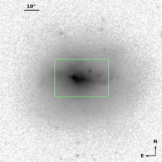
SDSS r-band image, showing the bright central region and an elliptical halo of older stellar population in NGC 4670. The green rectangular box shows region covered by the HST image shown in Fig. 2.
NGC 4670 is an ideal target for addressing these questions and specifically for studying the relation between N/O and O/H. Besides being classified as a BCD, it has also been recognized as a WR galaxy (Mas-Hesse & Kunth 1999). As such, we expect local chemical pollution resulting from the winds of the WR stars, which may lead to chemical enrichment of the ISM and an enhanced N/O. Being a BCD, it is expected to have a low-metallicity and high SFR. In fact, neutral hydrogen observations of NGC 4670 show a high concentration of the gas in the centre of the galaxy (Hunter et al. 1996), which may also increase the star formation. A multiwavelength analysis of the galaxy by Huchra et al. (1983) indicates the presence of several hundred O stars in giant H ii region complexes, which indicate that the galaxy hosts young stellar populations. It is therefore possible that the metallicity, star formation, or stellar properties might be spatially correlated with the WR stellar population or N/O. Moreover, this galaxy is relatively close (∼18.6 Mpc), as such the high spatial sampling (0.1 arcsec) provided by the integral field unit (IFU) on the Gemini Multi-Object Spectrograph North (GMOS-N) has allowed us to study the spatial correlation between these properties at a spatial scale of 9 pc. A previous IFS study of the entire galaxy was performed using Visible Integral Field Replicable Unit Spectrograph (VIRUS-P), but had a spatial sampling of 4.2|${\rm \,arcsec}$| or 350 pc Cairós et al. (2012). Our study presents for the first time the IFS observation of NGC 4670, at a very fine spatial sampling of 0.1|${\rm \,arcsec}$| hence allowing a detailed analysis of spatial properties. Moreover the IFS data has enabled us to identify four new luminous H ii regions in this galaxy. General properties of NGC 4670 are given in Table 1.
General properties of NGC 4670.
| Parameter | NGC 4670 |
|---|---|
| Other designation | UGC 07930, Haro 9, Arp 163 |
| Galaxy Type | BCD, WR |
| RA (J2000.0) | 12h45m17|${^{\rm s}_{.}}$|1 |
| Dec. (J2000.0) | +27d07m31s |
| Redshift (z)a | 0.003 566 ± 0.000 013 |
| Distance (Mpc)a | 18.6 |
| Inclination (°)b | 28 |
| Helio radial velocity (km s−1)a | 1069 ± 4 |
| E(B − V)c | 0.0128 ± 0.0003 |
| M|$_B^b$| | −18.6 |
| (U − B)b | −0.49 |
| 12 + log(O/H)d | 8.30 |
| M* (M⊙)e | 10|$^{8.78^{+0.2}_{-0.17}}$| |
The paper is organized as follows. Section 2 presents the observation and data reduction. Section 3 presents the preliminary procedures required for further data analysis and the main results, which include the gas kinematics, chemical abundances, and stellar properties. In Section 4, we explore the relation between the nitrogen-to-oxygen ratio and oxygen abundance at the spatially resolved scale, and for the H ii regions in this BCD. We also do a comparative analysis with a sample of H ii regions within nine more BCDs compiled from the literature, a sample of green peas and also a large sample of star-forming galaxies from the Sloan Digital Sky Survey (SDSS). We explore the observed trend in the relation with the chemical evolution models. We finally summarize our results in Section 5.
2 OBSERVATION and DATA REDUCTION
The target region of NGC 4670 was observed with the GMOS (Hook et al. 2004) and IFU (GMOS-N IFU; Allington-Smith et al. 2002) at Gemini-North telescope in Hawaii, in one-slit queue-mode. This observation mode provides a field of view (FOV) of 3.5|${\rm \,arcsec}$| × 5|${\rm \,arcsec}$| sampled by 750 hexagonal lenslets of projected diameter of 0.2 arcsec, of which 250 lenslets are dedicated to sky background determination. Table 2 presents information from the data observing log. Observations were carried out in four different settings using grating B600+_G5307 (B600) and grating R600+_G5304 (R600), covering the blue and red regions of the optical spectrum, respectively. To avoid the problems in wavelength coverage due to two chip gaps between the three detectors of GMOS-N IFU, two sets of observations were taken with spectral dithering of 50 Å. For each of the four settings, a set of standard observations of GCAL flats, CuAr lamp for wavelength calibration, and standard star for flux calibration were taken.
GMOS-N IFU observing log for NGC 4670.
| Grating | Central wavelength | Wavelength range | Exposure time | Average airmass | Standard star |
|---|---|---|---|---|---|
| (Å) | (Å) | (s) | |||
| B600+_G5307 | 4650 | 3196–6067 | 2 × 1550 | 1.16, 1.24 | Hz44 |
| B600+_G5307 | 4700 | 3250–6118 | 3 × 1550 | 1.015, 1.034, 1.066 | Wolf1346 |
| R600+_G5304 | 6900 | 5345–8261 | 2 × 1400 | 1.013, 1.008 | Wolf1346 |
| R600+_G5304 | 6950 | 5397–8314 | 2 × 1400 | 1.12, 1.038 | Wolf1346 |
The basic steps of data reduction including bias subtraction, flat-field correction, wavelength calibration, sky subtraction, and differential atmospheric correction, were carried out using the standard GEMINI reduction pipeline written in Image Reduction and Analysis Facility (iraf).1 However, the standard pipeline does not provide satisfactory results for some procedures and we therefore had to develop and implement our own codes. For example, wavelength calibration of the observations in one of the red settings and the flux calibration of the observations in one of the blue settings did not agree with the observations in the other three settings. We corrected the offset in wavelength calibration by comparing with the redshift obtained from the blue setting. Similarly, we statistically determined the scaling factor in the flux of the spectra in the blue setting. More information about these and other corrections procedures can be found in Kumari et al. (2017). We used the routine gfcube available in Gemini's iraf reduction package to convert the spectra in each setting into three-dimensional data cubes, where we chose a spatial sampling of 0.1|${\rm \,arcsec}$| that was adequate to preserve the hexagonal sampling of GMOS-IFU lenslets. We corrected the spatial offset and spectral dithering between the observations of the same grating while combining the cubes obtained from that grating. The FOV covered by the two gratings (B600 and R600) showed a spatial offset of 0.1|${\rm \,arcsec}$| and 0.2 arcsec in the x- and y-axes (with Fig. 2 as reference). We produced cubes and row-stacked spectra of the overlapping regions of the FOVs covered by the two gratings, which we used for further analysis. For both red and blue settings, we fitted a Gaussian profile to several emission lines of the extracted row-stacked spectra of the arc lamp and found the value of instrumental broadening (full width at half-maximum, FWHM) to be ∼1.7 Å.
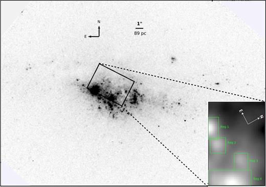
Left-hand panel: HST image of NGC 4670 taken in the filter F439W. The black rectangular box in the centre represents the GMOS aperture (3.5|${\rm \,arcsec}$| × 5|${\rm \,arcsec}$|). The HST image has a spatial scale of 0.05 arcsec pixel−1. North and east on the image is shown by the compass on the top left of the figure. Right-panel panel: H α map of the FOV obtained from the GMOS-IFU shows the four H ii regions (Reg 1, Reg 2, Reg 3, Reg 4) in green rectangular boxes. The compass on this panel shows north and east on our FOV.
3 RESULTS
3.1 Observed and intrinsic fluxes
3.1.1 Flux measurement
Fig. 2 (left-hand panel) shows the Hubble Space Telescope (HST) image of NGC 4670 taken in the filter F435W. The black rectangular box represents the GMOS aperture (3.5 arcsec × 5 arcsec). The lower right-hand panel presents the distribution of H α emission line (obtained from GMOS) across the FOV, and clearly shows four regions (green rectangular boxes labelled as ‘Reg 1’, ‘Reg 2’, ‘Reg 3’, and ‘Reg 4’) of current/increased star formation activity. These regions have been selected by visually inspecting the H α emission-line map and roughly identifying isophotal regions. The present analysis includes the spatially resolved and integrated properties of these four H ii regions, which are referred to as regions 1, 2, 3, and 4 in the following. Note here that all analysis related to regions 1 and 4 should be treated with more caution since the GMOS-FOV does not cover these regions completely. In Fig. 3, we show the GMOS-IFU integrated spectra of these four regions in the blue and red parts of the optical spectrum. The principal emission lines are overplotted at their rest wavelengths in air.
![GMOS-IFU integrated spectra of individual H ii regions in the FOV in the blue (upper panel) and red (lower panel) settings. The spectra of the four H$\,\small {II}$ regions are colour-coded as follows: region 1: blue, region 2: green, region 3: red, region 4: orange. The blue ends of the spectra are noisier due to the low sensitivity of GMOS-IFU, which makes it difficult to show [O ii] λλ3727, 3729 line in log scale. We show the [O ii] λλ3727, 3729 line for all regions in Fig. 4, along with the spectral line fitting.](https://oup.silverchair-cdn.com/oup/backfile/Content_public/Journal/mnras/476/3/10.1093_mnras_sty402/1/m_sty402fig3.jpeg?Expires=1750096609&Signature=a6Ndh3f6eyY0CL5VAVTP~QkEF7neDVx21xJAJiHe0FysJvyXkOATlWlGnCfvtnLU31CzSIOSnT2D2~Rlh90SDyIpb-5OY0mk6HKlzCu0tUiTZgr8ghFfjF783TKDLxtJbWbFB8wmdoamQvm-ps-rEtLxd0FUHqMlfqVcD-Q8pPRLh9V8Qqn6Y8yR2y0KemR1CLiISXgQd4h6AurPWI~VkO-YzXPRdmjaocy77kKjfOhgUMDYx4oV~HJJJL13Ap9LUCpgIbZJhnBtYZEjnWIYUY1TNgTG-sb~bfWwHQBpxT-rzyU6X9-eS~JdqBfwkUuVNOFIcu5K23XnsH14dvjyhw__&Key-Pair-Id=APKAIE5G5CRDK6RD3PGA)
GMOS-IFU integrated spectra of individual H ii regions in the FOV in the blue (upper panel) and red (lower panel) settings. The spectra of the four H|$\,\small {II}$| regions are colour-coded as follows: region 1: blue, region 2: green, region 3: red, region 4: orange. The blue ends of the spectra are noisier due to the low sensitivity of GMOS-IFU, which makes it difficult to show [O ii] λλ3727, 3729 line in log scale. We show the [O ii] λλ3727, 3729 line for all regions in Fig. 4, along with the spectral line fitting.
We measure the emission-line fluxes for all the main recombination and collisionally excited lines within the spectra by fitting Gaussian profiles to emission lines after subtracting the continuum and absorption features in recombination lines in the spectral region of interest. A single Gaussian profile was used to fit each emission line. Fig. 4 shows the Gaussian fits for the [O ii] doublet, where the peaks of the two emission lines [O ii] λλ3727, 3729 could be hardly resolved for the four star-forming regions. In the spaxels where the peaks of the two emission lines in the [O ii] doublet could not be resolved at all, we fitted a single Gaussian. While fitting Gaussian to the emission lines, we gave equal weight to flux in each spectral pixel since the dispersion in the continuum flux is found to be constant in the spectral region of interest both in the calibrated and uncalibrated spectra. This shows that the uncertainty of flux determination within a spectral window is constant. Our error estimates on fluxes are the errors obtained while fitting Gaussians to the emission lines. The uncertainty related to the level of continuum is very small, hence the error on the flux is dominated by the error on the Gaussian fitting. The error estimates are consistent with those estimated from a Monte Carlo simulation. The fitting errors have been propagated to the other quantities using Monte Carlo simulations in subsequent analysis.
![In the four panels corresponding to four H ii regions, the upper panel shows the continuum-subtracted [O ii] λλ3727, 3729 line (blue curve) detected in each region along with the ‘Gaussian’ fit (red curve) to extract flux, and the lower panels show the residuals normalized to be in σ-noise units.](https://oup.silverchair-cdn.com/oup/backfile/Content_public/Journal/mnras/476/3/10.1093_mnras_sty402/1/m_sty402fig4.jpeg?Expires=1750096609&Signature=2dPpoAguf2Hsn~h~tbtvjj~d26WkZ~mRwhZE~xsNfBcRdZDm9n3HIWi77Kt4n0eOaF69AHVIN1hCCaFwoMJ2UofOoofqOC3iaqegM-G5BTPDVDBgEcm0HSCBsp19Z0QUB~4zHrgvw-roa1LqPmP8bu1hKEUEpToBxrygGMSP9e15CeE-oI7Kxy57lApcnPcIbgd~Rjb99YtMBEfJosdo5auWREvWoncoBGamWYD-2ZN9OUrocRAdBb6GrlD36fQOeA4FYQwzz16ZDeJOoKKpeAG6IBZfMPE1q3ANGMTIGIEsAmKO10z1eCxSFLr7~OZTDKHuo-QH742gtcaU5-fcxA__&Key-Pair-Id=APKAIE5G5CRDK6RD3PGA)
In the four panels corresponding to four H ii regions, the upper panel shows the continuum-subtracted [O ii] λλ3727, 3729 line (blue curve) detected in each region along with the ‘Gaussian’ fit (red curve) to extract flux, and the lower panels show the residuals normalized to be in σ-noise units.
Fig. 5 shows the observed flux maps of the GMOS FOV of B-band continuum, [O ii] λλ3727, 3729, [O ii] λ5007, H α, [N ii] λ6584, and [S|${\small II}$|] λ6717. White spaxels in all maps correspond to the spaxels in which emission lines have S/N < 3. The B-band continuum map is obtained by integrating the blue cube in the wavelength range of 3980–4920 Å (in the rest frame). The spatial profile of the continuum map remains same irrespective of the masking of emission lines. Table 3 presents the observed fluxes for the main emission lines used in the present analysis obtained from the integrated spectra of the four H ii regions (Fig. 3; ‘Reg 1’, ‘Reg 2’, ‘Reg 3’, and ‘Reg 4’ shown in Fig. 2).
![Observed B-band continuum map and the emission-line flux maps ([O ii] λλ3727, 3729, [O ii] λ5007, H α, [N ii] λ6584, and [S${\small II}$] λ6717) of NGC 4670. The four black rectangular boxes denote the location of the four H ii regions. White spaxels correspond to the spaxels in which emission-line fluxes had S/N < 3.](https://oup.silverchair-cdn.com/oup/backfile/Content_public/Journal/mnras/476/3/10.1093_mnras_sty402/1/m_sty402fig5.jpeg?Expires=1750096609&Signature=pWdHuZsxyXtaTmhqxzv1FhjWmvpjhRQXhw2RwJgvobbg59gUBd-ixjd~uibKBn1ATVK8lfc0NLF5JW2O3aGJgRymREm1PxTGBMTA6RlMypllakW1eHAxi-anPx~WfZ2ldMhrxGKN8bum77UYPXQXNF1VkiniHWjFXuMR8B8~NZzLo1LWg0o2Q~piYFzULMMJiQquj8~RPipFIoshEhZHVXd5R2J8XInXd389d2RM6NjrRAmDTsQTOrwloPehCd9N5oCOTiwiMKCwC0WxE8QpdaRUG~ByMR4q3RvMZGVUkln2JBzIrZxdxy4Y4de-pX7u8Ctci1zQskOSjql~y7pBjA__&Key-Pair-Id=APKAIE5G5CRDK6RD3PGA)
Observed B-band continuum map and the emission-line flux maps ([O ii] λλ3727, 3729, [O ii] λ5007, H α, [N ii] λ6584, and [S|${\small II}$|] λ6717) of NGC 4670. The four black rectangular boxes denote the location of the four H ii regions. White spaxels correspond to the spaxels in which emission-line fluxes had S/N < 3.
Emission-line measurements (relative to H β = 100) for the integrated spectra of the four H ii regions shown in Fig. 2. Line fluxes (Fλ) are extinction corrected using E(B − V) to calculate Iλ for each of the individual H ii regions.
| Line | λair | F1λ | I1λ | F2λ | I2λ | F3λ | I3λ | F4λ | I4λ |
|---|---|---|---|---|---|---|---|---|---|
| |$[{\rm O\,\small {II}}]$| | 3726.03 | 127.88 ± 3.63 | 135.57 ± 6.02 | 147.14 ± 4.43 | 154.48 ± 7.10 | 178.38 ± 6.28 | 197.62 ± 8.68 | 153.60 ± 3.22 | 169.56 ± 5.85 |
| |${\rm H\,}\gamma$| | 4340.47 | 44.82 ± 0.80 | 45.97 ± 1.66 | 43.88 ± 0.56 | 44.82 ± 1.54 | 43.08 ± 0.52 | 45.03 ± 1.22 | 42.76 ± 0.35 | 44.63 ± 1.18 |
| |$[{\rm O\,\small {III}}]$| | 4363.21 | 2.78 ± 0.35 | 2.84 ± 0.37 | 1.84 ± 0.24 | 1.88 ± 0.25 | 1.64 ± 0.24 | 1.72 ± 0.26 | 1.26 ± 0.15 | 1.31 ± 0.16 |
| Hβ | 4861.33 | 100.00 ± 0.58 | 100.00 ± 2.15 | 100.00 ± 0.56 | 100.00 ± 2.18 | 100.00 ± 0.41 | 100.00 ± 1.65 | 100.00 ± 0.42 | 100.00 ± 1.71 |
| |$[{\rm O\,\small {III}}]$| | 4958.92 | 141.05 ± 1.00 | 140.47 ± 4.19 | 99.58 ± 0.71 | 99.24 ± 3.02 | 81.17 ± 0.46 | 80.59 ± 1.86 | 91.76 ± 0.51 | 91.13 ± 2.18 |
| |$[{\rm O\,\small {III}}]$| | 5006.84 | 418.30 ± 3.02 | 415.64 ± 12.33 | 294.67 ± 2.24 | 293.11 ± 8.89 | 242.41 ± 1.53 | 239.72 ± 5.53 | 273.50 ± 1.71 | 270.57 ± 6.48 |
| |${\rm He\,}{\rm \small {I}}$| | 5875.67 | 12.28 ± 0.24 | 11.81 ± 0.39 | 12.95 ± 0.18 | 12.54 ± 0.38 | 13.18 ± 0.14 | 12.31 ± 0.28 | 12.66 ± 0.14 | 11.85 ± 0.29 |
| |$[{\rm N\,\small {II}}]$| | 6548.03 | 4.88 ± 0.47 | 4.60 ± 0.46 | 7.09 ± 0.58 | 6.75 ± 0.58 | 9.66 ± 0.49 | 8.72 ± 0.47 | 7.80 ± 0.54 | 7.07 ± 0.51 |
| |${\rm H\,}\alpha$| | 6562.8 | 303.46 ± 1.97 | 286.00 ± 7.42 | 300.48 ± 1.99 | 286.00 ± 7.57 | 317.31 ± 1.59 | 286.00 ± 5.72 | 316.16 ± 1.65 | 286.00 ± 5.96 |
| |$[{\rm N\,\small {II}}]$| | 6583.41 | 15.30 ± 0.48 | 14.41 ± 0.58 | 22.40 ± 0.60 | 21.31 ± 0.79 | 30.07 ± 0.51 | 27.08 ± 0.69 | 24.11 ± 0.55 | 21.79 ± 0.66 |
| |$[{\rm S\,\small {II}}]$| | 6716.47 | 13.96 ± 0.16 | 13.10 ± 0.36 | 19.92 ± 0.21 | 18.90 ± 0.52 | 28.14 ± 0.22 | 25.18 ± 0.52 | 20.99 ± 0.18 | 18.86 ± 0.41 |
| |$[{\rm S\,\small {II}}]$| | 6730.85 | 10.37 ± 0.15 | 9.73 ± 0.28 | 14.73 ± 0.19 | 13.96 ± 0.40 | 20.39 ± 0.20 | 18.24 ± 0.39 | 15.24 ± 0.17 | 13.68 ± 0.31 |
| |$[{\rm O\,\small {II}}]$| | 7318.92 | 1.80 ± 0.06 | 1.67 ± 0.07 | 2.09 ± 0.07 | 1.95 ± 0.08 | 2.28 ± 0.11 | 1.99 ± 0.10 | 2.09 ± 0.11 | 1.84 ± 0.10 |
| |$[{\rm O\,\small {II}}]$| | 7329.66 | 1.34 ± 0.05 | 1.24 ± 0.06 | 1.70 ± 0.06 | 1.59 ± 0.07 | 1.87 ± 0.10 | 1.63 ± 0.09 | 1.64 ± 0.09 | 1.44 ± 0.08 |
| E(B − V) | 0.057 ± 0.006 | 0.048 ± 0.006 | 0.099 ± 0.005 | 0.096 ± 0.005 | |||||
| F(H β) | 28.46 ± 0.17 | 34.37 ± 0.74 | 25.20 ± 0.14 | 29.50 ± 0.64 | 19.31 ± 0.08 | 26.90 ± 0.44 | 87.11 ± 0.36 | 119.92 ± 2.06 |
Notes. F(H β) in units of × 10−15 erg cm−2 s−1.
3.1.2 Dust attenuation
where k(λH β) and k(λH α) are the values from the Large Magellanic Cloud (LMC) attenuation curve (Fitzpatrick 1999)2 evaluated at the wavelengths H β and H α, respectively, |$({\rm H}\,\alpha /{\rm H\,}\beta )_{{\rm obs}}$| and |$({\rm H}\,\alpha /{\rm H\,}\beta )_{{\rm theo}}$| denote the observed and theoretical |${\rm H}\,\alpha /{\rm H\,}\beta$| line ratios, respectively. We chose the LMC attenuation curve because the metallicity of NGC 4670 is reported to be 12 + log(O/H) = 8.30 (Hirashita et al. 2002), which is close to that of LMC, 8.35 ± 0.06 (Russell & Dopita 1992).
Following the above procedure, we found negative values of E(B − V) for some spaxels in random regions of the FOV, which we forced to the ‘Galactic foreground’ E(B − V) value (= 0.0128). The negative values of E(B − V) could be due to dominance of shot noise in the low-extinction regions (Hong et al. 2013; Kumari et al. 2017). Fig. 6 shows the map of E(B − V), which varies from 0.012 to 0.60 mag across the FOV. We find that the four H ii regions have relatively lesser dust attenuation than the rest of the regions in the FOV. The E(B − V) map appears to be similar to the continuum map (Fig. 5, upper right-hand panel), i.e. the region to north-west of the group of H ii regions with weak continuum is more extincted. To investigate this further, we compared the continuum maps of NGC 4670 in the B and R bands, our colour (B − R) map resembles the E(B − V) map. The Balmer decrements |$({\rm H}\,\alpha /{\rm H\,}\beta )$| observed for the four H ii regions are in agreement with the results of Huchra et al. (1983), who report it to be approximately 3 from the broad-band photometric data of NGC 4670. Our results are consistent with works of Huchra et al. (1983), whose optical data indicate little internal extinction.
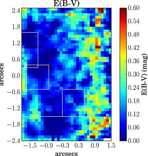
E(B − V) map created assuming the LMC extinction curve. Spaxels with E(B − V) < 0 are set to E(B − V) of the Galactic foreground. The four white rectangular boxes denote the location of the four H ii regions. White spaxels correspond to the spaxels in which emission-line fluxes had S/N < 3.
3.2 Gas kinematics
Fig. 7 shows the maps of radial velocity and velocity dispersion (FWHM) of the H α emission line, obtained from the centroid and width of the Gaussian fit to the emission line. We correct the radial velocity map for the barycentric correction (= −13.74 km s−1) and systemic velocity of 1069 km s−1 of NGC 4670 (Wolfinger et al. 2013). We also correct the FWHM maps for the instrumental broadening of 1.7 Å of GMOS-IFU.
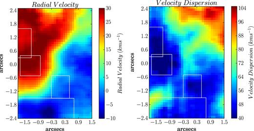
Radial velocity (left) and FWHM (right) maps of the ionized gas obtained from the H α emission line. Radial velocity is corrected for systemic (= 1069 km s−1) and barycentric velocities (= −13.74 km s−1). FWHM is corrected for instrumental broadening (= 1.7 Å). The four white rectangular boxes denote the location of the four H ii regions.
The radial velocity map (Fig. 7, left-hand panel) shows that the ionized gas is slowly rotating about an axis of rotation going diagonally (NE-SW) through the FOV. The radial velocity varies between ∼ −10 and 30 km s−1. The gas is redshifted in H ii regions 1 and 2, while it is blueshifted in regions 3 and 4. Our velocity map shows a isovelocity S-shaped contour, which is in agreement with the [O iii] velocity map of the entire galaxy presented by Cairós et al. (2012). Note here that their one spatial element covers our entire FOV.
The FWHM map (Fig. 7, right-hand panel) shows a variation of 40–104 km s−1 across the FOV. 3 All the H H |$\small {II}$|regions have a relatively lower velocity dispersion compared to the rest of the FOV.
3.3 Emission-line ratio diagnostics
Fig. 8 shows the classical emission-line ratio diagnostic diagrams ([O iii] λ5007/H β versus [S ii] λλ6717, 6731/H α, right-hand panel, and [O iii] λ5007/H β versus [N ii] λ6584/H α, left-hand panel), commonly known as BPT diagrams (Baldwin, Phillips & Terlevich 1981), which present a powerful tool to identify the ionization mechanisms at play in the ionized gas. On both diagnostic diagrams, the solid black line represents the maximum starburst line, known as the ‘Kewley line’ (Kewley et al. 2001), showing classification based on excitation mechanisms. The emission-line ratios lying below and to the left of the Kewley line can be explained by the photoionization by massive stars, while some other source of ionization [e.g. active galactic nuclei (AGNs) or mechanical shocks] is required to explain the emission-line ratios lying above the Kewley line. On the [N ii] λ6584/H α diagnostic diagram (Fig. 8, right-hand panel), the dashed black curve indicates the empirical line derived by Kauffmann et al. (2003) based on the SDSS spectra of 55 757 galaxies. The zone enclosed between this empirical curve and the theoretical ‘Kewley line’ is referred to as the composite zone. The emission-line ratios corresponding to the four H ii regions (see Table 4) derived from their integrated spectra are shown as blue circle (region 1), green pentagon (region 2), red square (region 3), and orange diamond (region 4). The spatially resolved (spaxel-by-spaxel) emission-line ratios in the FOV for different regions are shown, using the same colour and markers but smaller sizes. In addition, we also show the line ratios in the spaxels that are not covered by any of the four star-forming regions by magenta coloured markers. We find that both the integrated and spatially resolved data lie below and to the left of the Kewley line. Evidently no data lies in the composite region, hence confirming photoionization by massive stars as the dominant ionization mechanism in the target region of NGC 4670. Note here that the composite zone may also be assigned to pure H ii regions with very high N/O (Pérez-Montero & Contini 2009). Although we see some local N pollution in and around some H ii regions in our sample (Fig. 11), this is not enough to make our regions lie in the composite zone. Previous IFS studies of resolved H ii regions in BCDs have shown that low-excitation spaxels can lie in the AGN region [see e.g. Pérez-Montero et al. (2011) and Kumari et al. (2017) for BCDs HS0128+2832, HS 0837+4717, and NGC 4449, respectively]. However, this is not the case for the spatially resolved data in the BCD under study (NGC 4670).
![Emission-line ratio diagnostic diagrams: [O iii]/H β versus [S ii]/H α (left), and [O iii]/H β versus [N ii]/H α (right). Black solid curve and dashed curve represent the theoretical maximum starburst line from Kewley et al. (2001) and Kauffmann et al. (2003), respectively, showing a classification based on excitation mechanisms. The line ratios of the four H${\small II}$ regions are colour coded as follows: region 1: blue circle, region 2: green pentagon, region 3: red square, region 4: orange diamond. Smaller markers denote the spatially resolved (spaxel-by-spaxel) line ratios and the bigger markers denote the line ratios obtained from the integrated spectrum of the corresponding regions. Magenta-coloured markers denote the spatially resolved line ratios of the regions of FOV excluding the four H ii regions. The size of error bars varies for line ratios and the median error bars are shown in the right corner of each panel. The error bars on the line ratios obtained from the integrated spectra of the four H ii regions are smaller than the markers used here.](https://oup.silverchair-cdn.com/oup/backfile/Content_public/Journal/mnras/476/3/10.1093_mnras_sty402/1/m_sty402fig8.jpeg?Expires=1750096609&Signature=o0qfw9SI4I~yk0YT-dXe62Bm4z61T5ibxg0ffmlqvAA4rKs1mg5kiVPMZzAqtO7bvc6DV0N~GOfIZq5Lt8ALXJEWLwKBQiQ~tj6cSHi3-E9i9dFUFP5txwB9dTUGoiclsCgTVLjqjWZwaIHrW1cieAe4ICOd2ODxP2igPIXAkhZgKXqc4MXCO35lavTFYRHej1Ly2tt93EUBrQVmJY1mrrGGyHgEJECXq1n8MDEVq0S68~ODO3~CUapFMgFuUvLYa7MhoquT6T1VcEjMgkWyg3hpk00BxcxrHFwh0S-l7D8Ubga0ONkuLC4I1YfpWxCZw9cQNOoKOmqIYshVbUBG7A__&Key-Pair-Id=APKAIE5G5CRDK6RD3PGA)
Emission-line ratio diagnostic diagrams: [O iii]/H β versus [S ii]/H α (left), and [O iii]/H β versus [N ii]/H α (right). Black solid curve and dashed curve represent the theoretical maximum starburst line from Kewley et al. (2001) and Kauffmann et al. (2003), respectively, showing a classification based on excitation mechanisms. The line ratios of the four H|${\small II}$| regions are colour coded as follows: region 1: blue circle, region 2: green pentagon, region 3: red square, region 4: orange diamond. Smaller markers denote the spatially resolved (spaxel-by-spaxel) line ratios and the bigger markers denote the line ratios obtained from the integrated spectrum of the corresponding regions. Magenta-coloured markers denote the spatially resolved line ratios of the regions of FOV excluding the four H ii regions. The size of error bars varies for line ratios and the median error bars are shown in the right corner of each panel. The error bars on the line ratios obtained from the integrated spectra of the four H ii regions are smaller than the markers used here.
Integrated properties of the four H ii regions of NGC 4670 in the GMOS-FOV.
| Ionization Conditions | ||||
|---|---|---|---|---|
| Region 1 | Region 2 | Region 3 | Region 4 | |
| log (|$[{\rm O\,\small {III}}]\, \lambda 5007 / {\rm H}\,\beta$|) | 0.621 ± 0.003 | 0.469 ± 0.003 | 0.385 ± 0.003 | 0.437 ± 0.003 |
| log (|$[{\rm N\,} {\rm \small {II}}]\, \lambda 6583 /{\rm H}\,\alpha$|) | −1.297 ± 0.013 | −1.128 ± 0.011 | −1.023 ± 0.007 | −1.118 ± 0.01 |
| log (|$[{\rm S\,\small {II}}]\, \lambda \lambda 6717,6731/{\rm H}\,\alpha$|) | −1.096 ± 0.004 | −0.938 ± 0.003 | −0.815 ± 0.003 | −0.941 ± 0.003 |
| Abundance Analysis | ||||
| Region 1 | Region 2 | Region 3 | Region 4 | |
| Te(O iii) (K) | 10100 ± 400 | 9900 ± 400 | 10200 ± 500 | 9200 ± 300 |
| Te(O ii) (K) | 10500 ± 400 | 11000 ± 400 | 9700 ± 300 | 10000 ± 200 |
| Ne (cm−3) | 80 ± 30 | 70 ± 30 | <50 | <50 |
| 12 + log(O+/H+) | 7.58 ± 0.06 | 7.55 ± 0.07 | 7.89 ± 0.06 | 7.77 ± 0.05 |
| 12 + log(O++/H+) | 8.17 ± 0.06 | 8.05 ± 0.06 | 7.91 ± 0.07 | 8.12 ± 0.05 |
| 12 + log (O/H) | 8.27 ± 0.05 | 8.17 ± 0.05 | 8.21 ± 0.05 | 8.28 ± 0.04 |
| log(N/O) | −1.16 ± 0.07 | −1.02 ± 0.08 | −1.11 ± 0.07 | −1.11 ± 0.06 |
| y+ (He i 5876) | 0.088 ± 0.003 | 0.093 ± 0.003 | 0.092 ± 0.002 | 0.086 ± 0.002 |
| Stellar Properties | ||||
| Region 1 | Region 2 | Region 3 | Region 4 | |
| EW(H α) (Å) | ∼97 | ∼152 | ∼334 | ∼265 |
| Age (sub-Z⊙) (Myr) | ∼24 | ∼22 | ∼16 | ∼17 |
| SFR (Z⊙)(× 10−3M⊙yr−1) | 20.3 ± 0.3 | 17.5 ± 0.3 | 15.9 ± 0.2 | 70.9 ± 0.8 |
| SFR (sub-Z⊙)(× 10−3M⊙yr−1) | 13.4 ± 0.2 | 10.8 ± 0.2 | 10.1 ± 0.1 | 47.1 ± 0.6 |
We can study the spatial structure of the ionization through the relevant line ratio maps shown in Fig. 9. The H ii regions, particularly regions 1, 2, and 4, show low values of [N ii] λ6584/H α (upper left-hand panel) and [S ii] λλ6717, 6731/H α (upper right-hand panel), and high values of [O ii] λ5007/H β (lower panel), indicating that the corresponding regions have relatively high excitation. This is likely due to the presence of a harder ionizing field from hot-massive stars in the respective H ii regions. These regions are also brighter in the B-band continuum (Fig. 5, upper left-hand panel), supporting our inference of the presence of massive stars.
![Emission-line ratio maps of $[{\rm N}\,{\rm \small {II}}]\, \lambda 6583 /{\rm H}\,\alpha$, $[{\rm S} {\rm \,\small {II}}]\, \lambda \lambda 6717, 6731/{\rm H\,}\alpha$ and $[{\rm O\,\small {III}}]\, \lambda 5007 /{\rm H}\,\beta$. The four black rectangular boxes denote the location of the four H ii regions. White spaxels correspond to those spaxels with emission-line fluxes having S/N < 3.](https://oup.silverchair-cdn.com/oup/backfile/Content_public/Journal/mnras/476/3/10.1093_mnras_sty402/1/m_sty402fig9.jpeg?Expires=1750096609&Signature=1QSx0IohG2wlgbusgMiVCu3mjEN5TuVyS2JlS9ZV-4z1-obfQ1Qcz0btgfUEO6zlX3vewo1h4Kp7dr0bxwAjmvl3uXqryoXX4KaCFaVDA4W33OItsDx10zTC~jp5RXh03X5qIxzJ2wNFgCQeMIZfZY2LlqLYeNoV6p4wYnsuSnpRn0SvarJBje3XrGyX79BWd9nTZW85cCr8rdT8xLLzUnvm3JWQHDl~GgR5PsyWl74quPToCL1zoXkESl8YbYRlennbrby~eo3HSF5RrwEmlwXC8es4LiiHIvTO67-B3edONFtrgDdfbU9oDg-cvH-nR~t7-~RZq8K7LjIJKxs1EA__&Key-Pair-Id=APKAIE5G5CRDK6RD3PGA)
Emission-line ratio maps of |$[{\rm N}\,{\rm \small {II}}]\, \lambda 6583 /{\rm H}\,\alpha$|, |$[{\rm S} {\rm \,\small {II}}]\, \lambda \lambda 6717, 6731/{\rm H\,}\alpha$| and |$[{\rm O\,\small {III}}]\, \lambda 5007 /{\rm H}\,\beta$|. The four black rectangular boxes denote the location of the four H ii regions. White spaxels correspond to those spaxels with emission-line fluxes having S/N < 3.
3.4 Chemical abundances
3.4.1 Integrated spectra chemical abundances
We estimate chemical abundances of the four H ii regions in the target region of NGC 4670 from their integrated spectra (Fig. 3) by the direct method (i.e. using electron temperatures and collisionally excited lines). All emission-line fluxes are reddening-corrected for chemical abundance determination. Table 4 summarizes the chemical properties of the four H ii regions.
Electron temperature and density: The first step in estimating chemical abundance by the direct method is the determination of electron temperature(Te) and density (Ne). We derive Te ([O iii]) from the dereddened [O iii] line ratio, [O iii] (λ5007 +λ4959)/[O iii] λ4363, and the expression from Pérez-Montero (2017), which is obtained assuming a five-level atom, using collision strengths from Aggarwal & Keenan (1999), and is valid in the range of 7000–25 000 K. The estimated Te ([O iii]) for the four H ii regions vary from ∼9200 to 10 200 K (Table 4).
Using the derived Te ([O iii]) value for each star-forming region and the corresponding [S ii] doublet ratio λ6717/λ6731 from the integrated spectra, we compute Ne ([S ii]) of the four H ii regions (Table 4). We find Ne to be low in all the four H ii regions, with values < 50 cm−3 in regions 3 and 4. Such low densities and derived Te ([O iii]) are common within H ii regions (Osterbrock & Ferland 2006).
To derive the temperature of the low-ionization zone Te ([O ii]), we employ the expression given in Pérez-Montero (2017),4 which uses the ratio of oxygen doublets ([O ii] (λ3726 + λ3729)/[O ii] (λ7319 + λ7330)), in combination with the electron density Ne (derived above). The expression is valid in the range of 8000–25 000 K, where the collision coefficients are taken from Pradhan et al. (2006) and Tayal (2007). The estimated Te ([O ii]) of the four H ii regions vary from ∼9700 to 11 000 K (Table 4).
Oxygen abundance: Oxygen is used as a proxy for total metallicity because it is the most prominent heavy element observed in the optical spectrum in the form of O0, O+, O2 +, and O3 +. We employ the formulations of Pérez-Montero (2017) to calculate O+/H+ and O2 +/H+ using Te ([O ii]) and Te ([O iii]), respectively, i.e. the electron temperatures of the ionization zone dominated by the corresponding ions. The O+/H+ and O2 +/H+ are combined to calculate the elemental O/H for all four H ii regions given in Table 4. The values of 12 + log(O/H) vary between 8.17 and 8.28, with a mean = 8.23 and standard deviation = 0.04. These values fall in the transition region between the intermediate- and the high-metallicity regime that we discuss further in Section 4.
Previous studies reported the metallicity of NGC 4670 using only indirect methods. For example, Mas-Hesse & Kunth (1999) estimates 12 + log(O/H) = 8.4 from a 11 arcsec slit spectrum, while Cairós et al. (2012), calculated metallicity using another strong-line calibration, the P-method (Pilyugin & Thuan 2005) and reported 12 + log(O)/H = 8.29 for the entire galaxy (∼80 arcsec × 80 arcsec) and 12 + log(O/H) = 8.37 for the nuclear region (|${\sim }40{\rm \,arcsec}$| × 40|${\rm \,arcsec}$|). The mean metallicity of 12 + log(O/H) = 8.23 calculated from the direct method in this work is lower than all those values, which is consistent with the systematic offsets existing between different metallicity diagnostics as noted by Kewley & Ellison (2008). Moreover, the region under study in this work is much smaller (∼3.5 arcsec × 5 arcsec) than the previous studies.
Nitrogen-to-oxygen ratio: Assuming the low-ionization zone temperature Te ([O ii]) and density Ne ([S ii]) derived above, we use the emission-line ratio of ([N ii](λ6584 + λ6584)/H β formulation from Pérez-Montero (2017) to derive log(N+/H+) for all four H ii regions. Assuming that N+/O+ = N/O, we use log(N+/H+) and log(O+/H+) to derive log(N/O). These values agree with those derived directly from ([N ii]λ6584/ [O ii] (λ3726 + λ3729)) using the log(N/O) formula from Pérez-Montero (2017).4 The log(N/O) values of the four H ii regions vary between −1.02 and −1.16, with a mean of −1.10 and a standard deviation of 0.05.
Helium abundance: We use the reddening-corrected He i 5876 line in combination with Te ([O ii]) and Ne ([S ii]) derived above to calculate the helium abundances (y+) of the four H ii regions. Other helium lines are not used as they are either weak (S/N < 3) or affected by absorption of underlying stellar populations in one or more H ii regions. The expression for theoretical emissivities are taken from Pérez-Montero (2017), and the optical depth function is assumed to be one. This assumption on optical depth along with the contamination of He lines due to underlying absorption feature would result in an uncertainty of only ∼2 per cent in the helium abundance (Hägele et al. 2008). The y+ values for the four H ii regions vary between 0.086 and 0.093, with a mean of 0.090 and standard deviation of 0.003.
3.4.2 Spatially resolved chemical abundances
To map chemical abundance using the robust Te method, we require the detection of a weak auroral line throughout the FOV. Unfortunately, the S/N ratio of [O iii]λ4363 in the individual spectrum across the FOV was too low (<3) to use the direct Te method. Various indirect methods involving the use of strong emission lines have been devised to estimate chemical abundances to overcome this problem. Some of the popular indirect methods involve the use of the N2 parameter (Denicoló, Terlevich & Terlevich 2002), O3N2 parameter (Pettini & Pagel 2004), R23 (Pagel et al. 1979), N2S2H α (Dopita et al. 2016), or a combination of them (e.g. Maiolino et al. 2008; Curti et al. 2017). We used three of these strong line methods in our analysis of another BCD, NGC 4449 (Kumari et al. 2017), and found the well-known problem of the offsets between the metallicities from the direct and indirect method (Kewley & Ellison 2008). In this work, instead, we make use of the publicly available python-based code hii-chi-mistry (v3.0)5. This code takes the dereddened fluxes, follows a χ2-based methodology on a grid of photoionization models, including cloudy and popstar, and outputs chemical abundances (O/H, N/O) (Pérez-Montero 2014). The errors on the output abundances are calculated by the code using a Monte Carlo iteration from the reported errors of the measured lines. By using this code, we aim to remove the dependence of oxygen abundance on the nitrogen-to-oxygen ratio, which is an inherent assumption in some of the strong line calibrators. This becomes useful when we study the spatially resolved (O/H) versus (N/O) later in Section 4.
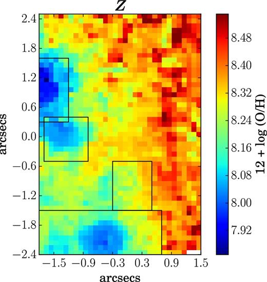
Oxygen abundance: Fig. 10 shows the metallicity map of the FOV obtained from the hii-chi-mistry code. The value of 12 + log(O/H) varies between ∼7.80 and 8.56 with a mean value of = 8.29 and standard deviation = 0.13. We find that region 1 is metal-poor compared to the other three H ii regions. However, metallicity estimates obtained from the integrated spectra of the four H ii regions show that regions 1 and 4 have comparable metallicities. This is likely due to an aperture effect, i.e. when we integrate over the large regions, the temperature and metallicity gets dominated by the brightest regions and becomes luminosity weighted. Thus even though region four hosts a range of metallicities, it is dominated by the large low-metallicity blob that has similar metallicity to that of region 1 as inferred from the integrated spectra. The mean value of spatially resolved log(O/H) agrees with the mean value calculated from the integrated spectra of the four H |$\small {II}$|regions within ±1 standard deviation.
Metallicity map obtained using the H II-CHI-mistry code. The four black rectangular boxes denote the location of the four H ii regions. White spaxels correspond to the spaxels in which emission-line fluxes had S/N < 3.
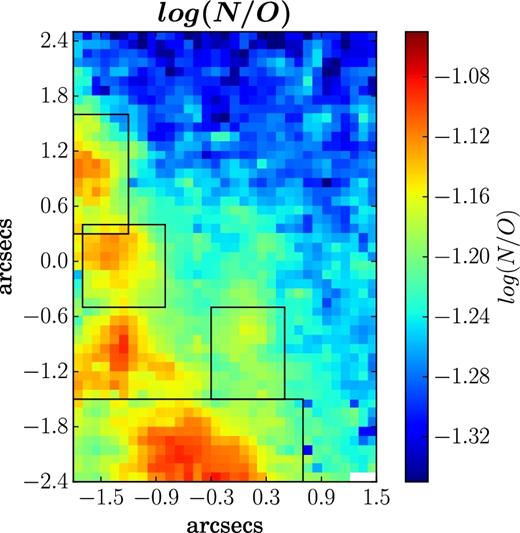
Nitrogen-to-oxygen ratio: Fig. 11 shows the log(N/O) map of the FOV from the hii-chi-mistry code. The value of log(N/O) varies between −1.4 and −1.08, with a mean value of = −1.23 and standard deviation = 0.06. We find that there is an increase in log(N/O) values in the region surrounded by the three H ii regions 2–4. This is probably a region which formed stars in the past but is quiescent now, resulting in a relatively chemical-enriched ionized gas. The log(N/O) map also shows that region 3 has a relatively lower log(N/O) value compared to other H ii regions; however, it is the integrated spectrum of region 1 that shows the highest log(N/O) (Table 4). This is likely due to aperture effects as explained above. The mean value of spatially resolved log(N/O) agrees with the mean value calculated from the integrated spectra of the four H ii regions within ±2 standard deviations.
log(N/O) map obtained using the hii-chi-mistry code. The four black rectangular boxes denote the location of the four H ii regions. White spaxels correspond to the spaxels in which emission-line fluxes had S/N < 3.
The maps of log(O/H) and log(N/O) show signatures of chemical inhomogeneity though the significance is low because of high error bars. We explore the homogeneity of chemical abundances in an upcoming paper (Kumari et al., in preparation).
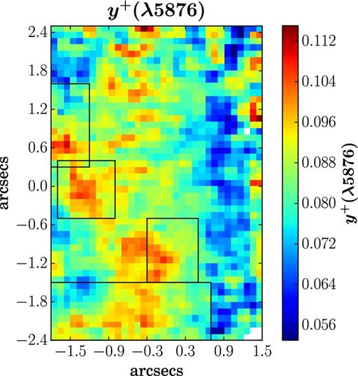
Helium abundance: For mapping helium abundance (y+), we require spatially resolved electron temperature and density measurements. As mentioned earlier, such maps could not be made because of the low S/N of the weak auroral line [O iii] λ4363. So we create the Te ([O iii]) map by using the hii-chi-mistry derived metallicity map (Fig. 10), and the relation between log(O/H) and Te ([O iii]) from Pérez-Montero (2017) (proposed initially in Amorín et al. 2015). We use the Te ([O iii]) map in conjunction with spatially resolved [S ii] doublets to map Ne across the FOV.6 Amongst all the He lines detected in our data (He i 4471, 5876, 6678, and 7065 Å, He ii 4686), the flux map corresponding to He i λ5876 has the highest S/N across the entire FOV. Hence, we use the dereddened flux map of He i λ5876 along with the Te ([O iii]) and Ne maps to create the helium abundance map (Fig. 12). The theoretical emissivities and the optical depth function are same as described in Section 3.4.1. Comparing the helium abundance map (Fig. 12) with the B-band continuum (Fig. 5), we find that there is a relative increase of y+ in the regions surrounding the continuum. Given that the continuum indicates the region with a relatively older population, it is likely that the winds emanating from the outer atmosphere of these stars or cluster of stars have resulted in an increase in y+ in the surrounding regions.
Helium abundance map obtained from He i λ5876 flux map. The four black rectangular boxes denote the location of the four H ii regions. White spaxels correspond to the spaxels in which emission-line fluxes had S/N < 3.
3.5 Stellar properties
3.5.1 Age of stellar population
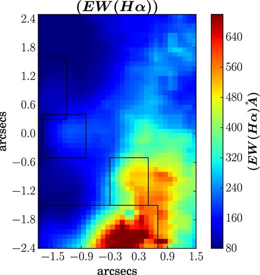
The integrated spectra of the four H ii regions (Fig. 3) show Balmer emission lines indicating the presence of young, hot, and massive O and B stars, and Balmer absorption lines (H β, H γ, etc.) indicating the presence of early-type A stars. For age-dating the current ionizing population, we first map the equivalent width (EW) of H α recombination line as shown in Fig. 13. The EW values show a variation of 48–776 Å across the FOV. Such high values of EW(H α) have been found in H ii regions in the local BCDs (e.g. I Zw 18, Mrk 475, Mrk 1236, NGC 2363 by Buckalew, Kobulnicky & Dufour 2005). Considering higher redshifts, Shim et al. (2011) found EW(H α) = 140–1700 Å for a galaxy sample in the redshift range of 3.8 < z < 5.0, although with higher SFRs (∼20–500 M⊙ yr−1). High EW (H α) (697–1550 Å) are also found in the extreme green peas (GPs; Jaskot & Oey 2013). Thus, NGC 4670 may be similar to the GPs and high-redshift galaxies, with respect to EW(H α).
Map of equivalent width of H α. The four black rectangular boxes denote the location of the four H ii regions.
To find the age of the stellar population, we next estimate the EW(H α) from the evolutionary synthesis models of Starburst99 (Leitherer et al. 1999) at a constant mean metallicity (∼0.35 Z⊙) of the four H ii regions (calculated in Section 3.4.1). For generating models corresponding to the properties typical of H ii regions, we adopt Geneva tracks with standard mass-loss rates assuming instantaneous star formation. The choice of evolutionary tracks results in a relatively small change in the estimated age, with Padova tracks predicting higher ages by up to 20 per cent (James et al. 2010). We assume a Salpeter-type initial mass function (IMF; Salpeter 1955) and the total stellar mass extent between the upper and lower cut-offs fixed to default value of 106 M⊙. The expanding stellar atmosphere is taken into account by using the recommended and realistic models of Pauldrach/Hiller. We have also taken into account the stellar rotation in our models though that leads to an insignificant increase of 3 per cent in age (Kumari et al. 2017). We compare the modelled EW with the observed EW (Fig. 13), and hence, map the corresponding age shown in Fig. 14 that shows a variation of 10–30 Myr across the FOV. The map shows that the stellar population of approximately same age is present in each star-forming region, except region 4 where stellar population of different ages are present, with the youngest at the peak of region 4. The older-age stellar population also seems to align with the two peaks of B-band continuum map (Fig. 5, upper left-hand panel). An interesting observation is the similarity of the age map and the velocity map (Fig. 7, left-hand panel), which probably indicates that the ionized gas near the same-age stellar population have similar velocities.

Age map in Myr calculated from Starburst99 models at the constant metallicity of Z = 0.35 Z⊙ (mean of metallicities of the four H ii regions tabulated in Table 4).
We also measure EW(H α) from the integrated spectra of the four H ii regions and calculate the age of the stellar population residing in those regions at sub-solar metallicities (found for each region). The results are tabulated in Table 4. The age of these regions are in agreement with the spatially resolved age shown in Fig. 14.
The age range of 10–30 Myr derived here is higher than the age of ∼4 Myr estimated by the Mas-Hesse & Kunth (1999) from their evolutionary population synthesis models. The difference is mainly because the models of Mas-Hesse & Kunth (1999) are weakly sensitive to previous star-formation episodes but rather to the ones younger than 10 Myr. Their calculation had been for a period of only 20 Myr, since they were mainly interested in the evolution of massive stars. In contrast, the upper age limit on our models is 100 Myr. In spite of all evident explanations of the difference in results, we caution the readers to interpret our results in light of the various systematic uncertainties involved in our modelling, e.g. those related to the internal dust attenuation, determination of continuum level that is the combination of the nebular and stellar continuum resulting from different age stellar populations existent in the same region (see e.g. Pérez-Montero & Díaz 2007; Cantin et al. 2010).
3.5.2 Wolf–Rayet stars
Fig. 15 shows the emission map of the blue WR feature showing the distribution of WR stars in the FOV. The map is created by integrating over the full emission feature from 4600 to 4700 Å after subtracting the underlying continuum. The blue bump of the WR feature is mainly composed of N v, N iii, C iii/iv blends, and the He ii λ4686 line, and is generally contaminated by nebular line [Fe iii] λ4658 line. However, this contaminating line is not strong enough (S/N < 3) at the spatially resolved scale in our data.7 Hence, we do not remove its contribution while mapping the WR feature shown in Fig. 15. In this map, all white spaxels correspond to the spaxels in which the combined WR blend or feature has S/N < 3, and the black dashed rectangular boxes denote the location of the four H ii regions. We find that the WR feature becomes prominent in the region to the south-east of the peak of region 4 and to the south-west of region 2. We mark the corresponding region (WR region) of peak WR emission by the red rectangular box in Fig. 15. This region do not contain the peak of any of the four H ii regions but lies close to regions 2 and 4. This may indicate the propagation of star formation from the current WR region to the current H ii regions and has been observed before in a dwarf galaxy Mrk 178 (Kehrig et al. 2013). The region of prominent WR emission also shows an increase in log(N/O) (Fig. 11). This observation is expected because WR stars are the evolved phases of massive O stars that lose N to the interstellar medium via stellar winds. These winds may also explain the slight increase in the y+ map (Fig. 12) surrounding the WR region. The age of WR stars are expected to be in the range of ∼3–8 Myr (Meynet 1995). However, our age map (Fig. 14) reveals a slightly older (∼10–30 Myr) ionizing stellar population in this region. This simply indicates the existence of an older stellar population along with the younger WR stars.
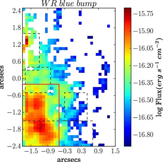
Emission map of the blue WR feature (created by integrating over the full emission feature from 4600 to 4700 Å), showing the distribution of WR stars in the FOV. The red rectangular box shows the peak of the WR distribution that we use for subsequent analysis. The four black dashed rectangular boxes denote the location of the four H ii regions. White spaxels correspond to the spaxels in which WR emission fluxes had S/N < 3.
Fig. 16 presents the WR ‘blue bump’ feature in integrated spectra of all H ii regions along with the WR region, which shows the peak in the WR distribution (red box in Fig. 15). In all these spectra, we find a gap between the broad 4640 feature and the [Fe iii] λ4658.05 emission line. This rare feature was first identified strongly in NGC 3049 (Schaerer, Contini & Kunth 1999) and explained as a real feature by Schmutz & Vacca (1999). Basically, the gap arises because the 4640 feature is not one broad feature but a combination of at least three emission components (N v λλ4604, 4620; N iii λλ4634, 4641; C iii λλ4647, 4650). Except region 4, none of the star-forming regions show a prominent WR ‘blue bump’ feature. Inspecting the spectra of region 4, we find the observed blue bump is mainly due to the common region which it shares with the WR region. Hence, we concentrate on the WR region for subsequent analysis of WR stars.
![WR ‘blue bump’ features (N v λ4620, N iii λ4640, and He ii λ4685) in the integrated spectra of all H ii regions along with the region showing the peak in WR distribution (red box in Fig. 15). The integrated spectra are normalized by the continuum in the respective region and then offset by 0.2 with respect to each other for better visibility. On the right-hand side above each spectrum, we show the average level of continuum (in units of 10−15 erg s−1 cm−2 Å−1) in the given wavelength range corresponding to each region in the same colour. The blue bump indicates the presence of late-type WN and WC stars. All these spectra also show a gap between the broad λ4640 feature and the nebular iron line [Fe iii] λ4658.05 Å.](https://oup.silverchair-cdn.com/oup/backfile/Content_public/Journal/mnras/476/3/10.1093_mnras_sty402/1/m_sty402fig16.jpeg?Expires=1750096609&Signature=DmBWM27PkbvEz1Kgprc491hzT0AiL2lC1MrYMORE627LfShLWo-~tiFw8wtanyXA4XFGXKwCTDlaShoyGDkMtl6bSAWOkjoRxx-OU6XzV1k8NuN9F~W0bCiBkgihWEWD-lEVUles8D~Sq-YHM8A-ZXFJPFCB-aThlODD0ohSpq-xntK4LOUpo-I2ByWwQPF6arGn7LFYy6pqSnxdxQQRtlEwlI8A8qfVk7Wn4W6EuC7FQWEqANa3D1mCQXMk33hpSW2q03udQtytojJwvfDt8ninZQ8ge6YdSpuZhEYNHxd9iF1e-9~2Rf0KmV-TJJ9Yv-dY1-mXEY9h3p44U3PpkA__&Key-Pair-Id=APKAIE5G5CRDK6RD3PGA)
WR ‘blue bump’ features (N v λ4620, N iii λ4640, and He ii λ4685) in the integrated spectra of all H ii regions along with the region showing the peak in WR distribution (red box in Fig. 15). The integrated spectra are normalized by the continuum in the respective region and then offset by 0.2 with respect to each other for better visibility. On the right-hand side above each spectrum, we show the average level of continuum (in units of 10−15 erg s−1 cm−2 Å−1) in the given wavelength range corresponding to each region in the same colour. The blue bump indicates the presence of late-type WN and WC stars. All these spectra also show a gap between the broad λ4640 feature and the nebular iron line [Fe iii] λ4658.05 Å.
We estimate the number of WR stars in the region showing the peak of the WR distribution (red box in Fig. 15) by fitting WR templates to the integrated spectrum of the corresponding region. Since the mean metallicity of the FOV (12 + log(O/H) = 8.23) is closer to that of LMC than the SMC [i.e. 12 + log(O/H) = 8.35 and 12 + log(O/H) = 8.03, respectively (Russell & Dopita 1992)], we use the WR LMC templates (Crowther & Hadfield 2006). The specific LMC templates are selected on the basis of the relative strength of different components of the WR blue and red bumps revealed by our spectrum. For modelling the red bump, both WC4 and WO templates are available. We did a χ2 minimization using the two templates separately for the red bump and found that the WC4 template produced a better fit. Moreover, our spectrum has a clear C |$\small {IV}\lambda$|5808 feature indicating the presence of WC4 stars, but no O |$\small {V}\lambda$|5990, a signature of WO stars. Hence, we selected WC4 template for the rest of the template fitting. For fitting the more complex blue bump, we selected the WN7-9 template over the WN5-6 template, because the relative strength of He |$\small {II}\,\lambda$|4686 and the broad emission ∼4640 Å in our spectrum are similar to WN7-9 template. We also include the WN2-4 template for modelling the N |$\small {V}\,\lambda \lambda$|4604, 4620 feature revealed in our spectrum. Finally, we perform a χ2-minimization using the above selected templates and simultaneously fit all spectral regions of interest, i.e. the red bump and the three clear features of blue bump (N v λλ4604, 4620; N iii λλ4634, 4641; He |$\small {II}\ \lambda$|4686). In χ2 minimization, we used the dispersion in the emission-free continuum region as the uncertainty on the input WR fluxes. We calculated the uncertainty on the number of WR stars obtained from a Monte Carlo simulation using the dispersion in the emission-free region. Hence, we estimate ∼125 ± 4 carbon-type (WC4) stars, ∼60 ± 20 late-type (WN7-9) stars, and ∼480 ± 50 early-type (WN2-4) stars. The corresponding fit is shown in Fig. 17 for both blue (left-hand panel) and red bump (right-hand panel). Cairós et al. (2012) reports WR signatures in the central region of NGC 4670 that approximately overlaps with our FOV, though there is no estimate of the number of WR stars available for comparison with our study. We have found ∼670 ± 50 WR stars over a region of 212 pc × 116 pc. Our density is lower (∼ a factor of 2) in comparison to another BCD Mrk 996, where ∼3000 WR stars are reported in an area of 4.6 × 10⁴ pc2 (James et al. 2009). However, these densities are higher in comparison to a nearby WR galaxy Mrk 178, where 20 WR stars are found in a region of ∼300 × 230 pc (Kehrig et al. 2013).
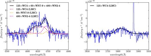
Left: Continuum-subtracted WR ‘blue bump’ feature summed over the peak of WR distribution (red box in Fig. 15). Overplotted is the combined fit (solid black curve) for 125 WC4 stars (red dashed curve), 60 WN7-9 stars (orange dashed curve), and 480 WN2-4 stars (magenta dashed curve), using the LMC templates of Crowther & Hadfield (2006). Right: Continuum-subtracted WR ‘red bump’ feature summed over the peak of WR distribution (red box in Fig. 15). Overplotted (solid black curve) is the scaled LMC template of WC4 star from Crowther & Hadfield (2006), denoting the presence of 125 WC4 stars.
3.5.3 Star formation rate
Assuming a constant metallicity throughout the FOV, we map the SFR at Z = 0.35 Z⊙ (Fig. 18), using the metallicity-dependent relation between dereddened luminosity of H α, L(H α), and SFR from Ly et al. (2016) derived from the Starburst99 models, assuming a Padova stellar track and Chabrier IMF (Chabrier 2003). The SFR values vary between 0.02 and 0.49 × 10⁻³ M⊙ yr−1 at sub-solar metallicity. We also map the SFR at solar-metallicity using the L(H α)–SFR relation, given in Kennicutt (1998) for a Salpeter IMF. We include a multiplicative factor of 0.63 in the SFR map at solar metallicity to account for the Chabrier IMF, which has a more realistic distribution at the lower end of stellar masses. We find that the SFR varies between 0.03 and 0.77 × 10⁻³ M⊙ yr−1 at solar metallicity. The SFR map at solar metallicity shows a similar pattern as the one at sub-solar metallicity.
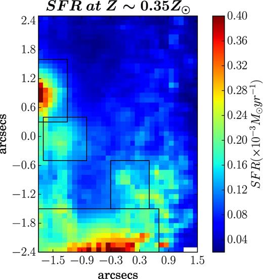
SFR map of the FOV in units of × 10−3 M⊙ yr−1 at 0.35 Z⊙. The four black rectangular boxes denote the location of the four H ii regions.
We also estimate the SFR for the four H ii regions at solar and sub-solar metallicities for each region using the recipes mentioned above. The results are given in Table 4. For both integrated data of the four H ii regions and spatially resolved data, we find that the SFR at sub-solar metallicity is lower than those at solar metallicity. This is because the atmosphere of metal-poor O stars are more transparent resulting in an increased escape fraction for the ionizing photons and hence lower SFR. Our results are in agreement with the SFRs of other BCDs, which span a range of 10−3–102 M⊙ yr−1 (Hopkins, Schulte-Ladbeck & Drozdovsky 2002).
4 DISCUSSION
4.1 N/O Conundrum revisited
The relationship between the nitrogen-to-oxygen ratio and the oxygen abundance in H ii regions has been the subject of intense debate (e.g. see McCall et al. 1985; Thuan et al. 1995; Henry et al. 2000; Izotov et al. 2006; López-Sánchez & Esteban 2010; Vincenzo et al. 2016; Belfiore et al. 2017) and has been used to probe the origin of nitrogen in different metallicity regimes. Based on the analysis of 54 H ii regions in BCDs, Izotov & Thuan (1999) proposed three metallicity regimes related to the origin of nitrogen. In the low-metallicity regime (12 + log(O/H) < 7.6), nitrogen is thought to have a primary origin and is produced by massive stars only, which set the level of log(N/O) at ∼ −1.6 with a very low scatter. However, since the mechanism of production of nitrogen in massive stars is not clearly understood, the behaviour of the relationship in the low-metallicity regime could also result due to effects related to stellar rotation (Meynet & Maeder 2005), low SFR (Henry et al. 2000), low number of WR stars (Izotov et al. 2006), or the production of nitrogen by low- and intermediate-mass stars (see e.g. López-Sánchez & Esteban 2010). In the intermediate-metallicity regime (7.6 < 12 + log(O/H) < 8.3), the value of log(N/O) increases above −1.6 and the origin of nitrogen is interpreted to be primary but produced by intermediate-mass stars, which evolve and release their nucleosynthesis products into the interstellar medium. The relation shows a large scatter (±0.3 dex). Berg et al. (2012) reports a positive slope between the log(N/O) and 12 + log(O/H) for the metallicity values 12 + log(O/H) > 7.7, indicating a secondary origin of nitrogen even in the intermediate-metallicity regime. However, their analysis of H ii regions in low-luminosity dwarf galaxies does show a large scatter. This scatter has been observed in several observational studies of systems with low and intermediate metallicities (e.g. van Zee & Haynes 2006; Pérez-Montero & Contini 2009; James et al. 2015, 2017), and has been attributed to factors such as the time delay between the production of oxygen and secondary nitrogen (Garnett 1990; Vila Costas & Edmunds 1993; Pettini et al. 2008), variation in the star formation histories (Mollá et al. 2006; Mollá & Gavilán 2010), the global gas flows in galaxies (Köppen & Hensler 2005; Amorín et al. 2012b). At high metallicities (12 + log(O/H) > 8.3), nitrogen is thought to have a secondary origin, and hence a positive slope is expected between log(N/O) and 12 + log(O/H). Interestingly, Kobulnicky & Skillman (1996) report a negative trend in the relation for H ii regions within the irregular starburst galaxy NGC 4214, with strong WR features.
In Fig. 19, we present the relationship between log(N/O) versus 12 + log(O/H) for the four H ii regions as well as the whole FOV (on spaxel-by-spaxel basis). We caution here that given the spatial scale of our data (∼9 pc), each spaxel may or may not host H ii regions, since the typical size of H ii regions varies between a few to hundreds of pc (Kennicutt 1984). The oxygen abundance and the nitrogen-to-oxygen ratio for the four H ii regions are calculated from the direct Te method. However, O/H and N/O for the spatially resolved data are estimated from the hii-chi-mistry code. For the four H ii regions, we compare these quantities calculated from the direct Te method and the hii-chi-mistry that included the use of [O iii] λ 4363 line. We find that they agree with each other within 1σ, except for the metallicity of one H ii region (region 4) that agrees within 2σ. As noted by Pérez-Montero (2014), there are dispersions of ∼0.2 dex in the hii-chi-mistry model-based and direct Te-method abundances. We expect no trend or a positive trend in these regimes as mentioned before. However, we find a hint of negative trend between N/O and O/H for the four H ii regions, while the negative trend is more prominent for the spatially resolved data (on spaxel-by-spaxel basis), covering 0.3 dex on y-axis and 0.6 dex on x-axis lying in the intermediate- and the high-metallicity regime. We find a correlation coefficient of −0.75 for the spatially resolved data.
![The relationship between log(N/O) versus 12 + log(O/H) for the four H ii regions as well as the whole FOV (on spaxel-by-spaxel basis). The four regions are colour-coded as follows: region 1: blue circle, region 2: green pentagon, region 3: red square, region 4: orange diamond. Smaller markers denote the spatially resolved (spaxel-by-spaxel) relation, where the two quantities [log(N/O) and 12 + log(O/H)] are calculated from the hii-chi-mistry code, whereas the bigger markers denote quantities calculated from the direct Te method for the four H ii regions. Magenta coloured markers denote the spatially resolved quantities of the regions of FOV excluding the four H ii regions. The median error bars for the spatially resolved quantities are shown in the right-hand corner.](https://oup.silverchair-cdn.com/oup/backfile/Content_public/Journal/mnras/476/3/10.1093_mnras_sty402/1/m_sty402fig19.jpeg?Expires=1750096609&Signature=GJnu3Rp-S5PqsbcVXkWshkxVk-e3lQQPZkRNBYDIJ7XcPFEYHaeqptGLyx2c0rWoBx1AOiVHtgFAuEKNm~AtCfDKo14hWgEWlAgVuyzbLXp1Ai-Wx6DJmUhoK-BE8rTwBW1GFvSFi3ZxWwEPfSuf~sV~G~DojiVkn-9lJyA~YYcKhOORFUHTg4uPGez1arIORoMwaP-BKbGg4KMAFmm8gjrXnLd9MUsFaNaIHintNZaF49mGIF~DjBh3~NKOZWXhpfIOAm0dx-i75SqUiz7PZMdTSviqZvrBtTkyk~-4RIansDPLNhK~wMtDEUInDUW6AJGxIWSTaY775QuwnelVaw__&Key-Pair-Id=APKAIE5G5CRDK6RD3PGA)
The relationship between log(N/O) versus 12 + log(O/H) for the four H ii regions as well as the whole FOV (on spaxel-by-spaxel basis). The four regions are colour-coded as follows: region 1: blue circle, region 2: green pentagon, region 3: red square, region 4: orange diamond. Smaller markers denote the spatially resolved (spaxel-by-spaxel) relation, where the two quantities [log(N/O) and 12 + log(O/H)] are calculated from the hii-chi-mistry code, whereas the bigger markers denote quantities calculated from the direct Te method for the four H ii regions. Magenta coloured markers denote the spatially resolved quantities of the regions of FOV excluding the four H ii regions. The median error bars for the spatially resolved quantities are shown in the right-hand corner.
As a sanity test, we also estimated the log(N/O) from the N2S2 calibration (Pérez-Montero & Contini 2009), and the metallicity from the N2 parameter (Pettini & Pagel 2004), and studied the relation. Since calibrations for N/O and O/H based on nitrogen lines (such as N2S2 and N2, respectively) in principle assume a positive relation between N/O and metallicity, we expected to see a change in the trend found using the direct measurements.For example, from Pérez-Montero & Contini (2009), their Figs 5 and 6 show the existence of a strong correlation between the metallicity derived from the N2 parameter and the N/O ratio in such a way that the metallicity predicted by N2 is overestimated in objects with a high N/O. However, we find that the apparent anticorrelation between N/O and O/H in Fig. 18 still holds, thereby adding confidence to our results. However, the slope (of the negative trend) in this case is steeper than that seen in the relation obtained using hii-chi-mistry. This might be due to the intrinsic increasing trend of N/O with metallicity in the secondary regime, which will pull the slope to show a positive slope, and hence will result in a steeper negative trend. In Fig. 19, we only show the spatially resolved relation based on quantities obtained from the hii-chi-mistry code rather than from indirect methods (N2 and N2S2), because the former is based on models that do not assume any relation between the metallicity and log(N/O). Moreover, the calibration uncertainty on indirect methods are very high (0.18 dex for (O/H)[N2] and 0.1 dex for (N/O)[N2S2] at 68 per cent confidence level), compared to hii-chi-mistry results. Given the spaxels are 0.1|${\rm \,arcsec}$|, one may also argue about the effects of seeing. However, seeing will only smear out any pre-existing trend rather than producing a non-existent trend. The slope of the spatially resolved data appears to be flatter than the slope of integrated data of the four H ii regions. This is likely due to the limitations of the photoionization models used in hii-chi-mistry as described in Pérez-Montero (2014). High S/N data allowing the detection of the weak auroral line would help circumvent this problem. From the S/N of the faintest H ii region (region 4), we estimate that we would need to stack around 20 spectra in order to achieve a S/N ([O iii] 4363) > 3.0 within this region. However, our tests on attempting to map this auroral line in the gaps between the H ii regions were not successful due to lack of S/N, even after integrating over 100 s of spaxels.
4.2 H ii regions in other BCDs
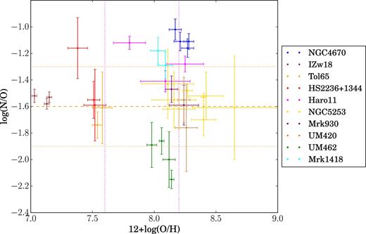
log(N/O) versus 12 + log(O/H) of H ii regions within BCDs, where data points in the same colour correspond to the H ii regions from the same BCD. See Table 5 for the data reference. The orange dashed line indicates the plateau at log(N/O) = −1.6, and the orange dotted lines correspond to ±0.3 dex enclosing the region of scatter found in the literature (e.g. Izotov & Thuan 1999). The vertical pink dotted lines at metallicity 12 + log(O/H) = 7.6 define the transition from low- to intermediate-metallicity regime and the transition from the intermediate-metallicity regime to the high-metallicity regime at 12 + log(O/H) = 8.2.
References and distances of the BCDs shown in Fig. 20.
| BCDs | References | Distance (Mpc) |
|---|---|---|
| NGC 4670 | This study | 18.6 |
| IZw18 | Kehrig et al. (2016) | 18.2 |
| Tol 65 | Lagos et al. (2016) | 42.7 |
| HS2236+1344 | Lagos et al. (2014) | 79.7 |
| Haro11 | James et al. (2013b) | 83.6 |
| NGC 5253 | Westmoquette et al. (2013) | 3.8 |
| Mrk930 | Pérez-Montero et al. (2011) | 83.2 |
| UM420 | James et al. (2010) | 23.8 |
| UM462 | James et al. (2010) | 14.4 |
| Mrk1418 | Cairós et al. (2009) | 14.6 |
In the sample of 10 galaxies, we first analyse six galaxies individually for which there are more than two data points. The values of the Pearson correlation coefficient ρ (Table C1) suggest a negative correlation for all the six galaxies. Taking error bars into account, we also fitted a constant model with and without any slope to perform a likelihood ratio test. In Appendix C, we present the values of ρ and the details of the log likelihood ratio test for six galaxies in the sample. Amongst the six galaxies, IZw 18 and HS2236+1344 lie in the low-metallicity range where we would not expect a trend, which is also shown by the likelihood ratio test. For NGC 4670, ρ = −0.83, which suggests a strong anticorrelation. However the likelihood ratio test does not favour a negative trend for the group of Hii regions under study. Out of the remaining three galaxies, the likelihood ratio test shows that two BCDs in the samples Haro 11 and UM 462 exhibit a negative trend.
The above analysis cannot be performed on the remaining four galaxies (Mrk1418, Mrk930, UM420, and Tol 65) that have only two data points. However for one of the two regions in Tol 65, Lagos et al. (2016) report high spatially resolved log(N/O) values, preferentially in spaxels with lower oxygen abundance, which indicates a negative trend on spaxel-by-spaxel basis.
Though in the above analysis we have found hints of a negative trend in the log(N/O) versus log(O/H), it is difficult to say anything definite about the trend because of the few data points in each galaxy. To circumvent this problem, we put the data points corresponding to each galaxy on the same scale of metallicity and log(N/O) by normalizing them with the medians of the metallicities and log(N/O) for all H ii regions in the 10 BCDs. Fig. 21 shows the relation after normalization. We find a negative correlation coefficient of ρ = −0.50. While the trend was not at all clear from the scatter plot of Fig. 20, there is a strong hint of a negative trend in Fig. 21. The likelihood ratio test also confirms the negative trend (see Appendix C). The negative slope (−0.6 ± 0.16) that we find here agrees within errors with the slope (−0.798 ± 0.350) found for NGC 4214 (Kobulnicky & Skillman 1996). This shows that it is quite possible that a negative trend between log(N/O) and metallicity might exist for H ii regions within BCDs.
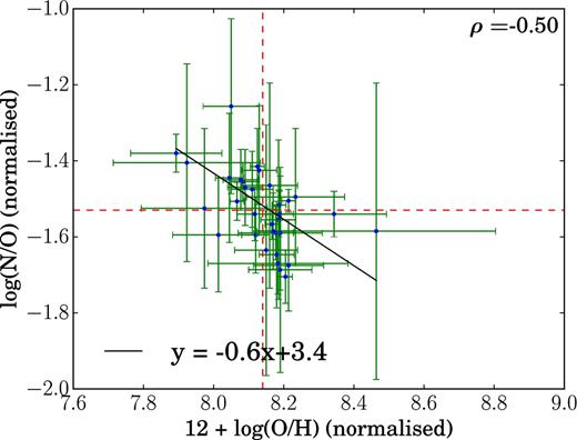
Normalized log(N/O) versus 12 + log(O/H). Error bars are the same as on the original data points (as in Fig. 20). Best fit: y = (−0.6 ± 0.16)x + (3.4 ± 1.3). The red dashed straight lines correspond to the medians of the log(N/O) and 12 + log(O/H).
4.3 Possible causes for a negative relation between N/O and O/H
In this section, we discuss possible explanations for a negative trend between metallicity and log(N/O) in spatially resolved data. In order to understand the negative trend, we need to put our spatially resolved data of NGC 4670 in a more global perspective. Fig. 22 shows our spatially resolved data from this study (brown points) along with the global data (grey points) of a galaxy sample drawn from the MPA-JHU catalogue of SDSS Data Release 7 including only objects classified as purely star forming. They lie in the redshift range of 0.023 < z < 0.1 and their stellar masses are restricted to 7 <log(M⋆/M⊙) ≤ 9 because BCDs are dwarfs with a stellar mass M⋆ < 109 M⊙ (Lian et al. 2016). We compute the log(N/O) and log(O/H) for SDSS galaxies using the hii-chi-mistry code. In Fig. 22, we find that the higher metallicity and lower (N/O) end overlaps with the normal star-forming galaxies and therefore is experiencing the typical gas mixing observed within this metallicity range. The deviation occurs for the metallicity range 12+log(O/H) ≲ 8.2.
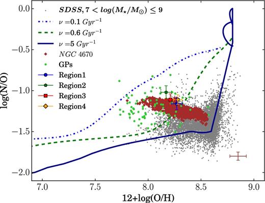
Chemical evolution models from Vincenzo et al. (2016) on the log(N/O) versus log(O/H) plane. The three curves correspond to the three different SFEs, i.e. ν = 5 Gyr−1 (solid blue), ν = 0.6 Gyr−1 (dashed green), and ν = 0.1 Gyr−1. These models are generated at the infall mass of 109 M⊙ and Kroupa IMF. The data corresponding to the integrated spectra of the four star-forming regions are obtained from the direct Te method and are colour coded as in the previous figures – region 1: blue, region 2: green, region 3: red, and region 4: orange. The spatially resolved data from this work are shown as brown points with the median error bars at the right-hand corner of the plot. The SDSS DR7 data for a sample of nearby star-forming galaxies are shown by grey dots, and the data for green peas are shown by light green points. The hii-chi-mistry code has been used to generate the values of log(N/O) and log(O/H) for spatially resolved data from this work, SDSS galaxies, and the green peas.
Relation to star formation activity and localized N enrichment: To explain the deviation observed in Fig. 22, we show in Fig. 23 the spatially resolved relation between log(N/O) versus 12 + log(O/H), obtained from the hii-chi-mistry as explained in Section 3.4.2. The data points are colour-coded with respect to the intrinsic H α fluxes in the corresponding spaxels. Since H α traces the current (<5 Myr) star formation activity, we use the intrinsic H α flux as a proxy for the ongoing star formation activity in the region of interest. We did not utilize the spatially resolved SFR maps created in Section 3.5.3 because the SFR recipes used to create these maps assume a certain metallicity (solar or sub-solar). Though the metallicity dependence will only act as an additive constant in Fig. 23, we prefer avoiding any circularity of argument in the analysis. In Fig. 23, we find that the spaxels with higher metallicity and lower log(N/O) show a lower intrinsic H α flux, whereas the spaxels with lower metallicity and higher log(N/O) show a higher intrinsic H α flux.
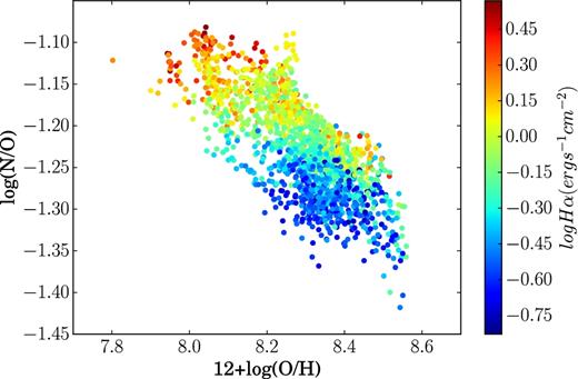
Spatially resolved relationship between log(N/O) and 12 + log(O/H), where data points are obtained from hii-chi-mistry code and are colour-coded with respect to the intrinsic H α fluxes in the corresponding spaxels. We find that the spaxels with lower metallicity and higher log(N/O) also show higher H α fluxes, whereas the spaxels with higher metallicity and lower log(N/O) show lower H α fluxes. H α being a proxy for current (<5 Myr) star formation, the negative trend in the log(N/O) versus metallicity is apparently dependent on the ongoing star formation.
At the low-metallicity end, the trend between low metallicity and increased star formation can be explained by a scenario in which metal-poor gas flows in, increasing the SFR of the region and decreasing the metallicity. The velocity map of the FOV (Fig. 7, left-hand panel) shows a rotating structure, with no shock or turbulence that is typical of inflow/outflow. However, gas flows have been proposed/studied in galaxies with indication of rotation (Queyrel et al. 2012; Sánchez Almeida et al. 2014, 2015; Olmo-García et al. 2017), which may be the case in NGC 4670. A possible cause of the high log(N/O) is a localized nitrogen enrichment of the interstellar medium from the ejecta of WR stars (Kobulnicky et al. 1997; Brinchmann, Kunth & Durret 2008; López-Sánchez & Esteban 2010). In support of this enrichment scenario, the log(N/O) map (Fig. 11) also shows an increase in the region approximately coincident with the peak in WR emission (Fig. 15). Note here that if metal-poor gas were inflowing, the level of nitrogen enrichment needed to produce an elevated log(N/O) for a given low log(O/H) would be significant. Note here that the inflow does not change N/O at all, only changes O/H. Even if the inflow dilutes the metallicity by say 0.2 dex, the N/O is still larger than the spaxels with that metallicity. Hence, pollution seems certainly more likely than inflow in this case because the N/O enhancement seems local.
Varying star formation efficiency (SFE) in different star-forming regions: In Fig. 22, we also show the chemical evolution models (three curves) taken from Vincenzo et al. (2016). Though these models have been originally tested on a global basis for galaxies (SDSS sample and low-metallicity dwarfs), they can be used for our spatially resolved data. This is because in these models, it is assumed that a galaxy is made up of a single zone within which the chemical elements mix instantaneously and uniformly. This assumption is valid for individual star-forming regions as well. Note here that no chemical evolution models are available currently for studies inside galaxies at spatially resolved scales; hence, these models provide the best alternative for the spatially resolved study presented here. Details on these models can be found in Vincenzo et al. (2016) and Matteucci (2012) including their specific parameters such as infall mass (Minf), infall time-scale, star formation efficiency (SFE denoted by ν), IMF, mass loading factor, differential galactic outflow.
While employing the chemical evolution models, we have assumed the reference values for all parameters given in Vincenzo et al. (2016), except Minf and SFE. Since the BCDs are low-mass galaxies, we have assumed Minf = 109 M⊙. At the infall time-scale of τinf = 0.1 Gyr and Kroupa IMF (Kroupa, Tout & Gilmore 1993), we vary SFEs from 0.1 to 5 Gyr−1, shown by three curves with the purpose of covering the region on the plot occupied by the spatially resolved data of NGC 4670. We find that the spaxels with higher log(N/O) and lower metallicity lie on the region in the plot covered by the chemical evolution model with a relatively low SFE, i.e. ν ∼ 0.1 Gyr−1. However, the spaxels with lower log(N/O) and higher metallicity lie in that region that is covered by the models with a relatively high SFE, i.e. ν ∼ 5 Gyr−1. The curve corresponding to an intermediate value of SFE appears to go through the middle of the distribution of (N/O)-(O/H) values. Hence, we find a gradient in SFE while going from one end [high (N/O)-low (O/H)] to the other end [low (N/O)-high (O/H)] of (N/O)–(O/H) plane. A higher SFE will result in an increased production of oxygen per unit time by massive stars increasing the metallicity of the corresponding regions. If there is a delay in the production of nitrogen, the ratio of nitrogen-to-oxygen will decrease. The same argument related to the delayed production of nitrogen can be applied to the regions with lower SFE, low-metallicity, and high nitrogen-to-oxygen ratio. Hence, it appears that the SFE at small spatial scales plays an important role in maintaining the oxygen abundance and the nitrogen-to-oxygen ratio within galaxies. It is likely through its effect on the star formation history and on the balance of the different stellar population that contribute to the oxygen and nitrogen abundance (Vincenzo et al. 2016).
However, this scenario does not tie in easily with the increased H α at high log(N/O) and low metallicity. An increased H α indicates a higher SFR, while the same regions are covered by lower SFE as seen in Fig. 22. This indicates a higher SFR in a region with lower SFE. If we define SFE as the ratio of SFR to the available gas for forming stars, then a high SFR for a region with lower SFE simply implies that a large amount of gas is available in the region that is not forming stars. To explore this hypothesis, a more complete analysis of the spatial distribution of the relative abundance of neutral, molecular, and ionized gas are required. High SFR with low SFE may also point towards the fact that star formation is a self-regulating process at local sub-galactic scales. Regions with high SFRs may have strong negative energetic feedback from the massive dying stars, which will result in a decreased SFE in the respective star-forming regions.
Alternative explanation: In Fig. 22, we also show data corresponding to green pea galaxies that are low-redshift extreme emission-line galaxies with very high specific SFR that are also thought to be excellent analogues of high-redshift star-forming galaxies (Cardamone et al. 2009). As we can see in Fig. 22, they exhibit relatively high log(N/O) at a given metallicity in the low-to-intermediate metallicity regime compared to the SDSS galaxies. As discussed in Amorín et al. (2010, 2012a), the possible cause of such a behaviour could be the simultaneous inflow of metal-poor gas induced by interactions and the outflow of metal-rich gas driven by supernova remnants and stellar winds. The scenario involving gas dynamics was proposed by other observational (van Zee, Salzer & Haynes 1998) and theoretical studies (Köppen & Hensler 2005) as well. In our study, we have found a relative increase in the He abundance in the region of NGC 4670 surrounding and the WR bump, which suggests the local effect of a strong wind emanating from the WR stars. The age of the stellar population found in our work is 10–30 Myr, which are old enough for the existence of supernova remnants and stellar winds from them. Further analysis is required to find the dynamical state of the ionized, molecular, and neutral gas in this galaxy.
5 SUMMARY
We have carried out a spatially resolved study of four H ii regions and the surrounding ionized gas located in the central region of the BCD NGC 4670 using the GMOS-N IFS data at the spatial scale of 9 pc. A summary of our main results is as follows:
The radial velocity map indicates a slow rotation of the ionized gas varying between ∼ −10 and 30 km s−1 about an isovelocity S-shaped contour. The velocity dispersion varies between 40 and 104 km s−1, with relatively lower dispersion in the H ii regions. No signatures of shock or complex velocity structure is found. The classical [S ii]/H α and [N ii]/H α emission-line ratio or BPT diagrams show that photoionization by massive stars is the main source of ionization.
In the integrated spectra of the four H ii regions, we could detect the auroral lines [O iii] λ4363, [O iii] λλ7320, 7330 that we use to estimate Te ([O iii]), Ne ([S ii]) and Te ([O ii]), and hence calculate 12 + log(O/H) varying between 8.17 and 8.28, log(N/O) varying between −1.02 and −1.16, and the helium abundance y+(5876) varying between 0.086 and 0.093 for the four Hii regions.
In the spatially resolved data of the FOV, the auroral line [O iii] λ4363 could not be detected with enough S/N (>3), which prevented the chemical abundance determination using the direct Te method. Hence, we use the hii-chi-mistry (v3.0) to map 12 + log(O/H) and log(N/O), which vary between 7.80 and 8.56 and between −1.4 and −1.08, respectively, across the FOV. We then use the 12+log(O/H) map to create Te and Ne maps, with which we map helium abundance y+(5876) varying between 0.05 and 0.12.
The age map is created at a metallicity of 0.35 Z⊙ by comparing the observed EW(H α) map with the modelled EW map using the starburst99 population synthesis model. The resultant age map varies between 10 and 30 Myr.
We also estimate the number of WR stars from the integrated spectrum of the WR region, which overlaps with three of four H ii regions. The WR region contains approximately ∼125 ± 4 WC4 stars, ∼60 ± 20 WN7-9 stars, and ∼480 ± 50 WN2-4 stars. The estimate is done by using the LMC WR templates from Crowther & Hadfield (2006).
We map SFR of the FOV from the dereddened H α luminosity at sub-solar metallicity of 0.35 Z⊙ that varies between 0.02 and 0.49 × 10⁻³ M⊙ yr−1.
We revisit the N/O conundrum by studying the relation between the spatially resolved 12 + log(O/H) and log(N/O) and the integrated data of the H ii regions from 10 other BCDs from the literature and found an unexpected negative trend. We also compare the spatially resolved data with the low-mass SDSS galaxies and the green pea galaxies and explore various scenarios to explain the trend including nitrogen enrichment, and variations in SFE via chemical evolution models.
In summary, the present analysis shows that a negative trend between log(N/O) and 12+log(O/H) may exist at the spatially resolved scales and H ii regions within BCDs. It is possible that the negative trend that we observe in our spatially resolved data is merely a manifestation of the large scatter that has been observed previously in other low-metallicity galaxies. To confirm the behaviour of log(N/O) with metallicity, these two properties and their relation need to be studied with high S/N data at spatially resolved scales across a large sample of BCDs. Those data sets would allow us to map the distribution of metallicity and log(N/O) from robust direct methods and also analyse the WR population in the entire galaxy for a plausible effect of chemical pollution. Moreover, such data sets would enable the study of variation of the above-mentioned observables not only within galaxies but also within H ii regions, for example via radial profile analysis or a segmentation analysis of individual H ii regions (López-Hernández et al. 2013). Those studies would be possible in the future with the current and upcoming IFS facilities like MUSE on Very Large Telescope, WEAVE on William Herschel Telescope, and Keck Cosmic Web Imager because of their large FOV and good spatial sampling, which will enable us to map chemical abundances of entire galaxies. Moreover, such studies could also investigate kinematic signatures to further probe the possible cause of the observations related to gas dynamics. As we have shown here, the combination of chemical and kinematical analyses is essential in disentangling chemical evolution scenarios, and obtaining such information across a large sample of entire systems will be key in understanding the origin of nitrogen in these less chemically evolved star-forming systems. In so doing, we will enhance our understanding of chemical evolution scenarios in galaxies within the high-redshift Universe.
ACKNOWLEDGEMENTS
This study is based on observations obtained at the Gemini Observatory (processed using the Gemini iraf package), which is operated by the Association of Universities for Research in Astronomy, Inc., under a cooperative agreement with the NSF on behalf of the Gemini partnership: the National Science Foundation (USA), the National Research Council (Canada), CONICYT (Chile), Ministerio de Ciencia, Tecnología e Innovación Productiva (Argentina), and Ministério da Ciência, Tecnologia e Inovação (Brazil). It is a pleasure to thank Jose Vilchez for various useful discussions during the course of this work. We also thank Alessandra Aloisi, Tracy Beck, and Mark Westmoquette for their invaluable help during the early stages of this project. N.K. thanks Fiorenzo Vincenzo for providing with the chemical evolution models. We thank the referee for a positive feedback. N.K. thanks the Institute of Astronomy, Cambridge and the Nehru Trust for Cambridge University for the financial support during her PhD. B.L.J. thanks support from the European Space Agency (ESA). R.A. acknowledges the support from the ERC Advanced Grant 695671 QUENCH. E.P.M. thanks financial support from Spanish MINECO project AYA2016-797124-C4-4-P and CSIC grant EPM461-201650I042 and Kavli Institute for Cosmology in Cambridge for kindly hosting him in July 2017 when part of this work was made. This research made use of the NASA/IPAC Extragalactic Database (NED) that is operated by the Jet Propulsion Laboratory, California Institute of Technology, under contract with the National Aeronautics and Space Administration; SAOImage DS9, developed by Smithsonian Astrophysical Observatory; and astropy, a community-developed core python package for Astronomy (Astropy Collaboration et al. 2013).
Footnotes
iraf is distributed by the National Optical Astronomy Observatory, which is operated by the Association of Universities for Research in Astronomy (AURA) under a cooperative agreement with the National Science Foundation.
The choice of attenuation curves is of little importance here as the attenuation curves of LMC, Small Magellanic Cloud (SMC), starburst, or the Milky Way (MW) have similar values in the optical range.
One may also estimate the thermal contribution to the velocity dispersion (Amorín et al. 2012b). From the mean Te values of the four H ii regions (Table 4), we estimated this contribution as |$\sqrt{\frac{kT_{\rm e}}{m_H}}$| ∼ 9 km s−1. This correction leads the velocity dispersion to decrease by only ∼1 km s−1.
See Appendix A for updated formulae.
The maps of Te ([O iii]) and Ne derived in this section are presented in Appendix B.
Taking the ratio of summed fluxes of WR map with S/N > 3 and summed fluxes of [Fe iii] λ4658 with S/N > 1, we find an upper limit of 6 per cent as contribution of [Fe iii] λ4658 in the WR map.
REFERENCES
APPENDIX A: FORMULAE
We present here some of the formulae used in this work, which are actually taken from Pérez-Montero (2017), but have some misprints in the published version. The correct expressions are as follows:
- Temperature of low-ionization zone:where(A1)\begin{equation} t([{\rm O}{\small II}]) (10^4\,{\rm K}) = a_0(n) + a_1(n)R_{{\rm O}2} + \frac{a_2(n)}{R_{{\rm O}2}}, \end{equation}(A2)\begin{equation} R_{{\rm O}2} = \frac{ I(3726\,{\rm \mathring{\rm A} }) + I(3729\,{\rm \mathring{\rm A} }) }{ I(7319\,{\rm \mathring{\rm A} }) + I(7330\,{\rm \mathring{\rm A} }) } \end{equation}(A3)\begin{equation} a_0 (n) = 0.2526 - 0.000357n - \frac{0.43}{n} \end{equation}(A4)\begin{equation} a_1 (n) = 0.00136 + 5.431\times 10^{-6} n + \frac{ 0.00481 }{ n } \end{equation}(A5)\begin{equation} a_2 (n) = 35.624 - 0.0172 n + \frac{25.12}{ n }. \end{equation}
- The ratio N+/O+where tl is the low-ionization zone temperature in units of 104 K.(A6)\begin{eqnarray} {\rm log}(\frac{{\rm N}^+ }{ {\rm O}^+ }) &=& {\rm log}( \frac{I(6583)}{I(3726) + I(3729)})+ 0.493 - 0.025t_l \nonumber\\ &-& \frac{0.687}{t_l} + 0.1621{\rm log}(t_l), \end{eqnarray}
APPENDIX B: ELECTRON TEMPERATURE AND DENSITY DERIVED FROM METALLICITY
Fig. B1 (upper panel) shows the Te([O iii] map obtained from the metallicity map (Fig. 10), which was itself derived from the hii-chi-mistry code. Using this indirectly obtained Te map and the [S ii] doublet ratio, we derived the Ne map (Fig. B1, lower panel). We find that the majority of spaxels show 50 cm−3, which is actually an upper limit on the electron density. This shows that the region under study is low-density region.
![Upper panel: Te([O iii] map obtained from the metallicity map (Fig. 10). Lower panel: Ne map using the [S ii] doublet ratio map and Te([O iii] map on left. Majority of the spaxels have upper density limit of 50 cm−3 in those spaxels. The four rectangular boxes in the two maps show the location of the four H ii regions.](https://oup.silverchair-cdn.com/oup/backfile/Content_public/Journal/mnras/476/3/10.1093_mnras_sty402/1/m_sty402figb1.jpeg?Expires=1750096609&Signature=euJ1VrYdW0M7IUDgM8tu3KubYJ9i8FPWkdoxFJozD2yT8IHtcsPOGwLhczFMS502M-mVVy4Mq0aVy0feLplYv3sMcjv5UBblWEzQPYdUKXdQ8pp88fvTfHrAy-FnwAykBrsmXZWJDnq9JTaGv77RcFWqmhJonxP1jL9F3kGtewRMmDiEs3zgWvsTapOwQ4J8QPCRZxDyRjg1oIi33tlXTlRf9D-J9kZuWU6wSw6jbGoK--YEv23h3qiihShu3X2JSEHlKEtzTzuvTTE1pGvkJ6cgF2E5Gx6fxtf8FZVg8KVxw0au6nv8a7gZv4oIOAhqnR1dpcevUZ6F0c36FCfcLQ__&Key-Pair-Id=APKAIE5G5CRDK6RD3PGA)
Upper panel: Te([O iii] map obtained from the metallicity map (Fig. 10). Lower panel: Ne map using the [S ii] doublet ratio map and Te([O iii] map on left. Majority of the spaxels have upper density limit of 50 cm−3 in those spaxels. The four rectangular boxes in the two maps show the location of the four H ii regions.
APPENDIX C: ANALYSIS OF LOG(N/O) VERSUS 12 + LOG(O/H) FOR H ii REGIONS WITHIN BCDs
The correlation coefficient for the six galaxies are given in Table C1.
Pearson correlation coefficient for individual galaxies.
| Galaxy | ρ |
|---|---|
| NGC4670 | −0.83 |
| IZw18 | −0.50 |
| HS2236+1344 | −1.00 |
| Haro11 | −0.68 |
| UM462 | −0.79 |
| NGC5253 | −0.45 |
| Galaxy | ρ |
|---|---|
| NGC4670 | −0.83 |
| IZw18 | −0.50 |
| HS2236+1344 | −1.00 |
| Haro11 | −0.68 |
| UM462 | −0.79 |
| NGC5253 | −0.45 |
We performed the likelihood ratio test (Neyman–Pearson test) for 6 out of 10 BCDs to find out if there exists a negative trend between log(N/O) and log(O/H) for H ii regions within BCDs. For each BCD, we fit two straight lines of the form: y = c and y = mx + c, where m is the negative slope and c is the constant. The individual straight line fits for the six galaxies are shown in Fig. C1. All these fits take into account the error bars on the fitted data. The corresponding χ2 values are tabulated in Table C2. |$\chi ^2_{y\,=\,c} - \chi ^2_{y\,=\,mx\,+\,c}$| is known to follow a |$\chi _1^2$| distribution. Since for a χ2 distribution, variance(χ2) = σ2 = 2ν; hence, we have |$\sigma = \sqrt{2}$|. The results of the test are shown in Table C2. We find that a straight line of the form y = c, fits four out of six galaxies that includes NGC 4670. Only two galaxies Haro 11 and UM462 show a negative trend. The results of the likelihood ratio test on the normalized data for all H ii regions (Fig. 21) are shown in the last column, which show that a negative correlation exits between log(N/O) and log(O/H).
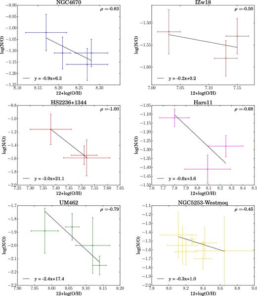
The individual straight line fits for the six galaxies, which have more than two data points. The best-fitting parameters is shown at the bottom-left corner in each panel, where y denotes log(N/O) and x denotes 12 + log(O/H). The Pearson correlation coefficient is shown in the top right corner of each panel, which is negative for six galaxies.
Likelihood ratio test fit for individual galaxies.
| Galaxy | |$\chi ^2_{y\,=\,c}$| | |$\chi ^2_{y \,= \,mx\,+\,c}$| | |$\chi ^2_{y\,=\,c}$| − |$\chi ^2_{y\, =\, mx+c}$| | |$\frac{\chi ^2_{y\, = \,c} - \chi ^2_{y\,=\,mx+c}}{\sigma }$| | |
|---|---|---|---|---|---|
| NGC4670 | 1.758 | 0.713 | 1.045 | 0.7 | |
| IZw18 | 1.152 | 0.961 | 0.191 | 0.1 | |
| HS2236+1344 | 2.340 | 0.001 | 2.339 | 1.7 | |
| Haro11 | 10.592 | 5.381 | 5.211 | 3.7 | |
| UM462 | 6.517 | 1.560 | 4.957 | 3.5 | |
| NGC5253 | 3.554 | 3.122 | 0.432 | 0.3 | |
| 10 galaxies | 31.896 | 23.085 | 8.811 | 6.2 |
