


Abstract
Direct collapse within dark matter haloes is a promising path to form supermassive black hole seeds at high redshifts. The outer part of this collapse remains optically thin. However, the innermost region of the collapse is expected to become optically thick and requires to follow the radiation field in order to understand its evolution. So far, the adiabatic approximation has been used exclusively for this purpose. We apply radiative transfer in the flux-limited diffusion (FLD) approximation to solve the evolution of coupled gas and radiation for isolated haloes. We find that (1) the photosphere forms at 10−6 pc and rapidly expands outwards. (2) A central core forms, with a mass of 1 M⊙, supported by gas pressure gradients and rotation. (3) Growing gas and radiation pressure gradients dissolve it. (4) This process is associated with a strong anisotropic outflow; another core forms nearby and grows rapidly. (5) Typical radiation luminosity emerging from the photosphere is 5 × 1037–5 × 1038 erg s−1, of the order the Eddington luminosity. (6) Two variability time-scales are associated with this process: a long one, which is related to the accretion flow within the central 10−4–10−3 pc, and 0.1 yr, related to radiation diffusion. (7) Adiabatic models evolution differs profoundly from that of the FLD models, by forming a geometrically thick disc. Overall, an adiabatic equation of state is not a good approximation to the advanced stage of direct collapse, because the radiation is capable of escaping due to anisotropy in the optical depth and associated gradients.
1 INTRODUCTION
A growing number of quasars found at redshifts z ≳ 6, including one at z ∼ 7.54 (Venemans et al. 2017; Banados et al. 2018), when the universe was younger than a gigayear, requires a very efficient way of forming early supermassive black holes (SMBHs; e.g. Fan et al. 2003; Willott et al. 2010; Mortlock et al. 2011; Wu et al. 2015). While small black holes can form just after the Big Bang (e.g. Carr et al. 2010), SMBHs must wait until the gas can collapse within dark matter (DM) haloes. SMBH seeds can form as the end products of stellar evolution, namely of metal-free Population III stars (e.g. Haiman & Loeb 2001; Abel, Bryan & Norman 2002; Bromm & Larson 2004; Volonteri & Rees 2006; Li et al. 2007; Pelupessy, Di Matteo & Ciardi 2007), supermassive stars (SMS; e.g. Haehnelt & Rees 1993; Bromm & Loeb 2003; Begelman, Volonteri & Rees 2006; Wise, Turk & Abel 2008; Begelman & Shlosman 2009; Milosavljević et al. 2009; Regan & Haehnelt 2009; Schleicher, Spaans & Glover 2010; Hosokawa et al. 2011; Choi, Shlosman & Begelman 2013, 2015; Latif et al. 2013a,b; Shlosman et al. 2016), and stellar clusters, either relativistic (e.g. Ipser 1969) or gas rich (e.g. Devecci & Volonteri 2009; Lupi et al. 2014). In principle, it is also possible that the stellar evolution stage can be by-passed completely, for example if the gas never gets hot enough to ignite thermonuclear reactions (e.g. Begelman & Shlosman 2009; Choi et al. 2013; Shlosman et al. 2016).
In this work, we focus on direct collapse scenarios, in which gas accumulates and collapses to form an SMBH seed either with or without the intermediate stage of an SMS. Such models are often glossed over an important stage in the collapse, when it becomes optically thick, substituting an adiabatic approximation for a detailed study of the radiation hydrodynamics.
Direct collapse can happen only when the virial temperature of DM haloes exceeds the gas temperature. If the gas with a primordial composition is capable of forming molecular hydrogen, haloes with virial temperatures of ∼100–1000 K can suffice. In this case, gravitational collapse leads to one or a few Population III stars per halo for z ≲ 50, with an initial mass function (IMF) initially thought to be top-heavy, ∼100–1000 M⊙ (e.g. Abel et al. 2002; Bromm et al. 2002; O'Shea & Norman 2007; Bromm 2013). Inclusion of radiative feedback indicates a rather normal IMF (e.g. Hosokawa et al. 2011; Hirano et al. 2015; Hosokawa et al. 2016). Supersonic streaming velocities remaining from recombination can suppress formation of Population III stars, allowing the gas to form a more massive central object (Hirano et al. 2017).
If, however, the Population III stars dissociate H2 or prevent its formation altogether, collapse will be triggered only for virial temperatures T ≳ few × 103 K. Suitable haloes have masses of 107–108 M⊙ and become abundant at z ≲ 20. Under these latter conditions, it has been conjectured that direct collapse will lead to an SMS with a mass in the range of ∼104–106 M⊙, if fragmentation can be suppressed and the angular momentum can be efficiently transferred out.
Begelman & Shlosman (2009) argued that gravitational torques transfer the angular momentum in the collapsing gas to the DM and the outer gas, which has been verified explicitly, both for isolated collapse and collapse in a cosmological framework (Choi et al. 2013, 2015). Furthermore, they found that global instabilities in the rotating collapsing gas lead to supersonic turbulent motions that damp fragmentation in the atomic gas. Contrary to self-similar analysis, which was necessarily limited to a linear stage (Hanawa & Matsumoto 2000), the growing bar-like m = 2 mode in its nonlinear stage did not lead to fragmentation, but induced gas inflow. In all cases, the collapse is dominated by filamentary structure (e.g. Luo et al. 2016; Shlosman et al. 2016).
The final stages of the collapse are expected to be characterized by radiation trapping, initially partial and thereafter complete. Simple logic points to the formation of a central object, but its nature is elusive. Is the collapse stopped early, leading to the formation of a hydrostatic object, an SMS, whose subsequent evolution leads to the formation of the SMBH seed? Or can the collapse proceed directly to an SMBH seed?
If the SMS forms, it has been conjectured that the follow-up nuclear burning and core collapse leave an SMBH seed of ∼10–105 M⊙, which grows rapidly via hypercritical accretion. Such a pre-collapse object has the structure of a hylotrope, and the post-collapse configuration has been termed a quasi-star (e.g. Begelman, Volonteri & Rees 2006; Begelman, Rossi & Armitage 2008; Begelman 2010).
The formation details of the SMS, however, appear to be murky. When does the photosphere form and where, what is its shape, and what is the effective temperature? How does an SMS get rid of the angular momentum in the collapsing gas? Does it rotate as a star, i.e. with surfaces of constant angular momentum, J, that resemble ellipsoids of rotation? Or does it rotate as a disc, i.e. with iso-J surfaces of a cylindrical shape? Are the central conditions sufficient to trigger thermonuclear reactions? How efficient is convection? Is the formation of the SMS associated with radiation- or gas pressure-driven outflows?
Models of the optically thin part of the collapse within DM haloes, on scales of ∼1 kpc down to ∼1 au, have emphasized various aspects of this stage: from formation and effects of molecular hydrogen, to Ly α diffusion, to background UV flux produced by Population III stars, as we have referenced above. However, inside ∼1 au, the radiation pressure is expected to build up, and have both dynamical and thermodynamical effects. Current modelling assumes that the radiation pressure build-up within the optically thick flow will lead it to follow an adiabatic equation of state (e.g. Becerra et al. 2015, 2017).
In this work, we test this assumption by treating the optically thick part of the accretion flow using radiative transfer in the flux-limited diffusion (FLD) approximation. We follow the flow as the radiation pressure builds up and becomes as important as the gas thermal pressure. Moreover, we evolve the adiabatic models to compare and contrast with the model involving radiative transfer. In the current paper, we deal with an isolated DM halo, while in the accompanying paper (Ardaneh et al. 2018), we invoke DM haloes within a fully cosmological framework.
This paper is structured as follows. The next section describes the numerical aspects of our modelling, the details of radiation transfer solver implemented here, and the initial conditions used. Sections 3 and 4 present our results for adiabatic and non-adiabatic flows, respectively, and Section 5 compares them. The last section summarizes our main conclusions from this work. We provide test models for radiative transfer in the Appendix. In the following, we abbreviate spherical radii with R and cylindrical ones with r.
2 NUMERICAL TECHNIQUES
We use the modified version of the Eulerian adaptive mesh refinement (AMR) code Enzo-2.4 (Bryan & Norman 1997; Norman & Bryan 1999). Our modifications are explained in this section.
Enzo uses a multigrid particle mesh N-body method to calculate gravitational dynamics including collisionless DM particles, and a second-order piecewise parabolic method (Colella & Woodward 1984; Bryan et al. 1995) to solve hydrodynamics. The structured AMR used in Enzo allows additional inner meshes as the simulation advances to enhance the resolution in the user-desired region. It places no fundamental restrictions on the number of rectangular grids used to cover some region of space at a given level of refinement, or on the number of levels of refinement (Berger & Colella 1989). A region of the simulation grid is refined by a factor of 2 in length scale, if the gas or DM densities become greater than ρ0Nl, where ρ0 is the minimum density above which refinement occurs, N = 2 is the refinement factor and l is the maximal AMR refinement level.
We use a maximal refinement level of 33, which corresponds to 10−8 pc, although the code only reaches refinement level of 30, i.e. 8 × 10⁻⁸ pc.
To avoid spurious fragmentation, we satisfy the Truelove et al. (1997) requirement for resolution of the Jeans length, i.e. at least four cells per Jeans length. In fact, following recent numerical experiments, higher resolution is required to properly resolve the turbulent motions (e.g. Sur et al. 2010; Federrath et al. 2011; Turk et al. 2012; Latif et al. 2013a). Consequently, we have resolved the Jeans length with at least 16 cells.
2.1 Radiation hydro and radiative transfer
Radiation transport is modelled via the flux-limited diffusion (FLD) approximation. In regions that are optically thick, in the sense of a ‘true’ absorption modified by electron scattering, we assume local thermodynamic equilibrium (LTE), in which emissivity is given by the Planck intensity, and gas ionization is determined by the Saha equation (e.g. Rybicki & Lightman 1979). The radiative transfer is fully anisotropic, i.e. each grid cell is a source and sink of radiation, communicates with six neighbouring cells, and the optical depth is calculated accordingly (Section 2.3).
The resulting radiation transport equation is solved using a fully implicit inexact Newton method. This solver, which couples to the AMR cosmological hydro solver by an explicit, operator-split algorithm only at the end of the top level time-step (Reynolds et al. 2009), has been modified by us to update each refinement level at the end of its corresponding time-step, making the FLD fully consistent with the hydro part.
The coefficients κP and κR are Planck and Rosseland mean opacities, respectively (Section 2.2). The parameter η is the blackbody emissivity given by η = 4κP σSB T4, where σSB is the Stefan–Boltzmann constant and T is the gas temperature. The frequency-dependence of the radiation energy is omitted by integration over the radiation energy spectrum.
2.2 Opacities
The tabulated opacity is adopted from Mayer & Duschl (2005), where Planck and Rosseland mean opacities for primordial matter including all three elements (H, He, and Li) are calculated. These opacities include the contribution from H species, namely H, H−, H+, H2, H|$_2^+$|, H|$_3^+$|, and D, He, and Li species.
The opacity tables cover the density range −16 < log ρ (g cm−3) < −2 and the temperature range of 1.8 < log T(K) < 4.5. In our simulations, the gas collapse causes the density to increase to 10−6 g cm−3, and the temperature to increase above 2 × 10⁴ K. We have extrapolated the temperature-dependence of the opacity by using the free–free, bound free and electron scattering opacities.
2.3 Cooling and heating rates
For the optically thin part of the collapse, we follow Luo et al. (2016). The gas is assumed to be dust free. In the optically thick part of the flow, we have assumed LTE.
To separate the optically thin from thick regions, we have used the following complementary approaches. For adiabatic runs, the optical depth τ is obtained using the Jeans length, λJ for each cell, i.e. τ = κλJ, where κ is the absorption opacity coefficient, calculated here as the Planck mean, κP.
For the FLD runs, the position of the photosphere is calculated by tracing rays away from the densest cell to a distance of 1 pc, then integrating inwards to the point τ = 1, again using the Planck mean opacity coefficient, κP. We use 4900 rays equally spaced in azimuthal and polar directions. The resulting photosphere has no particular symmetry and its shape evolves each time-step.
Furthermore, as a separate check to position the photosphere, we have used the values of the limiter, λ = 1/3 (Section 2.1) as a trace of the optically thick region. Both methods have been tested and produced quite similar photospheric shapes and slightly different radii, with |$\tau=1$| contour lying outside.
2.4 Initial conditions
We have used initial conditions for isolated DM haloes in this paper as described below. Fully cosmological initial conditions for our runs are presented in the companion paper. For the set-up of isolated models, we follow the prescription developed by Choi et al. (2013) (see also Luo et al. 2016).
We adopt the WMAP5 cosmological parameters (Komatsu et al. 2009), namely Ωm = 0.279, Ωb = 0.0445, h = 0.701, where h is the Hubble constant in units of 100 km s−1 Mpc−1. We set up the details of an isolated DM halo that is consistent with the cosmological context that we work with. Therefore, some of the halo parameters are specified with units that include the Hubble parameter, although we use physical quantities (not comoving) in this case. A DM halo is defined having density equal to the critical density of the universe times the overdensity Δc, which depends on z and the cosmological model. The top-hat model is used to calculate Δc(z), and the density is calculated within a virial radius, Rvir. The halo virial mass is |$M_{\rm vir}(z) = (4\pi /3)\Delta _{\rm c}(z)\rho _{\rm c}R_{\rm vir}^3$|. Because we treat the haloes as being isolated, all the values are calculated assuming z = 0.
We work in physical coordinates and assume that the gas fraction in the model is equal to the universal ratio. The gas evolution is followed within DM haloes of a virial mass of Mvir = 2 × 10⁸h−1 M⊙ and Rvir = 945h−1 pc. The initial temperature of the gas is taken to be the virial temperature T = 3.2 × 10⁴ K. The simulation domain is a box with a size Lbox = 6 kpc centred on the halo.
The initial DM and gas density profiles are given by equations (1) and (2) of Luo et al. (2016). The DM halo rotation is defined in terms of the cosmological spin parameter |$\lambda =J/\sqrt{2}M_{\rm vir} R_{\rm vir} v_{\rm c}$|, where J is the angular momentum of the DM halo, and vc is the circular velocity at Rvir (e.g. Bullock et al. 2001). We use λ = 0.03.
To produce DM haloes with a pre-specified λ for isolated halo models, we follow the prescription of Long, Shlosman & Heller (2014) and Collier, Shlosman & Heller (2017). In short, we assume a DM velocity distribution with an isotropic velocity dispersion, then reverse the tangential velocities of a fraction of DM particles (in cylindrical shells) to obtain λ equal to the required value. This action preserves the solution of the Boltzmann equation and is a direct corollary of the Jeans (1919) theorem (e.g. Lynden-Bell 1960; Binney & Tremaine 2008).
For the gas in AMR grid cells, we calculate the average tangential velocities of the background DM in cylindrical shells, accounting for the dependence along the (rotation) z-axis. The radial profile of the DM tangential velocity is given by equation (4) of Luo et al. (2016).
The DM spatial resolution is adaptive and set by the gravitational softening length, corresponding to the cell size. For the initial root grid of 643 in a 6 kpc region with a maximal refinement level of 8 allowed for gravity from the DM particles, εDM, min = 6000/64/28 = 0.37 pc. This value is kept constant.
For the gas, the gravitational softening is adaptive with the maximal refinement level of 33. However, in all simulations, only a refinement level of 30 has been reached. We use the initial resolution of 1003 particles in mesh for the DM. The force resolution in adaptive PM codes is twice the minimal cell size (e.g. Kravtsov, Klypin & Khokhlov 1997).
3 RESULTS: ADIABATIC FLOW
We start by presenting results of adiabatic runs of direct collapse within isolated haloes. The FLD models are presented in the next section. The early stages of the gravitational collapse have been simulated here but discussed elsewhere (Choi et al. 2013, 2015; Shlosman et al. 2016). Here, we redefine the t = 0 time at a much later stage and focus on the innermost regions, ≲ 0.1 pc, of the collapse. This happens at ∼1.993 Myr after the start of simulation. Times prior to this point are specified as negative. We find it convenient to choose this time when the flow forms a ‘photosphere’ (Section 2.3), which corresponds to the time when the optical depth in the flow becomes larger than unity. This definition differs from the density cut-off, which is used in some publications.
The optically thin part of the collapse exhibits a self-similar, Penston-Larson profile of ρ ∼ R−2 (Luo et al. 2016). The small degree of a rotational support in the halo does not modify this behaviour for the first 1–1.5 decades in radius. For the isolated models presented here, the angular momentum is nearly conserved in the outer region due to the idealized initial conditions. This leads to a slowdown in the collapse inside ∼10 pc due to the angular momentum barrier, which can be observed in the density, temperature and velocity distributions, in agreement with Choi et al. (2013). A standing shock forms and leads to a substantial decrease in the mass accretion rate there and to a mass accumulation. With the exception of this shock, the gas stays nearly isothermal, with T ∼ 3000–5000 K.
On spatial scales ∼0.3–3 pc, the density ratio of ρgas/ρDM increases and reaches unity. The gas effectively decouples from the DM interior to these radii. Still, the DM can exert gravitational torques on the interior gas and absorb its angular momentum.
On scales of ≲ 10 pc, within the disc-like configuration, the collapse is dominated by the Fourier mode m = 2, and the accretion flow exhibits a density enhancement in the form of a filament that can be traced as deep as ∼10−5 pc. This shows that even the innermost flow remembers the physical conditions at larger scales. The evolution of the basic parameters of the accretion flow inside 0.1 pc is shown in Fig. 1.
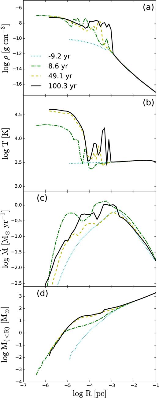
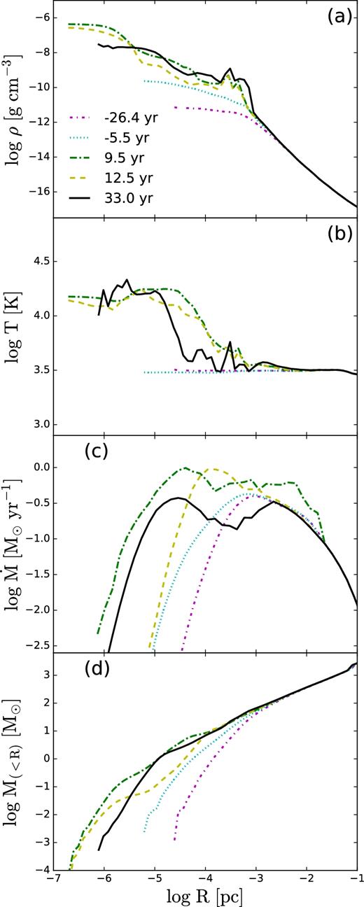
Adiabatic accretion flow. Evolution of (a) gas density, (b) temperature, (c) accretion rate, and (d) mass within spherical radius R, at a few representative times. Negative values correspond to times prior to the establishment of the photosphere.
We have introduced a cut-off in the cooling rate of the flow based on its optical depth (equation 6). Above τ = 1, the cooling rate decreases exponentially. This cut-off mimics the formation of the photosphere, below which the radiation is expected to diffuse rather than free-stream, and the cooling rate is expected to decrease sharply. Very roughly, this condition is fulfilled initially at Rph ∼ 10−6 pc, and this radius expands rapidly to Rph ∼ 10−4–10−3 pc (Fig. 2). The FLD model, described in the next section, behaves similarly.
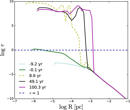
Adiabatic collapse: optical depth profile in the flow at a few representative times. Negative values correspond to times prior to the establishment of the photosphere. The dashed horizontal line delineates the photosphere at τ = 1.
The flow quickly becomes adiabatic interior to this radius, which can be observed by monitoring the cooling rate. Outside Rph, we observe the radiative cooling, Λ, being compensated by compressional heating. Inside Rph, on the other hand, the compressional heating dominates, resulting in a steep rise in temperature.
Fig. 1(a) shows the density profile at four representative times during the collapse. The region where the flow becomes optically thick, Rph, displays a sharp increase in the gas density, which levels off at smaller radii. Note the formation of a central core with R ∼ 10−5 pc at t ∼ 8.6 yr, and a number of density peaks outside the core at later times, which represent the forming fragments, as we discuss below. The temperature profile is closely related to the formation of the core and surrounding fragments (Fig. 1b). The central density and temperature have reached ∼10−7 g cm−3 and 5 × 10⁴ K, respectively. The fragments stand out clearly at the end of the simulation as temperature peaks. By the end, both core radius and the new fragments are situated at larger radii, as Rph has moved out.
The mass accretion rate profile reflects the existence of a disc on scales of 1–10 pc, shown in Fig. 4, which is largely rotationally supported. The inner parts of this disc become unstable and collapse, with accretion rate |${\dot{M}}(R)$|, reaching a maximum and declining further inwards (Fig. 1c). The shape of |${\dot{M}}(R)$| stays largely unchanged with time, except for some variation of the peak position, which shifts back and forth.
As expected and despite formation of a disc at larger radii, the mass accumulates within the central region (Fig. 1d). By t ∼ 100 yr, the amount of gas within the central ∼10−4 pc is ∼40 M⊙, and within 0.1 pc about 2 × 10³ M⊙. The mass within the photospheric radius is ∼100 M⊙ (Fig. 7).
The rotational support on small scales, within Rph, is partial but prominent in the adiabatic flow (Fig. 3b). The flow is rotationally supported, within a factor of 2, at nearly all radii, but gains even more support around ∼10 pc, where it forms a warped disc as discussed above, and around Rph, where it forms a growing geometrically thick disc surrounded by fragments at the later stage (e.g. Fig. 4). The fragments can also be traced in the ρ and T distributions averaged on spherical shells in Figs 1(a) and (b). By t ∼ 100 yr, tangential velocity rises to its maximal value at ∼Rph, then decreases by about a factor of 10, and the radial velocity behaves in the opposite way (Fig. 3a). What is the reason for this decrease in vt and increase in vr at smaller R? We analyse this issue below.
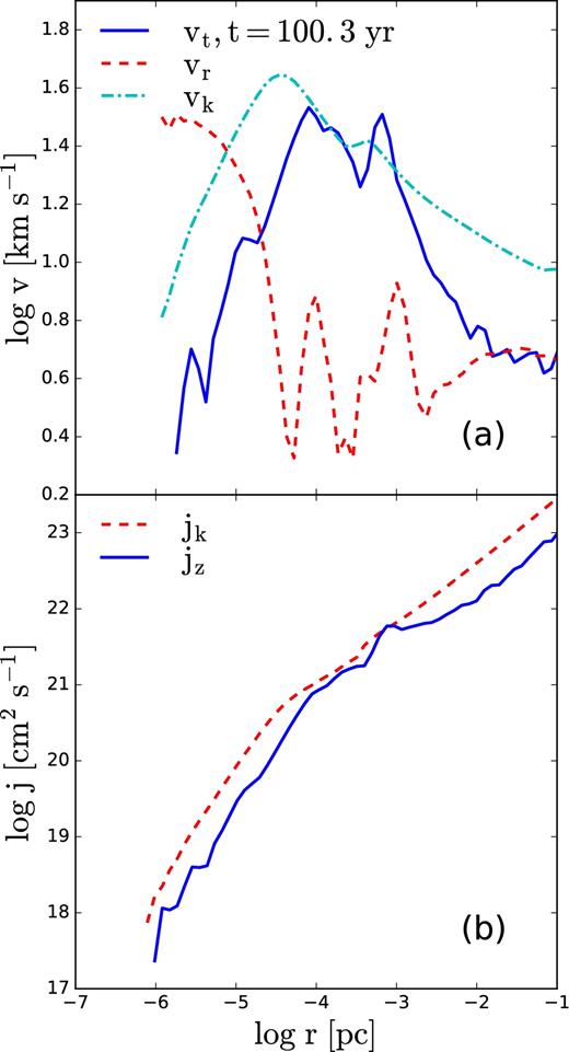
Isolated adiabatic accretion final profiles at t = 100.3 yr: (a) tangential velocity, vt (solid line), radial inflow velocity, vr (dashed line), and circular velocity, vk (dot–dashed line) at cylindrical radius r; (b) specific angular momentum of accreting gas, jz (solid line) and circular specific angular momentum, jk (dashed line) at r.
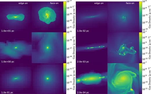
Final projection snapshots of adiabatic collapse on various spatial scales, from 10 pc down to 2 × 10⁻⁴ pc. Shown are two independent directions, roughly corresponding to face-on and edge-on views. Fragmentation is occurring on scales of ∼10−3 pc, somewhat larger than the photospheric scale.
Evolution of the accretion flow on scales of ∼10−3 pc reveals a dominant bar-like mode at early times (e.g. Fig. 5). At a later stage, t ≳ 26 yr, two open spiral arms are driven by this bar-like feature and completely dominate the flow. Fragmentation is seen in projection. Most of the fragments spiral in and merge in the central region.
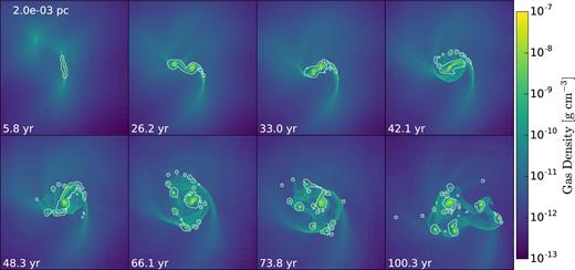
Evolution of adiabatic collapse. Projection snapshots on scale of 2 × 10⁻³ pc. Colour palette is based on logarithmic scale. The white contours represent the photospheric surfaces defined in the text.
Fig. 4 provides more details about the central region of ∼10−4 pc, where one observes a disc, edge-on and face-on, at the end of the run. Fourier analysis of this disc reveals a strong bar-like mode dominating its kinematics, with an amplitude of A2 ∼ 0.46. The m = 1 mode is less important. We have also measured the strength of the gaseous bar using its ellipticity, defined as ε = 1 − b/a, where a and b are the semimajor and semiminor axes (e.g. Martinez-Valpuesta, Shlosman & Heller 2006). The typical value for the late stage is ε ∼ 0.65, which means that a strong bar dominates the potential in this region. This m = 2 mode leads to strong radial flows that explains the radial profiles of tangential and radial velocities.
The distribution of fragment masses is given in Fig. 6. These clumps have been identified by having detached photospheres from the central object, then verified being self-gravitating. The most massive clump corresponds to the central disc, ∼10 M⊙, and the majority of clumps have masses of ∼0.1 M⊙. Their formation is limited to the region dominated by the spiral arms, i.e. within ∼10−4–10−3 pc. In fact, these clumps form along the spiral arms only. The clumps that formed earlier spiral in and are absorbed by the central disc. The number of clumps levels off in time, reaching a steady state.
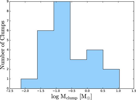
Adiabatic collapse: fragmentation of the flow on scales of ∼10−3 pc (see Fig. 5). The distribution of clump masses is shown.
To understand the reason for fragmentation, we have checked for Toomre instability, characterized by the |$Q=\chi \,c_{\rm s}/\pi G \Sigma$| parameter. Here, χ is the epicyclic frequency, cs is the sound speed, and Σ is the surface density of the discy entity. Based on the properties of the flow, we have calculated Q(r) for t = 27 yr. We find that it dips below unity between 10−4 and 10−3 pc from the centre, i.e. exactly where the clumps are observed to form (e.g. Fig. 5).
However, caution should be exercised here, as the clumps form in the spiral arms, while the underlying disc is ill-defined. An alternative explanation may be related to the Kelvin–Helmholtz (K-H) shear instability (e.g. Chandrasekhar 1961). The open spirals represent shock fronts, and the gas moves through them with a Mach number of |${\mathcal {M}}\sim {\rm few}$|, as can be inferred from Figs 1 and 3. The gas experiences an oblique shock, and the measured pitch angle between the shock front and the gas streamlines is about i ∼ 60°, confirming that the spirals are open and not tightly wound.
We assume that the shock front and the post-shock layer are associated with the spiral arm that perturbs an otherwise axisymmetric background gravitational potential. It is convenient to estimate the value of the gravitational acceleration induced by the spiral arm as a fraction β of the radial potential measured by the centrifugal acceleration, |$v_{\rm t}^2/R,$| where vt is the gas tangential velocity. β ∼ 0.05 is a typical perturbation by a spiral arm in disc galaxies (e.g. Englmaier & Shlosman 2000). To project this acceleration on the direction of the streamlines entering the shock front, we account for the pitch angle i, to obtain |$g\sim \beta v_{\rm t}^2/r {\rm sin}\,i$|. Here, r corresponds to the radius vector extending from the flow centre, i.e. in our case, corresponding to the core centre.
Adopting values from the run, i.e. i ∼ 60°, and b/r ∼ 0.3, we obtain Ri ∼ 0.1. Hence, the flow must be unstable and form clumps along the spiral arms.
Next, we invert the problem, and ask what wavelengths, l/r, are unstable, taking Ri = 0.25 and keeping other values fixed. For K-H shear instability, we obtain l/r < 0.8.
Hence, the K-H shear instability appears as an viable alternative to the Toomre's instability, especially because the fragmentation happens in the spiral arms and the underlying disc is ill-defined. The latter comment refers to the formation of spirals in a sheared flow dominated by a bar-like feature.
The central object, which is supported mainly by rotation and partly by gas pressure gradients, does not show any tendency to fragmentation. This is understandable, because it is geometrically thick and Toomre instability is suppressed with increasing thickness, in contrast to the claim by Becerra et al. (2015).
To demonstrate the mass growth in the central region, we measure the mass evolution contained within three specific radii, i.e. 10−5, 10−4, and 10−3 pc (Fig. 7). For the largest radius, 10−3 pc, the growth is monotonic, and the accumulated mass is about 100 M⊙. The noise increases gradually to smaller radii. The amount of gas within 10−4 pc radius appears to saturate in time, which is explained by the fragmentation. The fragments spiral in more slowly than the smooth accretion flow, and are responsible for the mass accumulation on this scale.
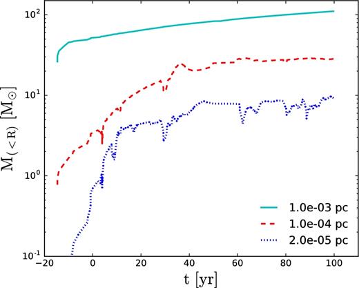
Adiabatic collapse: evolution of the enclosed mass within fixed spherical radii.
To summarize, we clearly observe formation of a central object in the adiabatic accretion flow. This object appears to be supported by both the gas thermal pressure and rotation. The radiation pressure gradients are not important, as the temperature remains relatively low, T < 105 K. Core formation results in a substantially flattened configuration, resembling a geometrically thick disc. It is surrounded by fragments and we lean towards the K-H shear instability explanation for their origin, as opposed to Toomre instability. We return to this issue in the Discussion section.
4 RESULTS: NON-ADIABATIC FLOW
One of the main questions about direct collapse is whether the adiabatic flow approximation used in the literature so far adequately represents evolution. In this sense, the adiabatic run with identical initial conditions serves as a test model of what to expect in the FLD run. The non-adiabatic flow in the isolated model is in many respects similar to that of the adiabatic model but also exhibits some important differences that cannot be ignored. As noted earlier, we consider the FLD flow to be in LTE.
4.1 Deep interior flow: formation and dissolution of the central core
The basic parameters of the FLD flow are shown in Fig. 8. They display the gradual formation of the central object, its photosphere, and its subsequent expansion. The photospheric jump is not as dramatic as in the adiabatic case. The central density is higher at some specific time in the run, then becomes lower. The photosphere forms at 2.037 Myr after the start of the simulation, and t = 0 occurs slightly later in the evolution compared to the adiabatic run, by about 104 yr. The central temperature is lower than in the adiabatic case and remains stable after the formation of the photosphere, ∼1.6 × 10⁴ K. Fragmentation is virtually non-existent, and formation of a few photospheric ‘islands’ is observed, that merge quickly. The FLD flow is filamentary, as in the adiabatic case, with a single dominating filament, as seen in Fig. 9 at early times.
Non-adiabatic accretion flow. Evolution of (from top to bottom) gas density, temperature, accretion rate, and mass within spherical radius R.
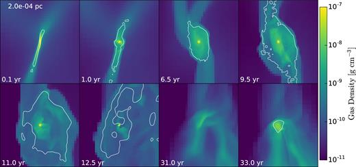
Evolution of non-adiabatic collapse. Projection snapshots on scale of 2 × 10⁻⁴ pc. Colour palette is based on logarithmic scale. The contour line corresponds to the position of the photospheric surface and was calculated using the delimiter λ = 1/3 (Section 2.1). Note that after t ∼ 9.5 yr, the photosphere is expanding because of the extensive outflow from the central core region, then receding. The core dissolves completely by t ∼ 15 yr, and the region becomes marginally optically thin. A new core starts to form at around this time in a slightly different position and reaches ∼1 M⊙ by t ∼ 32 yr. Frames before t = 15 yr have been centred on the existing core, while later frames are centred on the forming new core (see also Figs 11 and 13).
The temperature starts to rise at ∼few × 10−4 pc (Fig. 8b). The rise from T ≲ 3 × 10³ K correlates with a sharp increase in the bound-free opacity in atomic hydrogen. Photoionization quickly becomes the dominant heating mechanism in the gas, surpassing the compressional heating by orders of magnitude. This leads to a sharp increase in the optical depth and to the appearance of the photosphere at τ ∼ 1 that we denote as Rph as in the adiabatic case. This time is taken as t = 0.
The density profile within Rph becomes flatter than R−2 and is rather closer to R−1 (Fig. 8a). Initially, the collapse proceeds deeper than in the adiabatic case, down to ∼10−7 pc, before it is stopped by the gas pressure gradient. The radiation force is about 1 per cent of the gas pressure force at this time (Fig. 12a), then increases to about 10 per cent by t ∼ 9.5 yr, and continues to increase thereafter (Fig. 12b). Rotation is partially important at Rph, but declines sharply at smaller radii (Figs 10 a and b).
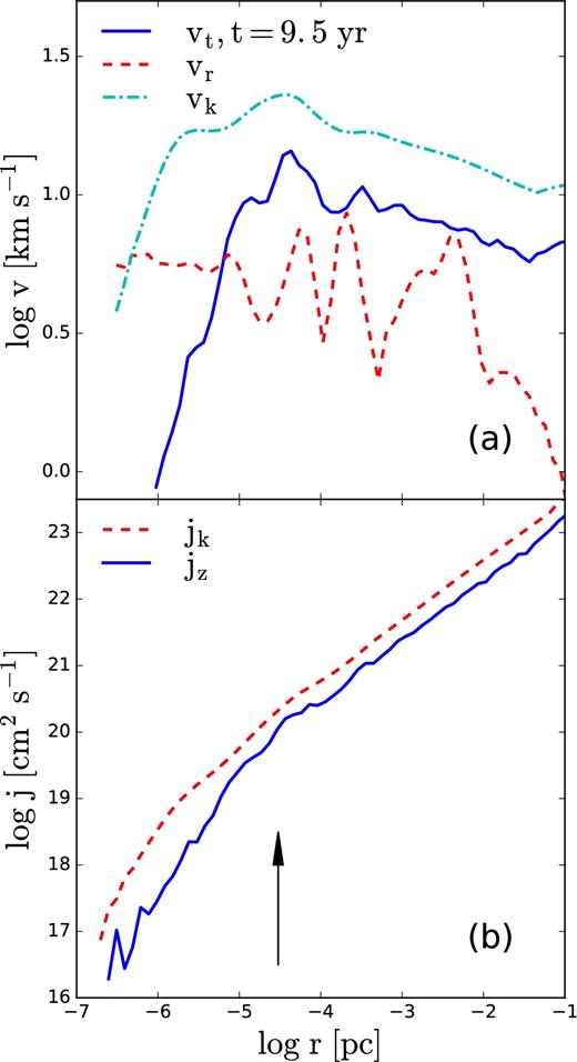
Non-adiabatic accretion flow final profiles of (a) tangential velocity, vt (solid line), radial inflow velocity, vr (dashed line), and circular velocity, vk (dot–dashed line) at cylindrical radius r; (b) specific angular momentum of accreting gas, jz (solid line), and circular specific angular momentum, jk (dashed line) at r. The vertical arrow shows the approximate position of the photosphere.
The evolution starts to diverge from the adiabatic flow at small radii. Within Rph, a core forms and grows to ∼1 M⊙ and size ∼7–8 × 10⁻⁶ pc. Its temperature is lower than the outside gas by a factor of 2, and its density increases. One can observe the associated break in the density profile of Fig. 8(a).
The filamentary inflow develops as the collapse proceeds and extends to the smallest scales achieved in the run. One observes that the inflow is channelled along these filaments, and outside material joins the filaments after experiencing an oblique shock on their surfaces. Additional shocks form in the central region where the two main filaments collide and the flows merge. Velocities abruptly decrease within the innermost shock, pointing to the overall slowdown of the accretion flow, and the start of virialization. Both the thermal pressure gradients in the gas and the rotational support contribute to this dramatic slowdown and essentially terminate the accretion flow.
To understand the prevailing structure on these scales, refer to Fig. 11, which provides views of the region on scales R ∼ 2 × 10⁻⁴ pc (top frames) and R ∼ 2 × 10⁻⁵ pc (bottom frames) at t ∼ 9.5 yr. Density, temperature, and flow pattern are shown. On smaller scales, one observes a small dense core that is nearly round, confirming the unimportance of rotation. This core is surrounded by a hotter and much less dense, expanding envelope. This is more visible on the larger scale, where a system of nested shocks is created by this expansion against the collapsing gas within the main filament. The overall configuration is that of a small dense core surrounded by expanding hot bubbles driven mostly by gas pressure and a non-negligible contribution from radiation pressure gradients.
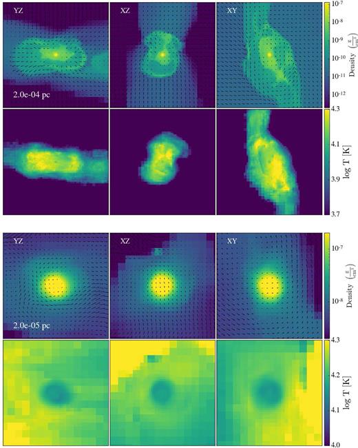
Non-adiabatic accretion final projection snapshots from three independent directions on scales of 2 × 10⁻⁴ pc (top) and 10−5 pc (bottom) at t ∼ 9.5 yr (see corresponding Fig. 13 a frame at this time). On each scale, we show the density and velocity fields projections (top) and the temperature (bottom). Note the developing anisotropic outflow from the central core along the filament and the associated expanding bubble driven by this outflow. The shape of the core is clearly outlined by the large density contrast with the environment. Its interior temperature is slightly lower than that of the surrounding gas.
An interesting feature is that the core is colder than the expanding bubbles above the photosphere, as the temperature map conveys. This, in tandem with lower density above Rph, allows the radiation force to be more important at and above the photosphere. It also explains the driving forces behind the outflows.
By t ∼ 12.5 yr, the radiation force becomes comparable to the gas thermal pressure gradients (Fig. 12c), dramatically increasing the mass outflow rate. Fig. 9 shows the evolution of the photosphere, which by this time becomes very extended, well outside the colder core. The core mass decreases sharply, as it is ‘eaten away’ by the outflow.
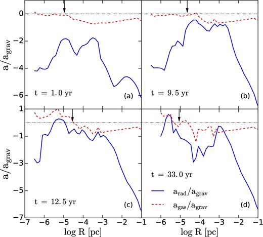
Dominant accelerations in the non-adiabatic accretion flow: thermal pressure gradient (dashed red line) and radiation pressure gradient (solid blue line) normalized by gravitational acceleration of the enclosed mass at t ∼ 1, 6.5, 12.5, and 32.7 yr. The dotted line is drawn to delineate the ratio of unity. The vertical arrows show the approximate position of the photosphere.
This process starts at around t ∼ 8 yr, when a strong outflow develops and extends up to and above ∼10−4 pc, as shown in Fig. 11 at t = 9.5 yr. By t ∼ 15 yr, the core dissolves completely and the photosphere disappears.
We have checked the existence of the photosphere using two independent methods outlined in Section 2.1, by calculating the 3D shape of the photosphere using (1) the values of the limiter, λ = 1/3, as a trace of the optically thick region, and (2) the optical depth by integrating along about 4900 independent rays to τ = 1. Both methods produces similarly shaped contours, with the latter contour lying at slightly larger radii. The result of the first method is displayed in Fig. 9. We have also introduced a spherically averaged photospheric radius Rph, which we use in the associated discussion. Fig. 13 displays the photospheric radius calculated using this method.
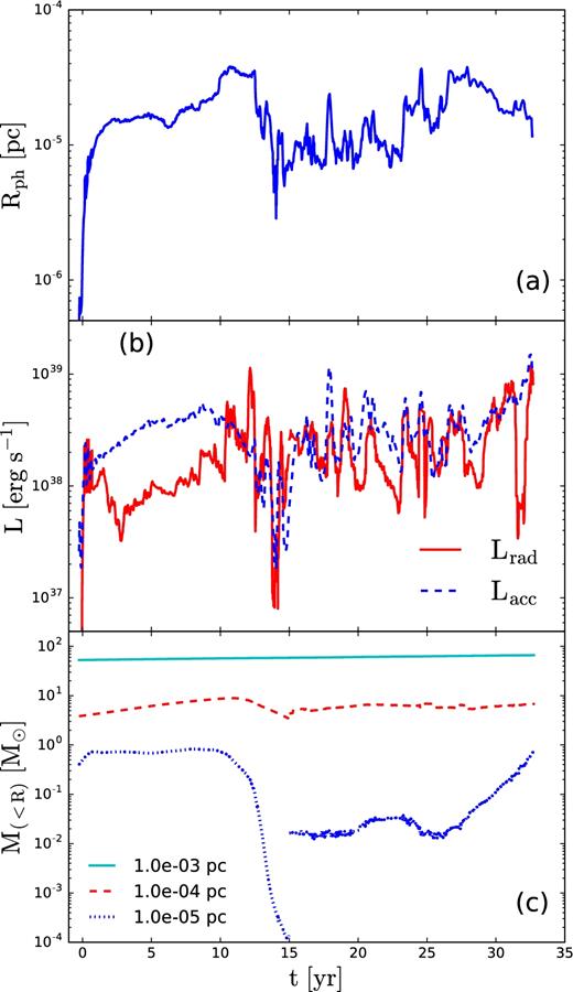
(a) Evolution of the spherically averaged photospheric radius, Rph, of the first core (t ≲ 15 yr) and the second core thereafter. (b) Evolution of radiation luminosity, Lrad, and accretion (mechanical) luminosity, Lacc, in the non-adiabatic model based on the photospheric radius shown. (c) Evolution of the enclosed mass within a fixed radius. The discontinuity in the dotted line reflects the dissolution of the first core at t ∼ 15 yr and the subsequent growth of a nearby core.
A second core forms nearby, separated by ∼3 × 10⁻⁴ pc from the first core, and has an initial mass of ∼0.01 M⊙, but does not show any growth for a few years. It starts to grow rapidly after t ∼ 25 yr. The new photosphere appears at t ∼ 30 yr and the core mass reaches ∼1 M⊙ in about 5 yr, exhibiting a growth rate of ∼0.2 M⊙ yr−1 (Fig. 9). By the end of the run, the central density of the second core, ∼3 × 10⁻⁸ g cm−3, had not yet reached the peak density of the first core, but it is still increasing with time (Fig. 8a).
Because of the perturbing action of the mass inflow, variations in ρ and T, and the dependence of opacity on these parameters, the position of the photosphere, Rph, is erratic and it is far from having spherical symmetry. This is similar to the adiabatic run. Fig. 13 (top frame) provides the evolution of the spherically averaged Rph with time. The photosphere for the FLD run is close to that of the adiabatic model initially, before the outflow develops. Within the photosphere, however, the evolution differs significantly, e.g. in the importance of radiation pressure and rotation, and in the overall outcome.
The central objects appear well resolved during the simulations. Their masses, ∼1 M⊙, are well above the local cell mass of ∼10−6 M⊙. The resolution limit is ∼3 × 10⁻⁷ pc.
For an isolated virialized system, the virial ratio is X = 2Ekin/|W| = 1, where Ekin is the total kinetic energy within the object, including the bulk and random motions, the radiation pressure is still not important, and W is its gravitational energy. Since cores obtained in our simulations are accreting at a high rate kinetic and thermal energies as well, and experience mass loss, and we must also include the relevant surface term in calculating X (e.g. Landau & Lifshitz 1980).
For each of the cores formed, we calculate their virial ratios, X(t) ≡ (2Ekin − 3PphV)/|W|, assuming their spherical symmetry, as a function of time. X is calculated assuming the boundary of the object's ‘surface’ lies at Rph ∼ 10−5 pc. Here, Pph is the total pressure, i.e. the thermal and kinetic energies of the gas at Rph, and V is the volume of the object. We account for the gas thermal energy in the accretion term because the radial velocity of the flow is of the order of its sound speed. 3PphV corresponds to the surface term in the Virial Theorem.
The contribution of the surface term, which consists of the flow of the bulk kinetic and thermal energy of the gas should reduce the X value below unity. The sign of Pph term depends on the relative importance of outflow and accretion averaged over the surface. It could be positive or negative, so the surface term could increase or decrease X. Indeed, this is what is observed – X varies below unity initially, which delineates the unsteady contribution of the mass accretion flux. For the first core, X becomes larger than unity thereafter and steadily increases, reflecting the dissolution of the core.
4.2 The photosphere: radiation luminosity
Accreting mass flux carries a substantial kinetic energy because of the large |$\dot{M}_{\rm acc}$|. What is the efficiency of converting this mechanical energy into radiation?
The kinetic energy of the accretion flux, measured at Rph, varies by about one decade within Lacc ∼ 5 × 1037–5 × 1038 erg s−1, and is of the order of the Eddington luminosity, ∼1038 erg s−1, for electron scattering opacity (Fig. 13b). Note that the Rosseland mean opacity we use is of the order of the electron scattering opacity for these temperature and density values. The range in Lacc is determined by motion of the photospheric radius and temporal variation of the mass accretion rate and radial inflow velocity (Figs 8 and 10). The largest dip in Lacc is strongly correlated with the dissolution of the first core, and the associated mass outflow in the region close to Rph (Fig. 13b). This process slows down the mass influx within the central ∼10−4 pc. The influx is restored 10 yr later, but it becomes much more noisy.
The evolution of radiation luminosity, Lrad, at some periods correlates with Lacc, and in other periods it anticorrelates (Fig. 13b). During the monotonic growth periods of both cores, it clearly correlates. This behaviour is disrupted by the powerful outflow that is associated with the dissolution of the core.
We have performed a Fourier analysis of the L and Lacc curves in Fig. 13(b). The power spectrum of Lacc variability peaks around the characteristic time-scale of ∼10 yr. It corresponds to the accretion time-scale for a typical distance of few × 10−5 pc and the observed inflow velocities of ∼3 km s−1. However, this time-scale should be taken with caution, as the simulation has been run only for about 40 yr, and so this time-scale can be subject to temporal aliasing.
Additional and more rapid variability in Lrad is present at all times, but its amplitude increases following dissolution of the first core. The power spectrum also has a low peak at the characteristic time-scale of ∼0.12 yr. Typically, Lrad correlates with the accretion rate, but in some cases the response in Lrad is either delayed or non-existent. During peaks of this variability, the radiation luminosity can exceed the accretion power by a factor of a few, and Lrad can exceed ∼1039 erg s−1. Clearly, energy can be stored within the photosphere, in either mechanical or radiative form, and released suddenly.
5 DISCUSSION
We have followed direct baryonic collapse within isolated DM haloes. Inclusion of radiative transfer and the associated physics have allowed us to reach spatial scales of ∼0.01 au, or ∼10−7 pc, for the first time in a meaningful way. The radiative transfer has been performed in the FLD approximation and LTE has been assumed for the optically thick collapsing region.
For comparison, we have run an adiabatic model, where the cooling rate has been exponentially damped below the τ = 1 surface. We have tested the code by running a number of models describing the evolution of a shock induced by a photoionization source at the centre of a hydrogen cloud. These models have been executed with FLD, and with and without LTE, as detailed in the Appendix. Moreover, they have been compared to published models in the literature, where analytical fits have been provided.
We find that the collapse proceeds in a filamentary way and remains nearly isothermal in the outer part, down to ∼10−5 pc from the centre. The gas is channelled along the filaments, with oblique shocks formed by the material when joining the filaments. Inside the optically thick region, a central object forms in response to the converging flow and reaches a mass of ∼1 M⊙. Growing radiation and thermal pressure gradients within the object exceed the gravitational acceleration, triggering a strong outflow, originating close to the photospheric radius. The outflow has a bursting behaviour and drives expanding nested hot bubbles. The central core that forms deeper inside the photosphere is close to dynamical equilibrium, but as the outflow ‘eats up’ the core from outside in, the core dissolves completely and the optical depth of the central ∼10−4 pc hovers around unity. Another core forms in its vicinity and grows rapidly, reaching ∼1 M⊙. The region inside the photosphere and its structure are well resolved in our simulations.
The FLD model leads to the formation of an object that is supported mostly by gas thermal pressure, and with some degree of rotation in the outer sub-photospheric layers. While the photosphere has a complex elongated shape, the core of the object is quasi-spherical. This is in a stark contrast with the adiabatic model, where the central object is discy and of a convex shape, and is dominated by rotation.
The photosphere forms somewhat later, by ∼104 yr, in the FLD run – a consequence of additional radiation force operating in the region. (Note that initial conditions are identical for both runs.) If one compares both runs at t ∼ 33 yr, when the FLD model has been terminated, substantial differences point to diverging evolution.
Specifically, the adiabatic model has a higher temperature in the central region, by a factor of 3, due to inability of the optically thick flow to cool down. And the central mass accumulation is higher than in the FLD case, where a combination of radiation force and thermal gas pressure gradients has driven a massive outflow. These factors leads to a different radial profile of the specific angular momentum in the gas. In particular, the ratio of the angular momentum to the maximally allowed value is about unity in the adiabatic case – a clear sign of a rotational support – whereas this ratio is smaller by a factor of a few in the FLD run. Consequently, the kinematics of the adiabatic flow differs from that of the FLD runs. Lastly, the adiabatic model shows fragmentation on scales of ∼10−4–10−3 pc, while no fragmentation has been observed in the FLD runs.
This means that the central object will be identified in the simulation at around this mass and is expected to be in very rough equilibrium only, with a mixture of thermal and radiation pressure gradient, gravity, rotation, and internal turbulence. The reason why much smaller objects cannot be identified lies in the fact that smaller objects will be buffered substantially by the inflow, the position of their centre of mass will be destabilized, and their shape will be completely arbitrary. This is not a semantic difficulty, but rather a condition for the object to separate itself from the dynamic inflow.
The next question to be answered is related to the difference between the adiabatic and FLD models. In a simplistic argument, one can make a case that the adiabatic equation of state adequately describes the behaviour of the gas when an optical depth exceeds unity and the cooling declines exponentially. Initial conditions for the adiabatic and FLD runs are identical and cannot explain the different outcome. Besides, for gas evolution, initial conditions play secondary role, as the system quickly forgets them. What is the source of the diverging evolution of these models?
The adiabatic equation of state presumes that the cooling is completely unimportant, and individual parcels of the gas do not exchange energy even in the presence of temperature gradients. This requirement may be too restrictive. In a system that is not virialized, and basically consists of streamers originating from strongly anisotropic inflow and is loosely bound, large temperature gradients build up. This can be seen from Fig. 14(b), which shows the dispersion in the gas temperature around the mean, given by Fig. 8. The meaning of this is that the photons leak along large temperature gradients. The non-spherical shape of the photosphere assists in this process. This effect is absent in the adiabatic flow.
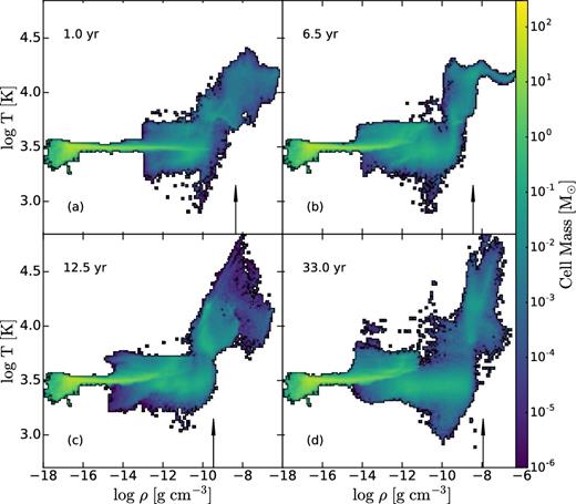
Evolution of the non-adiabatic accretion flow with FLD: temperature versus gas density, at t ∼ 1, 6.5, 12.5, and 32.7 yr. The colour palette shows the total mass of all grid cells with the same density and temperature. The vertical arrows show the approximate position of the photosphere.
Next, we discuss the central mass accumulation over the simulation time. Even over the 35 yr run time since the formation of the photosphere in the FLD flow, about 10 M⊙ are expected to be added at the photospheric radius. Figs 8(d) and 13 do not show such evolution on the scale of Rph. On the other hand, Fig. 8(c) confirms that the high accretion rate peak moves to larger radii, outside Rph. The explanation lies with the evolution in the presence of a strong outflow that acts against the mass accumulation inside the photosphere. Instead the gas accumulates inside R ∼ 10−3 pc, as shown in Fig. 13(a), which displays the amount of material inside this radius.
Models that quantify the amount of gas in the central region, and that ignore the feedback, show the fast assembly of a massive object there (Shlosman et al. 2016). The current FLD run argues against this conception. What does appear as important is that radiation feedback has an effective distance beyond which it can be ignored. The FLD run puts this radius at ∼10−3 pc, where by the end of the simulation about 100 M⊙ has been accumulated. This is about 200 au – the size of the Solar system. Within the typical star formation framework, this is probably nothing outstanding, when, e.g. an O star forms. What is different here is the rate of accretion that exceeds that of the star formation by an order of magnitude. Thus, one cannot argue that radiation feedback will terminate accretion on the ‘protostar’ and its growth.
The present state of the central region in the FLD run can be characterized as in a ‘splash’ stage. The gas accretion flow converges in the centre and gravity is not capable of confining the resulting random motions to within the photosphere. The radiation force at the photospheric radius is close to the Eddington limit given the amount of mass in the region and the radiative luminosity (Figs 8 d and 13b). Overall, such conditions are not encountered in the star formation process, where both mass accretion rates and inflow velocities are dramatically lower, implying that the virialization process is much less violent.
Some hints for the further evolution of the system can be inferred. The radiation-driven outflow is confined to within ∼10−3 pc, where the kinetic energy of the accretion can contain the kinetic energy of the outflow. Once the outflow is stopped, the gas will have no pressure or rotational support and must resume the collapse. We anticipate that additional outflow stages will follow but with progressively smaller amplitudes. But this does not mean that the system will virialize easily.
A separate question is whether the above evolution leads to the formation of a single massive object, e.g. an SMS, which will virialize and whose central temperature will exceed few × 106 K, enabling the proton–proton chain of thermonuclear reactions, and further stabilizing the SMS. Our FLD runs, which appear to be more realistic than the adiabatic ones, have less rotational support in the centre, yet it is not negligible. Continuing accretion will bring fresh material with increasing angular momentum. The reason for this is that low-J gas is naturally accreted first, and the subsequent accretion will increase its J. Because of a large accretion rate, this can lead to a spin-up of the object, non-axisymmetric instabilities, and a resumption of the central runaway, similarly to the scenario that happened at ∼1 pc in the earlier stage.
The difference in the evolution between the adiabatic and FLD models emphasizes the importance of the proper treatment of radiative transfer in the optically thick phase of gravitational collapse. This requires a seven-dimensional phase space to obtain the radiative intensity, which is impossible to achieve at present even numerically. Both Monte Carlo and direct discretization methods require too many computational resources. Limiting calculations to radiative flux and energy allows one to take the angular moments of the equations of radiation hydrodynamics. Examples of such low-order closures are FLD, discussed in Section 2.1, and the M1 closure (e.g. Levermore 1984; Janka et al. 1992). Their deficiency lies in an inadequate treatment of the Eddington tensor, which is symmetrized about the direction of the flux. In certain cases, this crude approximation can fail (e.g. Jiang, Stone & Davis 2012).
Both FLD and M1 can be applied in the optically thin and thick regions. Potentially, the FLD method can lead to errors, as it has difficulty to capturing the shadow formed even by one beam (e.g. Gonzalez, Audit & Huynh 2007), while the M1 method cannot propagate two beams correctly, having difficulty following the radiation field in complex geometries (e.g. McKinney et al. 2014).
The weak point of both FLD and M1 algorithms – their difficulty in handling the transition between optically thick and thin regions – can be supplemented by the ray-tracing method. This approach was implemented in the PLUTO grid code for a spherical polar grid (e.g. Kuiper et al. 2010). As ray-tracing is a solution to the radiative transfer equations, FLD is an approximation, there is a clear advantage in combining both methods (e.g. Klassen et al. 2014). This means, using direct ray-tracing in optically thin regions, where scattering can be ignored, while implementing FLD in optically thick regions, where diffusion dominates.
An algorithm that is based on the direct solution of the radiative transfer equations and that does not invoke a diffusion approximation has been proposed for the MHD code Athena (Jiang et al. 2012). The hierarchy of moment equations has been closed using a variable Eddington tensor, whose components have been calculated using the method of short characteristics, still computationally expensive. Further improvements must follow along these lines.
6 CONCLUSIONS
We have simulated the radiative transfer in gravitationally collapsing primordial gas within isolated DM haloes, so-called direct collapse. Models in the cosmological framework are dealt with in an associated publication (Ardaneh et al. 2018). We focus on the optically thick part of the collapse, initially at radii below ∼10−6 pc, 0.1 au, where the photosphere of the central object has formed. The radiative transfer was performed in the flux-limited diffusion (FLD) approximation, using a modified version of the Enzo-2.4 AMR code, and LTE conditions were assumed. For comparison, we have run adiabatic models, and additional testing of the FLD module is shown in the Appendix.
We find that the collapse is dominated by filamentary structure modified by rotation, down to the photospheric scale. The central object that forms within the photospheric radius grows to ∼1 M⊙, and is supported mainly by thermal gas pressure gradients with the addition of rotation. The evolution of this object is heavily perturbed by the penetrating accretion flow that peaked at ∼0.5 M⊙ yr−1, growing temperature and increasing radiation pressure. The photospheric luminosity is close to the Eddington limit. This leads to the development of an anisotropic outflow driven by radiation force, which disrupts the central object and dissolves it, driving a series of expanding hot bubbles interacting with the accretion flow.
The dissolution of the core leads to the formation of another core nearby, which grows efficiently and shortly reaches ∼1 M⊙. With the formation of this object the central temperature starts to grow, sharply decreasing the time-step. At this point, the enclosed mass within the central 10−3 pc is about 100 M⊙, with about 3 × 10³ M⊙ within the central 0.1 pc.
This mass accumulation agrees with that of the adiabatic run, but its kinematics is substantially different. The adiabatic run forms a geometrically thick disc, supported mainly by rotation with an admixture of thermal gas pressure. Outside this disc, a number of fragments form that show a tendency to merge with the central convex-shaped disc. This fragmentation is observed on scales between ∼10−4 and 10−3 pc, and temporarily disrupts the growth of the central object. This object is in contrast with quasi-spherical shapes of the forming cores in the FLD case.
In both cases, the photospheric shapes are very irregular, which allows the radiation to diffuse out of the central region. This explains the major difference between the adiabatic and the FLD runs, and reveals the inapplicability of the adiabatic approximation to the growth of the central core in direct collapse.
We find that the typical radiation luminosity from the photosphere of each of the cores formed lies in the range of ∼few × 1037 − few × 1038 erg s−1 over much of the run time. This is of order the Eddington luminosity for such an object. Fourier analysis shows that this luminosity varies on two characteristic time-scales: a long one, which is associated with the variable accretion time-scale, and ∼0.1 yr, which originates in the radiative diffusion time-scale within the photosphere. The latter variability is characterized by a large amplitude that exceeds 1039 erg s−1.
This study reveals that models accounting for radiative transfer in the collapsing gas display a different evolution than models with an adiabatic equation of state, at least during early stages of core formation. The main reason for these differences is that the radiation is capable of diffusing out due to the anisotropy in density and temperature, and the resulting decrease in opacity in various directions. This effect vanishes in the 1D case and requires a multi-dimensional treatment. The underlying gas dynamics changes as a result, leading to massive outflows from forming cores. It modifies the angular momentum transfer, and the flow avoids fragmentation in the optically thick regime, which prevails in the adiabatic case.
ACKNOWLEDGEMENTS
We thank the Enzo and yt support team for help. All analysis has been conducted using yt (Turk et al. 2011), http://yt-project.org/. We thank Daniel Reynolds for help with the FLD solver and Kazuyuki Omukai for providing the updated opacities for a comparison. Discussions with Pengfei Chen, Michael Norman, Kazuyuki Omukai, Daniel Reynolds, and Kengo Tomida are gratefully acknowledged. This work has been partially supported by the Hubble Theory grant HST-AR-14584 and JSPS KAKENHI grant 16H02163 (to I.S.). I.S. and K.N. are grateful for a generous support from the International Joint Research Promotion Program at Osaka University. J.H.W. acknowledges support from NSF grant AST-1614333, Hubble Theory grants HST-AR-13895 and HST-AR-14326, and NASA grant NNX-17AG23G. M.B. acknowledges NASA ATP grants NNX14AB37G and NNX17AK55G and NSF grant AST-1411879. The STScI is operated by the AURA, Inc., under NASA contract NAS5-26555. Numerical simulations have been performed on XC30 at the Center for Computational Astrophysics, National Astronomical Observatory of Japan, on the KDK computer system at Research Institute for Sustainable Humanosphere, Kyoto University, on VCC at the Cybermedia Center at Osaka University, as well as on the DLX Cluster of the University of Kentucky.
REFERENCES
APPENDIX A: EXPANSION OF AN H ii REGION AROUND A POINT SOURCE OF RADIATION: THE ROLE OF THE RADIATION FORCE
To study the role of the radiation force, we set up a cubic box and place a point source L = 106L⊙ at the centre of the box. The simulation box is resolved with 1283 cells. The point source emits ionizing photons in the energy band 13.6–24.6 eV into an initially uniform neutral pure hydrogen gas at a temperature of T0 = 103 K. The tests are performed for three different initial gas number densities, namely 105, 107, and |$10^{9} {\ \rm cm^{-3}}$|. For each number density, the simulation is performed with and without the radiation force, while the photoionization heating is present in both cases. The box size and run time for each test are summarized in the Table A1. For these tests, we assume non-LTE conditions, which means that we solve for the H-chemistry, do not assume Planckian emissivity, and calculate emission versus absorption in this energy bin.
Simulations setup for expanding H ii region.
| Parameter | Test I | Test II | Test III |
|---|---|---|---|
| L | 106L⊙ | 106L⊙ | 106L⊙ |
| nH (cm−3) | 105 | 107 | 109 |
| Lbox (pc) | 2 | 0.2 | 0.02 |
| trun (Myr) | 1.2 × 10⁻² | 2.1 × 10⁻³ | 2.7 × 10⁻⁴ |
| Parameter | Test I | Test II | Test III |
|---|---|---|---|
| L | 106L⊙ | 106L⊙ | 106L⊙ |
| nH (cm−3) | 105 | 107 | 109 |
| Lbox (pc) | 2 | 0.2 | 0.02 |
| trun (Myr) | 1.2 × 10⁻² | 2.1 × 10⁻³ | 2.7 × 10⁻⁴ |
Fig. A1 shows the H ii front expansion driven by a direct momentum absorption from the ionizing source (equation A1), or as a result of the photoionization heating only (equation A2). It clearly shows that radiation force has a trivial contribution at the lowest density 105 cm−3, and the expansion is controlled by photoionization heating (equation A2). As the density increases, at first, the contribution of radiation force in the expansion exceeds the photoionization heating (see the green line in Fig. A1 for time ≤104 yr), and the photoionization heating dominates the process afterwards (see Fig. A1 for time ≥105 yr).
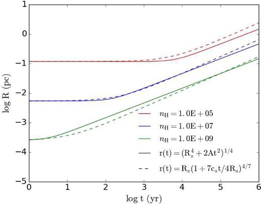
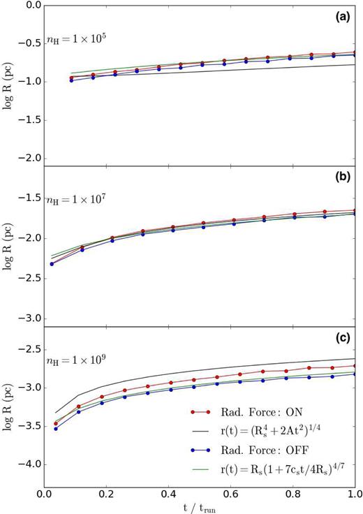
For the performed tests, the H ii front radius is compared with equation (A1), for the cases when the radiation force has the dominant effect, and compared with equation (A2), when the effect of photoionization heating is dominant. Shown in Fig. A2 is the radial evolution of the expanding H ii region for different densities. The radius is estimated to be located where the neutral fraction xH I = 0.5. As discussed before, the radiation force has a negligible effect for the case of nH = 105 cm−3. Therefore, the H ii front radius is mainly determined by the photoionization, and the simulations with and without the radiation force yield quite similar results (e.g. see panel a). As the density increases, the radiation force becomes more important. For density nH = 107 cm−3, panel b shows that the radiation force has small additional contribution to the H ii front expansion, which agrees with the analytical solution. A more significant effect of the radiation force was found for a density of nH = 109 cm−3 (panel c), where the expanding H ii region is governed by the radiation force (see the red circles), and its front radius is well approximated by equation (A1), black line. The correspondence between the analytical and numerical solutions is very good.
Radius of the expanding H ii region versus time for the numerical simulation including the radiation force (red circle) and without radiation force (blue circle). The analytical evolution of the radius due to the radiation force (black dashed line, equation A1) and due to the photoionization heating (green dashed line, equation A2) are also provided.
Shown in Fig. A3 are radial profiles of (a) the gas density, (b) the neutral fraction, (c) the temperature, and (d) the ratio of radiation-to-thermal pressure for an initial number density of 109 cm−3. The profiles of density and neutral fraction in each figure (panels a and b) clearly demonstrate the expansion of the H ii region. For this case, the radiation force is dominant. The gas density and hence the neutral fraction substantially decrease in the H ii region (by about two orders of magnitude), and the ratio of radiation-to-thermal pressure increases by almost two orders of magnitude. Therefore, the resulting expansion of the bubble is mainly driven by a direct radiation force.
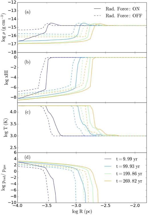
Radial profiles of (a) the gas density, (b) the neutral fraction, (c) the temperature, and (d) the ratio of the radiation pressure to gas pressure given at different times for the initial hydrogen number density is nH = 109 cm−3. Runs with only photoionization heating are represented by dashed curves, while runs that include a radiation force from the ionizing photons are given by solid curves.
There are two important issues to point out. First, for the case of a dominant radiation pressure, the bubble expansion will be stalled at a radius R1, where the outwards radiation pressure from the point source is equal to the thermal pressure from outside the bubble, |$L/4\pi R_1^2 c=n_{\rm H} k_{\rm B}T_0$|. Secondly, in regards to dominant photoionization heating, the expansion stops when nbTb = nHT0, where nb and Tb are gas density and temperature in the bubble. The radius of the bubble in this case can be estimated from |$\dot{N}_{\rm \gamma }=4/3\pi R_2^3\alpha _{\rm B}n_{\rm b}^2$|. Within this radius, the ionizing luminosity of the point source provides an equal rate of photoionizations to the recombination rate within the bubble.
As one can see, the terminal radius of the bubble cannot be determined using equation (A1) and equation (A2) and happens to lie well outside our calculation domain. Rosdahl & Teyssier (2015) presented the expanding H ii region runs with the RAMSES–RT code. In these runs, the maximal bubble radii have been reached and agreed well with R1 and R2 for the dominant radiation pressure and photoionization heating, respectively.
