


Abstract
We calculate axisymmetric magnetic modes of a neutron star possessing a mixed poloidal and toroidal magnetic field, where the toroidal field is assumed to be proportional to a dimensionless parameter ζ0. Here, we assume an isentropic structure for the neutron star and consider no effects of rotation. Ignoring the equilibrium deformation due to the magnetic field, we employ a polytrope of the index n = 1 as the background model for our modal analyses. For the mixed poloidal and toroidal magnetic field with |$\zeta _0\not=0$|, axisymmetric spheroidal and toroidal modes are coupled. We compute axisymmetric spheroidal and toroidal magnetic modes as a function of the parameter ζ0 from 0 to ∼1 for the surface field strengths BS = 1014 G and 1015 G. We find that the frequency ω of the magnetic modes decreases with increasing ζ0. We also find that the frequency of the spheroidal magnetic modes is almost exactly proportional to BS for ζ0 ≲ 1 but that this proportionality holds only when ζ0 ≪ 1 for the toroidal magnetic modes. The wave patterns of the spheroidal magnetic modes and toroidal magnetic modes are not strongly affected by the coupling so long as ζ0 ≲ 1. We find no unstable modes having ω2 < 0.
1 INTRODUCTION
Quasi-periodic-oscillations (QPOs) found in the tail of the giant X/γ-ray flares of SGR 1806-204 (Israel et al. 2005) and SGR 1900+14 (e.g. Strohmayer & Watts 2005, 2006; Watts & Strohmayer 2006) have brought about an intense interest in the oscillations of magnetars, i.e. strongly magnetized neutron stars (e.g. Woods & Thompson 2006; Mereghetti 2008). Because of the suggestion made by Duncan (1998) before the detection of the magnetar QPOs, the crustal torsional oscillations of magnetized neutron stars were first investigated as a candidate for the QPOs (e.g. Glampedakis, Samuelsson & Andersson 2006). However, motivated by the suggestion that the torsional modes in the solid crust will be quickly damped by frequency resonance with Alfvén continuum in the fluid core (Levin 2006, 2007), many researches carried out MHD simulations that follow time evolution of small amplitude and global toroidal perturbations to investigate modal properties of magnetars (e.g. Sotani, Colaiuda & Kokkotas 2008; Cerdá-Durán, Stergioulas & Font 2009; Colaiuda & Kokkotas 2011; Gabler et al. 2011, 2012). For example, Gabler et al. (2011, 2012) showed that because of resonant damping associated with Alfvén continuum in the fluid core the crustal modes cannot survive long enough to explain the observed QPOs. They also suggested that Alfvén modes, instead of crustal modes, could be responsible for the QPOs if the field strength is higher than ∼1015 G since the damping time-scales of Alfvén modes are much longer than those of the crustal torsional modes suffering resonant damping with Alfvén continuum.
These early studies of the oscillations of magnetars are mainly concerned with axisymmetric toroidal modes of the stars, expecting that toroidal modes are probably easily excited to observable amplitudes since they produce no density perturbations. For axisymmetric oscillations of magnetized stars, spheroidal and toroidal components of the perturbed velocity fields are decoupled and can be treated separately for a purely poloidal or toroidal magnetic field configuration for non-rotating stars. This property remains true even for general relativistic treatment. For non-axisymmetric oscillations of magnetized stars, however, the toroidal velocity component is coupled with the spheroidal one which accompanies the density and pressure perturbations, even if we assume a pure poloidal or toroidal magnetic field for non-rotating stars.
Lander, Jones & Passamonti (2010) and Passamonti & Lander (2013) discussed, using MHD simulations, such non-axisymmetric oscillation modes of magnetized stars assuming a purely toroidal magnetic field. For rotating magnetized stars, the modal property will be more complicated because the spheroidal (polar) and toroidal (axial) components of the perturbed velocity fields are coupled and rotational modes such as inertial modes and r-modes come in as additional classes of oscillation modes. Lander & Jones (2011) calculated non-axisymmetric oscillations of magnetized rotating stars for a purely poloidal magnetic field. They obtained polar-led Alfvén modes which reduce to inertial modes in the limit of |${\cal M}/{\cal T}\rightarrow 0$|, where |$\cal M$| and |$\cal T$| are magnetic and rotation energies of the star. Lander & Jones (2011) also suggested that the axial-led Alfvén modes could be unstable.
For mixed poloidal and toroidal magnetic fields, coupled spheroidal and toroidal velocity fields have to be considered to describe global oscillations of the magnetized stars, even for axisymmetric oscillations. Note that assuming mixed poloidal and toroidal fields for the modal analyses is favorable from a magnetic stability point of view since pure poloidal and pure toroidal magnetic field configurations are known to be unstable (e.g. Tayler 1973; Markey & Tayler 1973, 1974; Yoshida & Eriguchi 2006; Yoshida, Yoshida & Eriguchi 2006; Akgün et al. 2013; Herbrik & Kokkotas 2017). Colaiuda & Kokkotas (2012) calculated axisymmetric toroidal oscillations of neutron stars for such a mixed field configuration. They found that the oscillation spectra of the toroidal modes in the core are significantly modified, losing their continuum character, by introducing a toroidal field component and that the crustal torsional modes now become long-living oscillations. This finding may be similar to the finding by van Hoven & Levin (2011, 2012), who suggested the existence of discrete modes in the gaps between frequency continua, using a spectral method. Using MHD simulations, Gabler et al. (2013) discussed axisymmetric toroidal modes of magnetized stars assuming various magnetic field configurations, but they did not find any long-lived discrete crustal modes in the gap between Alfvén continua in the core.
In this paper, instead of MHD simulations of small amplitude oscillations, we carry out normal mode analyses of a magnetized neutron star which possesses a mixed poloidal and toroidal magnetic field for axisymmetric oscillations. In normal mode analysis, the time dependence of the oscillations is given by the factor eiωt and we look for the oscillation frequency ω as an eigenvalue to the set of linear differential equations that govern the oscillations. This paper will belong to a series of studies of normal modes of magnetized neutron stars (Lee 2007, 2008, 2010, 2018; Asai & Lee 2014; Asai, Lee & Yoshida 2015, 2016). The frequency ranges of magnetic modes obtained by normal mode calculations are similar to those by MHD simulations. However, the results obtained by normal mode analyses and MHD simulations are not necessarily fully consistent with each other. For example, although Lee (2008) and Asai & Lee (2014) obtained discrete toroidal magnetic normal modes of neutron stars for a poloidal magnetic field, MHD simulations for axisymmetric toroidal oscillations do not necessarily support the existence of such discrete magnetic normal modes. In this paper, employing a polytrope of the index n = 1 as the background model, we compute axisymmetric normal modes of a neutron star possessing a mixed poloidal and toroidal magnetic field. Note that we ignore the existence of a solid crust in neutron stars for simplicity. Section 2 describes the method of solution we employ in this paper. Section 3 gives numerical results and Section 4 is for conclusions. In Appendices A and B, we give the derivations of the equilibrium magnetic fields and of the outer boundary conditions. In Appendix C, we also briefly revisit the problem of pure toroidal magnetic modes of a neutron star with a pure poloidal field, applying two different outer boundary conditions.
2 METHOD OF SOLUTION
2.1 Equilibrium state
Assuming that ρ = 0 and ζ = 0 for r > R with R being the radius of the star, we have the exterior solution fex given by fex = μb/r3, where μb is the magnetic dipole moment of the star. The constants c0 and α0 are determined so that the interior solution f and df/dr are matched with the exterior solution fex and dfex/dr at the surface r = R. Although Br and Bθ are continuous at the stellar surface, Bϕ is discontinuous at r = R, which results in the existence of a surface current Jθ (see Appendix A).
We note that for the magnetic field given by equation (2), the poloidal component |${\boldsymbol B}_{\rm pl}=B_r{\boldsymbol e}_r+B_\theta {\boldsymbol e}_\theta$| is antisymmetric with respect to the equator and the toroidal component |${\boldsymbol B}_{\rm tr}=B_\phi {\boldsymbol e}_\phi$| is symmetric, and hence that the field |${\boldsymbol B}={\boldsymbol B}_{\rm pl}+{\boldsymbol B}_{\rm tr}$| has no definite parity with respect to the equator.
2.2 Oscillation Equations
2.3 Energy equation
3 NUMERICAL RESULTS
Ignoring the |${\boldsymbol J}\times {\boldsymbol B}$| term in the magneto-hydrostatic equilibrium, we use a polytrope of the index n = 1, which is spherical symmetric, as the background model for our modal analyses. Here, we assume the mass M = 1.4 M⊙ and radius R = 106 cm for the polytrope. We also assume that the polytrope is isentropic, that is, A = 0 in the entire interior of the star.
For given ζ0 ≡ ζR, BS ≡ μb/R3, and jmax, we integrate equation (3) to compute the function f using ρ(r) from the polytrope, and solve the set of differential equations from (18) to (23) together with the boundary conditions to obtain an eigen-solution, that is, an eigenfrequency ω and the corresponding eigenfunctions |${\boldsymbol y}_j$|. We usually find numerous eigen-solutions to the set of differential equations for a given jmax and we pick up only eigen-solutions whose eigenfrequency ω well converges as jmax increases. Good convergence is usually expected for solutions that have only a few nodes of the eigenfunctions of dominating amplitudes. In Fig. 1, we plot the functions f and df/dr for ζ0 = 0.01 and ζ0 = 1. Although the magnitudes of the parameter ζ0 are different by a factor of 100, the difference of the functions f and df/dr between the two cases is not necessarily significant. This may be because the constant ζ2 ∼ 0.1 in equation (3) for ζ0 = 1 and because the function f is well determined by the outer boundary conditions that do not depend on the parameter ζ0. Note that at ζ0 = 0, a magnetic field line |${\boldsymbol B}$| given by equation (2) stays in a plane perpendicular to the equatorial plane, and the field lines in such a plane look like those given in Lee (2018), for example. For |$\zeta _0\not=0$|, however, no field lines can stay in a plane because of |$B_\phi \not=0$|. The open field lines at ζ0 = 0 will be twisted for |$\zeta _0\not=0$| and the closed field lines are not closed in a plane any more.
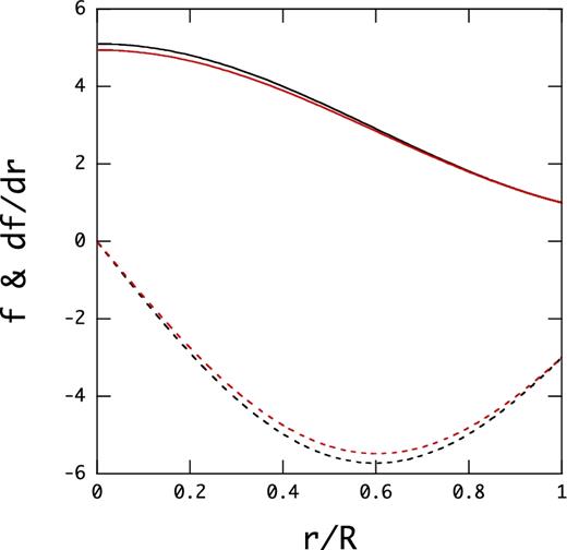
Functions f (solid lines) and df/dr (dotted lines) versus x = r/R for a polytrope of the index n = 1 for ζ0 = 0.01 (black lines) and ζ0 = 1 (red lines), where f and df/dr are normalized by BS ≡ μb/R3 and BS/R, respectively.
3.1 Spheroidal modes
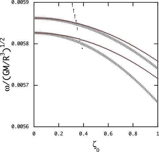
In Fig. 2 we plot |$\bar{\omega }$| of the first two spheroidal magnetic modes of even parity (left-hand panel) and of odd parity (right-hand panel) as a function of ζ0 for BS = 1014 G (red dots) and BS = 1015 G (short vertical lines), where we have used jmax = 14 and |$10\times \bar{\omega }$| is plotted for BS = 1014 G. The figure suggests that the frequency of the spheroidal magnetic modes is almost exactly proportional to the field strength BS for ζ0 ≲ 1. We find δcs ∼ 10−3 for even parity modes and δcs ∼ 10−2 for odd parity modes, that is, odd parity modes show rather poor consistency compared to even parity modes. The figure also shows that as the parameter ζ0 increases the frequency |$\bar{\omega }$| decreases and that the magnetic modes sometimes suffer avoided crossings with other magnetic modes. We find that the consistency δcs becomes poor at such avoided crossings.
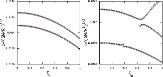
Eigenfrequency |$\bar{\omega }$| of the first two magnetic modes of even parity (left-hand panel) and odd parity (right-hand panel) versus ζ0 for BS = 1015 G (short vertical lines) and BS = 1014 G (red dots), where the frequency |$10\times \bar{\omega }$| is plotted for BS = 1014 G.
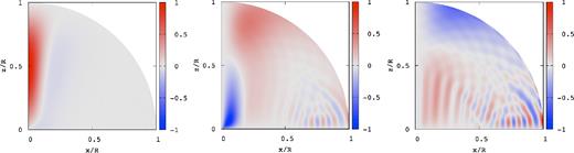
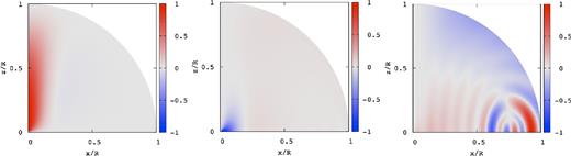
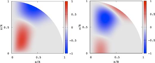
Wave patterns |$\hat{\xi }_r$| (left-hand panel), |$\hat{\xi }_\theta$| (middle panel), and |$\hat{\xi }_\phi$| (right-hand panel) for the spheroidal magnetic mode of even parity for BS = 1015 G at ζ0 = 0.01, where |$\bar{\omega }=1.426\times 10^{-2}$|.
Fig. 4 shows the patterns |$\hat{\xi }_j$| for the same mode as in Fig. 3 but for ζ0 = 1, where the frequency is |$\bar{\omega }=1.392\times 10^{-2}$|. The patterns of |$\hat{\xi }_r$| and |$\hat{\xi }_\theta$| at ζ0 = 1 are almost the same as those at ζ0 = 0.01. The pattern |$\hat{\xi }_\phi$| at ζ0 = 1, however, is significantly different from that at ζ = 0.01, and the short wavy patterns found for ζ0 = 0.01 disappear for ζ0 = 1. Note that the amplitude of ξϕ at ζ0 = 1 is comparable to those of ξr and ξθ.
Same as Fig. 3 but for ζ0 = 1, where |$\bar{\omega }=1.392\times 10^{-2}$|.
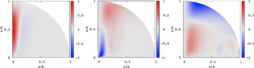
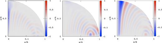
Figs 5 and 6 show the patterns of |$\hat{\xi }_j$| for the odd magnetic mode at ζ0 = 0.01 and ζ0 = 1, where the frequency is |$\bar{\omega }=5.846\times 10^{-3}$| for the former and |$\bar{\omega }=5.704\times 10^{-3}$| for the latter. The pattern |$\hat{\xi }_r$| is antisymmetric and those of |$\hat{\xi }_\theta$| and |$\hat{\xi }_\phi$| are symmetric about the equator for odd modes. Interestingly, no significant differences in the wave patterns |$\hat{\xi }_j$| are found between the cases of ζ0 = 0.01 and ζ0 = 1 although the amplitudes of ξϕ at ζ0 = 1 are by about a factor 100 larger than those at ζ0 = 0.01. The amplitudes of |$\hat{\xi }_r$| and |$\hat{\xi }_\theta$| are confined to the region along the magnetic axis, but |$\hat{\xi }_\phi$| has amplitudes in the whole interior except on the magnetic axis.
Wave patterns |$\hat{\xi }_r$| (left), |$\hat{\xi }_\theta$| (middle), and |$\hat{\xi }_\phi$| (right) for the spheroidal magnetic mode of odd parity at ζ0 = 0.01, where |$\bar{\omega }=5.846\times 10^{-3}$|.
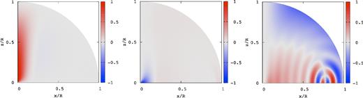
Same as Fig. 5 but for ζ0 = 1, where |$\bar{\omega }=5.704\times 10^{-3}$|.
3.2 Toroidal modes
In Fig. 7, |$\bar{\omega }$| of the toroidal magnetic modes is plotted as a function of ζ0, where the red dots and short vertical lines are for the cases of BS = 1014 G and 1015 G, respectively, and |$10\times \bar{\omega }$| is plotted for the former.1 The frequencies decrease with increasing ζ0, which behaviour is similar to that found for spheroidal magnetic modes, and we find δcs ∼ 10−3 for the toroidal modes except at and near the avoided crossings. The frequencies |$10\times \bar{\omega }$| for BS = 1014 G and |$\bar{\omega }$| for BS = 1015 G agree with each other only when ζ0 ≪ 1, and the agreement is lost as ζ0 increases, that is, except when ζ0 ∼ 0 the frequency of the toroidal magnetic modes does not linearly scale with BS, which is different from what we find for spheroidal magnetic modes. The toroidal magnetic modes are governed by the differential equations (22) and (23) and are described by the variables |${\boldsymbol y}_5$| and |${\boldsymbol y}_6$| when ζ0 = 0. As ζ0 increases from ζ0 = 0, however, the variables |${\boldsymbol y}_1$| and |${\boldsymbol y}_2$| come in and play a non-negligible role to determine the frequency in equations (22) and (23). Since the variables |${\boldsymbol y}_1$| and |${\boldsymbol y}_2$| are also affected by compressibility, which may be independent of the field strength B, the proportionality of the frequency of the toroidal modes with the field strength BS may be lost.
Eigenfrequency |$\bar{\omega }$| of the first two toroidal magnetic modes of odd parity versus ζ0 for BS = 1014 G (red dots) and BS = 1015 G (vertical short lines), where |$10\times \bar{\omega }$| is plotted for BS = 1014 G.
Figs 8 and 9 show the wave patterns |$\hat{\xi }_j$| for the toroidal modes at ζ0 = 0.01 and ζ0 = 1, respectively. We find no significant differences in the wave patterns between the two cases, and the amplitudes of ξϕ always dominate those of ξr and ξθ for ζ0 ≲ 1. These wave patterns may suggest that the eigenfunctions are not necessarily well converged for jmax = 14.
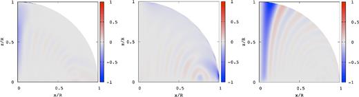
Wave patterns |$\hat{\xi }_r$| (left-hand panel), |$\hat{\xi }_\theta$| (middle panel), and |$\hat{\xi }_\phi$| (right-hand panel) for the toroidal magnetic mode of odd parity at ζ0 = 0.01 for BS = 1015 G, where |$\bar{\omega }=5.862\times 10^{-3}$|. The mode tends to the pure toroidal magnetic mode of odd parity as ζ0 → 0.
Same as Fig. 8 but for ζ0 = 1 where |$\bar{\omega }=5.741\times 10^{-3}$|.
4 CONCLUSION
We have computed axisymmetric magnetic modes of neutron stars magnetized by a mixed poloidal and toroidal field. For the mixed magnetic field (|$\zeta _0\not=0$|), axisymmetric spheroidal and toroidal modes are coupled. Calculating magnetic modes as a function of ζ0 from 0 to ∼1, we find that the frequency decreases with increasing ζ0 and that they suffer avoided crossings with other magnetic modes as ζ0 changes. We also find that the frequency of the spheroidal magnetic modes is almost exactly proportional to BS for ζ0 ≲ 1. The amplitude of ξϕ of the spheroidal magnetic modes is roughly proportional to ζ0 and become comparable to those of ξr and ξθ when ζ0 ∼ 1. For toroidal magnetic modes, on the other hand, the proportionality of the frequency to BS holds only when ζ0 ≪ 1 and is lost with increasing ζ0, and ξϕ is always dominating the other components for ζ0 ≲ 1. We find no unstable modes of ω2 < 0 for axisymmetric magnetic modes.
We recognize several inconsistencies in our treatment of the oscillations of magnetized stars employed in this paper. First, we have ignored the equilibrium deformation due to magnetic fields. The magnitudes of magnetic deformation may be of order of B2, which is much smaller than the gas pressure in most of the interior region of the star, except for the case of extremely strong magnetic fields as strong as B ∼ 1018 G. Secondly, the discontinuity in Bϕ at the surface induces a surface current and hence the tangential force at the surface when |$B_r\not=0$|, which effects are not taken account of in our modal analyses.
As discussed in Appendix C, the surface boundary conditions can be very important to determine the modal property of pure toroidal modes of a neutron star possessing a pure poloidal magnetic field. For the surface boundary condition |$B^{\prime }_\phi =0$|, we obtain only eigenmodes having real ω and eigenfunctions. For the surface boundary condition |${\mathrm{\partial} (\xi _\phi /r)/\mathrm{\partial} r}=0$|, however, we find an eigenmode having complex ω and eigenfunctions as well as real eigenmodes which have converging wave patterns with increasing jmax. For this boundary condition, the force operator |${\boldsymbol F}({\boldsymbol\xi} )$| is not self-adjoint and may permit complex modes. The boundary condition |${\mathrm{\partial} (\xi _\phi /r)/\mathrm{\partial} r}=0$| may be used to satisfy the condition that the traction vanishes at the surface of a solid crust. This may suggest that if we consider a neutron star with a solid crust the property of the toroidal magnetic modes in the fluid core could be significantly different from what we have found in this paper. Besides, if a neutron star has a solid crust, there exist spheroidal and toroidal sound waves travelling in the solid crust. It is interesting for us to examine how the sound waves in the solid crust will be affected by introducing the toroidal magnetic field since the toroidal sound waves are possibly coupled with Alfvén modes in the core and could be quickly damped (e.g. Levin 2006, 2007). Whether or not this strong damping of the crustal modes is still relevant for mixed poloidal and toroidal field configurations is a question to be answered in terms of normal mode analyses (e.g. Colaiuda & Kokkotas 2012 in terms of MHD simulations).
Introducing the toroidal magnetic field, the spheroidal component of the displacement vector of even parity is coupled with the toroidal component of odd parity and vice versa. In the case of rotating stars, however, the Coriolis force couples the even (odd) spheroidal component with even (odd) toroidal component of the displacement vector. This means that if we consider rotating stars magnetized by mixed poloidal and toroidal fields, the perturbations are not separated into two different mode groups according to the parity, which probably makes it difficult to analyse the modal properties of magnetized stars.
For mixed poloidal and toroidal magnetic field configurations, which are more favorable for magnetized stars from the stability point of view, toroidal (axial) and spheroidal (polar) components of the velocity fields of the perturbations are coupled even for axisymmetric modes of non-rotating stars. In this paper, we show that spheroidal and toroidal magnetic modes are separately obtained as discrete normal modes even with the coupling between them. Because of the coupling, toroidal magnetic modes are accompanied by density perturbations, which could affect the stability and hence the lifetime of the toroidal modes. We have to take account of the effects of a solid crust on the magnetic modes to closely compare our results to those by Colaiuda & Kokkotas (2012). It is also interesting to examine whether or not the coherent magnetic modes discussed by Gabler et al. (2016) and Passamonti & Pons (2016) can be regarded as normal modes. These will be among our future projects.
Footnotes
At ζ0 = 0, axisymmetric toroidal modes and spheroidal modes are decoupled. We have computed axisymmetric toroidal modes for ζ0 = 0 using the surface boundary conditions |${\boldsymbol y}_6=0$| and |${\rm d}{\boldsymbol y}_5/{\rm d}r=0$|, and the frequency |$\bar{\omega }$| of the magnetic toroidal modes for BS = 1015 G is tabulated for the two boundary conditions in Table C1 in Appendix C.
REFERENCES
APPENDIX A: EQUILIBRIUM MAGNETIC FIELDS
APPENDIX B: SURFACE BOUNDARY CONDITIONS
APPENDIX C: TOROIDAL MODES FOR POLOIDAL MAGNETIC FIELDS
Wave patterns |$\hat{\xi }_\phi$| (left) and |$\hat{B}^{\prime }_\phi$| (right) of the pure toroidal magnetic mode of odd parity for BS = 1015 G, where |$\bar{\omega }=1.923\times 10^{-2}$|.
Eigenfrequency |$\bar{\omega }$| of pure toroidal magnetic modes for BS = 1015 G for two different surface boundary conditions, where the largest eigenfrequency for a given number of radial nodes is tabulated.
| Parity | Number of radial nodes | ||
|---|---|---|---|
| 0 | 1 | 2 | |
| |$B^{\prime }_\phi =0$| | |||
| Odd | 5.862 × 10⁻³ | 1.918 × 10⁻² | 3.176 × 10⁻² |
| Even | ⋅⋅⋅ | ⋅⋅⋅ | ⋅⋅⋅ |
| |${\mathrm{\partial} (\xi _\phi /r)/\mathrm{\partial} r}=0$| | |||
| Odd | ⋅⋅⋅ a | 1.923 × 10⁻² | 3.186 × 10⁻² |
| Even | ⋅⋅⋅ | ⋅⋅⋅ | 2.556 × 10⁻² |
Note. aWe obtain |$\bar{\omega }=7.188\times 10^{-3}\pm 2.73\times 10^{-4}{\rm i}$| for jmax = 14.
