


Abstract
We report results from 21-cm intensity maps acquired from the Parkes radio telescope and cross-correlated with galaxy maps from the 2dF galaxy survey. The data span the redshift range 0.057 < z < 0.098 and cover approximately 1300 deg2 over two long fields. Cross-correlation is detected at a significance of 5.7 σ. The amplitude of the cross-power spectrum is low relative to the expected dark matter power spectrum, assuming a neutral hydrogen (H i) bias and mass density equal to measurements from the ALFALFA survey. The decrement is pronounced and statistically significant at small scales. At k ∼ 1.5 h Mpc−1, the cross-power spectrum is more than a factor of 6 lower than expected, with a significance of 15.3 σ. This decrement indicates a lack of clustering of neutral hydrogen (H i), a small correlation coefficient between optical galaxies and H i, or some combination of the two. Separating 2dF into red and blue galaxies, we find that red galaxies are much more weakly correlated with H i on k ∼ 1.5 h Mpc−1 scales, suggesting that H i is more associated with blue star-forming galaxies and tends to avoid red galaxies.
1 INTRODUCTION
Observations of neutral hydrogen (H i) provide a rich tool for understanding cosmology and astrophysics. Below z ∼ 6, the majority of hydrogen is reionized by stellar radiation except for dense clumps of H i that are self-shielded from ionizing and Lyman radiation. These clumps, the densest of which are known as Damped Lyman Alpha systems (DLAs), are highly correlated with matter over-densities, where gravitational collapse provides the requisite hydrogen density for self-shielding. They are also thought to be crucial to star formation, since stars are unlikely to gravitationally collapse from warm ionized gas and are instead expected to evolve from cold neutral clouds, to molecular clouds, to collapsed stars (Prochaska & Wolfe 2009). Measurements of neutral hydrogen therefore provide an opportunity to study star formation and to trace matter perturbations on large cosmic scales.
Several techniques exist to measure the H i density from redshifts of 0 to about 6. Above z ∼ 2.2, the Lyman alpha line is redshifted to optical frequencies, and H i regions can be detected in absorption features from distant quasars (Prochaska & Wolfe 2009). This technique has a maximum redshift of about 6, however, at which point the hydrogen neutral fraction seems to have been high enough for complete absorption of the quasar spectrum (Gunn–Peterson troughs). Below z ∼ 2.2, the Lyman alpha line moves into the ultra-violet, and atmospheric scattering makes ground-based measurements difficult. A more suitable method at low redshifts is to use the 21-cm emission line of H i.
At very low redshifts, individual galaxies can be detected via blind searches for spikes in 21-cm emission. The H i Parkes All Sky Survey (HIPASS) (Meyer et al. 2004) and Arecibo Legacy Fast ALFA (ALFALFA) (Haynes et al. 2011) survey used this technique to detect individual galaxies out to z ∼ 0.04 and z ∼ 0.06, respectively. However, blind galaxy searches become impractical at higher redshifts, since larger collecting areas are required to detect more distant galaxies. Higher redshift detections of individual galaxies, out to z ∼ 0.2, can still be made by pointing telescopes at known galaxy positions, but this requires long integration times to overcome thermal noise. The sky coverage of this method can be extended if one abandons the requirement of detecting individual galaxies. Instead, one can measure the 21-cm signal from the known locations and redshifts of many galaxies and boost the signal-to-noise ratio by co-adding them. This technique is known as galaxy stacking, and it can yield high signal-to-noise ratio measurements of the typical H i mass of optically selected galaxies. It is difficult to use galaxy stacking to determine the global H i content, especially at high redshift, since galaxy surveys will omit some of the optically dim H i galaxies. However, stacking was used to infer the comoving H i density at z < 0.13 (Delhaize et al. 2013) and at z = 0.24 (Lah et al. 2007).
A promising new technique is known as 21-cm intensity mapping. Instead of cataloguing individual galaxies, one can make low-resolution three-dimensional maps of the large-scale structure (LSS) directly by detecting fluctuations in the aggregate 21-cm emission. Such surveys can be quickly carried out by radio telescopes and can, in principle, constrain the equation of state of dark energy by measuring the baryon acoustic oscillation feature to high accuracy (Chang et al. 2008). Because individual galaxies do not need to be identified, intensity mapping does not require telescopes with extremely large collecting areas in order to extend to high redshifts. Another advantage of intensity mapping is that it is sensitive to emission from H i systems of all sizes. This feature contrasts with blind searches for H i galaxies, which are biased towards galaxies with large H i masses. Cross-correlating intensity mapping surveys with galaxy surveys works similarly to galaxy stacking, but the aim is to measure clustering by analysing the full correlation function or power spectrum of the 21-cm and galaxy maps.
The chief difficulty for 21-cm intensity mapping is the presence of radio point sources and free–free and synchrotron emission from the Galaxy. These foregrounds are two to three orders of magnitude brighter than the H i signal at z < 1. Fortunately, the inherent smoothness of the frequency spectrum of foregrounds (Liu & Tegmark 2012) contrasts with the clumpy 21-cm signal that traces the redshift distribution of matter perturbations. In the absence of instrumental effects, foregrounds could be removed by subtracting a slowly varying signal along the line of sight. However, telescopes convert the inherently smooth foregrounds to more complicated functions of frequency through imperfect bandpass calibration and frequency-dependent beam patterns, and these instrumental effects necessitate the use of more sophisticated techniques to remove the foreground signal. In 2009, Pen et al. (2009) reported the first detection of cosmic structure using 21-cm maps from the HIPASS survey cross-correlated with the 6dF galaxy redshift survey (Jones et al. 2004). The correlation function was measured over a small range of separations, from 0 to 3 Mpc. In the Northern hemisphere, the only 21-cm intensity mapping detection has come from H i maps from the Green Bank Telescope (GBT) cross-correlated with the WiggleZ and DEEP galaxy surveys at z ∼ 0.8, using either Principal Component Analysis (PCA) (Chang et al. 2010; Masui et al. 2013) or Independent Component Analysis (ICA) (Wolz et al. 2016b) to remove the foregrounds in the radio maps. These measurements probed a much greater range of scales than the Pen et al. (2009) correlation function.
Here, we present the cross-power spectrum of 21-cm intensity maps from the Parkes Observatory correlated with the 2dF galaxy survey at z ∼ 0.08. This result is the first 21-cm intensity mapping result in the Southern hemisphere to detect clustering at scales larger than 3 Mpc. It demonstrates the robustness of the PCA foreground removal technique, which is shown to work for a multi-beam instrument with a different bandpass and beam shape from the GBT. The redshift range of the Parkes measurement (0.057 < z < 0.098) is significantly lower than the GBT measurement (0.6 < z < 1), so a comparison of the two constrains the redshift evolution of the H i power spectrum. The Parkes maps also probe smaller scales than the GBT measurement, which provides an opportunity to probe the mid-scale clustering characteristics of H i.
2 OBSERVATIONS
The Parkes 21-cm Multi-beam Receiver (Staveley-Smith et al. 1996) was used to map the two large contiguous fields of the 2dF Galaxy Redshift Survey (Colless 1999) during a single week in late April and early May of 2014. During that week, 152 h (1976 beam hours) of data on the two 2dF fields were collected. The Multibeam Correlator (MBCORR) backend was used with a 64 MHz bandwidth centred at 1315.5 MHz, a 62.5 kHz frequency bin size, and 2 s integration times. Due to high variance at the edges of the band, the lowest 10 MHz and highest 4 MHz were removed from the final cross-power spectrum analysis described in Section 4. The results therefore cover a redshift range of 0.057 < z < 0.098. High variance and odd bandpass shapes were immediately evident in data from two of the YY beams and one of the XX beams (XX and YY refer to the two orthogonal linear polarizations); data from these polarizations and beams were therefore not used in any of the analysis. To minimize spurious signals from ground pickup, the telescope was positioned at a constant elevation angle during each field transit and scanned back and forth in azimuth as the field drifted through. Scans were made as the fields were rising and setting. The radio maps corresponding to the 2dF field near the North Galactic pole (NGP) cover roughly 4h30΄ in right ascension and 11° in declination, centred at 12h and 0°. The radio maps corresponding to the 2dF field near the South Galactic pole (SGP) cover roughly 6h30΄ in right ascension and 7° in declination, centred at 0h40΄ and −30°.
3 DATA ANALYSIS
In this section we describe all the steps to go from raw data to calibrated maps in which spectrally smooth astrophysical foregrounds have been mostly removed, such that the remaining fluctuations are at the thermal noise level. Section 3.1 describes RFI removal and map-making. Section 3.2 describes the bandpass and flux calibration procedure. Section 3.3 describes the procedure for removing the smooth astrophysical foregrounds.
3.1 Map-making
The raw data from MBCORR is stored in 3-min blocks. The first stage of our data analysis is a rough block-by-block cut to mitigate contamination by terrestrial sources of RFI. The high intrinsic spectral resolution of the data, 1024 channels across 64 MHz of bandwidth, allows for efficient identification and flagging of RFI. Individual frequency channels are flagged and removed if their variance, calculated across the duration of the block, is an extreme outlier compared to that of the other channels. Any RFI in a block that is not prominent enough to be flagged will contribute to a larger thermal noise estimation in the map-making stage, causing that block to be down-weighted when the map is made.
After RFI removal, the data are rebinned to 1 MHz bands (corresponding to a voxel depth of roughly 2.5 h−1 Mpc at band centre). For each 3-min block, the mean and slope in time are subtracted from the raw data, since these long time-scale modes are contaminated by 1/f noise. The timestream data are then converted to sky maps via an inverse-noise-weighted chi-squared minimization. This procedure has been used for CMB map-making (method 3 of Tegmark 1997), and it produces the maximum likelihood estimate of the sky map if the noise is Gaussian.
The noise covariance matrix is modelled in frequency-time space. The model assumes no frequency correlations, and it allows for correlations in time, but only within each block. Since there are no correlations between different blocks, the noise covariance matrix is estimated separately for each block. Two pieces go into this estimate. First, the thermal noise is estimated from the time variance of the data over the block and is placed on the diagonal. Secondly, the mean and slope subtraction is accounted for in the noise model by adding large noise to orthogonal mean and slope modes in the time portion of the noise covariance. This procedure allows the map-making algorithm to vary the mean and slope of each block to ensure maximum consistency between overlapping blocks. Since data were collected on multiple days and at both rising and setting times, all the maps are built from a web of multiple overlapping blocks (the overlapping rising and setting scans can be seen in the inverse-noise weights of Fig. 1). The multiple overlaps allow the map-making algorithm to distinguish real slowly varying structure on the sky from spurious variations that are caused by 1/f noise or by the mean and slope subtraction. The map-making algorithm also produces an inverse-noise covariance matrix in map space, based on the noise model just described. The diagonal is kept for use as noise weights for the subsequent calibration, foreground removal, and power spectrum calculations. For additional details on the map-making algorithm, see Masui (2013).

The two 21-cm sub-maps that overlap the 2dF SGP field are shown at band centre (the sub-maps that overlap the NGP field are not shown.). The three rows from top to bottom show: the maps before any foreground modes are removed; the maps after 10 modes are removed; and the inverse-noise weights, which are roughly proportional to the time spent observing each pixel. The colour scales, from left to right, refer to the maps from top to bottom. All beams have been combined, and the resolution has been degraded to 1.4 times the original beamsize. The point sources and diffuse galactic foregrounds have been strongly suppressed in the foreground-cleaned maps, and the scale of the remaining fluctuations is consistent with thermal noise. It should be noted that the fluctuations on the right ascension edges of the cleaned maps saturate the scale, but their magnitude is consistent with thermal noise and sparse coverage. Some cross-hatched striping can be seen in the maps and weights due to the differing scan angles of the azimuthal scan strategy as the field rose and set. The noise implied by the weights is higher than thermal noise because the mapmaker's noise estimation includes variance from the noise-cal measurement, residual RFI, and fluctuating foregrounds.
The map-making pipeline is based upon the pipeline used by Masui et al. (2013). However, the larger size of the Parkes fields necessitated the development of parallel processing tools to overcome memory and speed issues. Even with the parallelized code, it is necessary to break the two Parkes fields up into a total of four sub-maps. Map pixels are chosen to have a 0.08° width, which is approximately a third of the Parkes beam's full-width at half power (FWHP) of 0.25° at band centre. This FWHP corresponds to approximately 1 h−1 Mpc. Each submap location is mapped separately for each beam and polarization. This is necessary because bandpass calibration is performed after map-making, and each beam and polarization has a slightly different bandpass shape. After bandpass calibration and foreground cleaning, the separate beam maps are co-added with inverse-noise weights. Fig. 1 shows the calibrated maps of the SGP field before and after foreground removal, along with the inverse-noise weights, after all beams have been co-added.
3.2 Bandpass and flux calibration
A successful observation with a radiometer must (i) protect against fluctuations in the gain of the amplifiers, (ii) account for the bandpass spectrum (from frequency-dependent gain and bandpass filtering) that multiplies the true sky signal, and (iii) calibrate the total power by, for example, periodically observing astronomical sources of known brightness. In this section, we describe how we implement these steps.
The bandpass has three effects on the data. The most significant effect is a systematic multiplication of the true sky spectrum by the average bandpass shape. Secondly, fluctuations in the bandpass create noise in addition to the intrinsic thermal noise of the receiver. Finally, there is an effect where the presence of bright point sources adds ripples to the bandpass shape due to standing waves between the receivers and the dish [see section 3.5 of Calabretta, Staveley-Smith & Barnes (2014) for a discussion of this effect for Parkes]. Our bandpass calibration scheme aims only to estimate the average bandpass shape over the entire week long observation. Though it may be possible to account for variation of the bandpass over time by computing multiple bandpasses for different times, this risks biasing the data.
In preparation for the next stage of the analysis, we average maps from the two linear polarizations to form unpolarized maps. The 13 beams are then averaged, using their inverse-noise weights, into four groups. A: beams 1–3, B: beams 4–6, C: beams 7–9, and D: beams 10–13. Although group D appears to have data from more beams, two of the YY and one of the XX beams from that group are not included, because of high variance and strange bandpass shapes.
3.3 Foreground removal
Extragalactic point sources and the Milky Way produce synchrotron emission that is two to three orders of magnitude brighter than the 21-cm signal. In the absence of instrumental effects, these foregrounds are thought to be spectrally smooth and easily separable from the signal (Liu & Tegmark 2012), occupying just a few spectral degrees of freedom. In practice, bandpass instability, frequency-dependent beam response, and leakage of polarized foregrounds into unpolarized signal all conspire to impart a complicated frequency structure on to the originally smooth foregrounds. More importantly, these effects can mix the local angular structure of the map into frequency structure at each pixel. Therefore, we assume that the spectral structure of the foregrounds is not known a priori and must be determined from the data. Since the foregrounds are the dominant component in the maps, we determine these foreground modes via a PCA of the maps.
Although the frequency modes with the highest singular values are dominated by foregrounds, there will inevitably be loss of 21-cm signal when these modes are removed from the maps. This loss of power must be accounted for in the cross-power spectrum by the application of a transfer function, as described in Section 4.
4 POWER SPECTRUM ESTIMATION
In this section, we describe our method for estimating the cross-power spectrum between our foreground-cleaned 21-cm intensity maps and the 2dF galaxy overdensity maps. In order to compensate for signal loss from the foreground cleaning and to estimate error bars, we simulate the dark matter power spectrum and draw mock galaxy and H i maps from this simulation. We then use a Monte Carlo method to calculate the error bars, running 100 of these simulated galaxy and H i maps through our power spectrum pipeline. Section 4.1 describes these simulations, and Section 4.2 describes the estimation of the cross-power spectrum and its errors.
4.1 Simulations
For the next stage of the analysis, the simulated maps must be converted to telescope coordinates of frequency, right ascension, and declination. This requires a fiducial cosmology (we again use Planck 2015) and a gridding scheme. In order to preserve the z-axis as the line-of-sight direction, the conversion of transverse lengths into angular distances in right ascension and declination assumes a constant radial distance, independent of the redshift – for this purpose, the radial distance that halves the volume of the survey is chosen. The maps are then interpolated on to evenly spaced frequency intervals. An unclustered mock galaxy catalogue, following the survey selection function, is added to each galaxy over-density map to approximate the effect of galaxy shot noise. A set of galaxy density maps without this shot noise contribution is also kept. One set of the H i fluctuation maps is kept unaltered, and a second set is convolved with a Gaussian beam of width 1.4 times the largest Parkes beam, equal to the resolution of the common-beam-convolved real radio maps.
4.2 Cross-power spectrum
The procedure for estimating the cross-power spectrum of a pair of H i fluctuation and galaxy overdensity maps is as follows. First, the maps are multiplied by their weights: the selection function for the galaxy map, and the inverse-noise weights for the H i map. Then, they must be converted from right ascension, declination and frequency coordinates to physical comoving coordinates. This conversion is the reverse of the procedure described in the second paragraph of Section 4.1. The z-direction is chosen to be the line of sight. To convert angular distances to transverse distances, the same radius is used for all redshifts – the radius that halves the volume of the survey. This approximation results in a slightly distorted map that occupies a cube in Cartesian comoving coordinates, with the z-direction corresponding to the line-of-sight. Lastly, the map is interpolated on to evenly spaced coordinates in the z-direction.
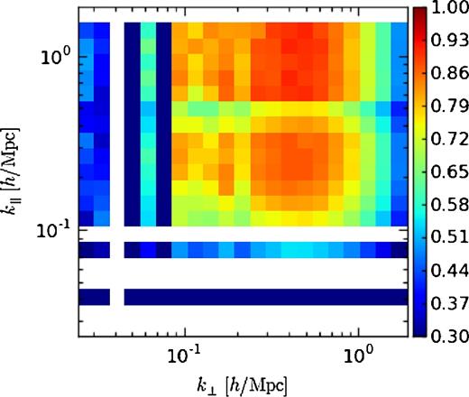
The Parkes-2dF transfer function, averaged over the four sub-maps, is shown above. The transfer function is a simulated estimate of the average fraction of H i-galaxy cross-power that is retained in 2D k-space after convolution with the Parkes beam and foreground subtraction. The foreground-cleaned Parkes-2dF cross-power spectrum is divided by the transfer function to compensate for signal loss. The lowest k∥ modes show strong signal loss, since the most prominent foreground modes found and removed by the SVD are smooth functions of frequency. On the right side of the figure, there is a smooth gradient of power loss towards high k⊥, due to the effects of beam convolution. The remaining structure, including the loss of power at low k⊥, is due to spurious correlations between the H i signal and the foregrounds. These spurious correlations perturb the SVD modes and cause additional power to be lost on spatial modes that overlap with the foregrounds and frequency modes that do not overlap with the foregrounds (Switzer et al. 2015).
To display our final results, we average the power spectrum to 1D bins. The average to 1D is weighted by the inverse variance of each k-bin across the 100 simulated recovered 2D power spectra. The observed cross-power spectrum, cleaned by removing 10 SVD modes, is shown in Fig. 3; we display only 1D Fourier modes for which we have full 2D angular coverage. The uncertainty assigned to each bin of the final observed 1D power is the corresponding standard deviation calculated from the 100 simulated 1D power spectra. The full covariance of the binned 1D power spectrum over the 100 simulations is also checked; we find no significant correlations, so the error bars at each point of Fig. 3 are independent. We list the standard deviations of the 2D power spectra in Appendix B. The inverse square of these are the weights used to bin to 1D power spectra. Each of the four sub-maps is analysed independently of the others – the final result is an average of these.

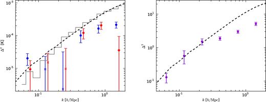
Left: observed 1D cross-power averaged over the four Parkes fields and cleaned by removing 10 SVD modes. A circle denotes positive power and a × denotes negative power. The grey line is the mean of the simulations, for which we assume |$b_{\rm H\,\,{\small I}} = 0.85$| and Tb = 0.064 mK, given by the ALFALFA measurement of |$\Omega _{\rm H\,\,{\small I}}$| (Martin et al. 2010). The dashed black line is the corresponding dark matter power spectrum scaled as equation (A1). Plotted error bars are 1σ, derived from the Monte Carlo simulations described in Section 4. Right: the purple points are the average of the auto-power spectra of the 2dF galaxies in the regions that overlap our Parkes maps. Errors are the standard deviation of the mean over the four sub-map regions. The dashed black line is the simulated dark matter power spectrum. The solid grey line is the expected shot noise signal, simulated from 100 unclustered mock catalogues that follow the survey selection function. The green points are the 2dF auto-power data minus the simulated shot noise.
As a null test for correlations between residual foregrounds and 2dF galaxies, we randomly shuffle the redshift slices of our 21-cm maps and compute the cross-power spectrum between these shuffled maps and the 2dF maps – we find the cross-power is consistent with zero on all scales of interest.
5 RESULTS AND DISCUSSION
Let us now consider the degree to which H i and galaxies will correlate for each of these terms. Since galaxies and H i should both be contained within haloes, and the distribution of haloes will trace the underlying dark matter density field, we expect r2h ≈ 1. On the other hand, it is likely that H i and optically selected galaxies have a tendency to occupy different haloes. Hess & Wilcots (2013) studied the group membership of over 740 overlapping optical galaxies from SDSS and H i galaxies from ALFALFA. They found that only 25 per cent of H i galaxies appear to be associated with an optically identified group, compared to half of optical galaxies. This tendency for H i to occupy different haloes suggests that both shot noise and one-halo clustering may not correlate between H i and optically selected galaxy populations: we expect r1h < 1 and rSN < 1. Therefore, r is thought to be close to unity on large scales and to fall off on smaller scales, as shot noise and one-halo clustering begin to dominate the power spectrum.
Now, let us analyse our measured cross-power spectrum. As previously indicated, the dashed black line in the left panel of Fig. 3 shows the power spectrum of equation (15) (which includes no shot noise term) with r = 1. RSDs, which modify the power spectrum according to equation (A1), are also included; this curve is a binning of this distorted 2D cross-power to 1D with isotropic weights. The grey line shows the signal we would realistically expect to measure if our model were accurate. It represents the average recovered cross-power spectrum from the 100 simulated galaxy and H i map pairs, including the effects of our window function, thermal noise, residual foregrounds, galaxy shot noise, compensation for signal loss, and anisotropic weighting (see Appendix B). The error bars on the data points show the standard deviation of these 100 simulations. The deviations of the data from the grey line in the left panel of Fig. 3 indicate disagreement with the simple model of equations (15) and (A1). In summary, the cross-power is well below the expectation of our model at all scales except for the largest scale (k ∼ 0.07h Mpc−1). The two negative points between 0.1h Mpc−1 and 0.3h Mpc−1 are slightly troubling, since there is no physical reason to expect an anti-correlation between H i and optical galaxies on large scales. However, the deviations from zero are not very significant, and those points are consistent with low positive clustering, or even the simulation line at ∼2σ. However, the decrement from the model is statistically significant at the two highest k points. At k ∼ 0.8h Mpc−1, the signal is approximately 39 per cent of the model, and the significance of the decrement is 5.0 σ. At k ∼ 1.5h Mpc−1, the signal is approximately 15 per cent of the model, and the significance of the decrement is 15.3 σ. These significances are calculated by subtracting the measured data points from the average of the 100 simulations and dividing by the standard deviation of the 100 simulations. We estimate the total statistical significance of the detected cross-power by calculating χ2, using the error bars from our 100 simulations. This rules out the null hypothesis of zero cross-correlation to an equivalent Gaussian significance of about 4.2 σ. Since most of our data are on small scales where the linear bias model may fail, we do not attempt to fit any curve to our data.
For comparison, the right panel of Fig. 3 shows the auto-power spectrum of the 2dF galaxies that overlap our Parkes fields. We estimate the shot noise contribution to this power spectrum by averaging the power spectrum of 100 unclustered mock catalogues that follow the survey selection function; the shot noise estimate is the grey curve. The purple points show our calculated 2dF auto-power spectrum, and the green points show this same power spectrum after subtracting the estimated shot noise contribution. The galaxy power spectrum after shot noise removal shows a similar decrement in clustering at high k to the H i–galaxy cross-power spectrum, but the effect is not as drastic at the two highest k-bins. Our 2dF power spectrum roughly agrees with the graphed or tabulated 2dF power spectra of Cole et al. (2005) and Tegmark, Hamilton & Xu (2002) at the points where they overlap, but the overlap is mostly at low k. The smallest scales analysed in those papers are k ∼ 0.185h Mpc−1 and k ∼ 0.6h Mpc−1, respectively. The analysis of Percival et al. (2001) displays the ratio of the 2dF power spectrum to model fits, extending to k ∼ 1h Mpc−1. Their plots show a decrease in 2dF power relative to the models at small scales, which is similar to the effect that we find. However, they ascribe this effect to aliasing from coarse binning. Due to the rather coarse frequency binning of our maps, it is conceivable that aliasing is also responsible for some of the low power we observe at small scales. In order to test this, we bin the galaxy maps first to the same frequency resolution as our H i maps and then with a factor of 8 finer frequency resolution and calculate the power spectrum for both cases. We find a nearly identical galaxy power spectrum, indicating that aliasing is not an issue.
It is likely that some of the low H i-galaxy clustering that we see on small scales is due to the correlation coefficient dipping below 1, since shot noise and one-halo clustering become more prominent in the power spectrum at high k. A reasonable way to test this is to split the galaxies by colour, under the hypothesis that the H i content of red galaxies is lower than that of blue galaxies. If this hypothesis is true, we would expect the H i–red galaxy correlation coefficient to drop more rapidly at small scales than the H i–blue galaxy correlation coefficient. Following the k-corrected colour splitting method used in Cole et al. (2005), we split the 2dF galaxies into red and blue populations and analyse the H i–galaxy cross-power spectra. In our fields, red galaxies account for approximately a third of the total 2dF population, and blue galaxies account for two thirds. The cross-power spectra with the blue and red galaxies are shown in the left panel of Fig. 4. The two cross-powers are quite similar, except that there is significantly more power at k ∼ 1.5h Mpc−1 in the H i cross-power with the blue galaxies compared to the H i cross-power with the red galaxies. The statistical significance of the difference is about 2.4 σ. This result favours the picture that the cross-power spectrum of H i and optical galaxies at k ∼ 1.5h Mpc−1 is dominated either by shot noise or by the one-halo term. Shot noise and one-halo clustering is seen more strongly when correlating H i with blue galaxies because blue galaxies contain a much larger fraction of the H i and are more likely to occupy the same haloes. A χ2 test of the cross-power between the H i signal and the blue 2dF galaxies rules out the null hypothesis of zero cross-correlation to an equivalent Gaussian significance of 5.7 σ.
Similar to Fig. 3, but the 2dF galaxies have been split into red and blue populations. The 100 simulations, used to calculate the error bars and the transfer function, have their galaxy counts adjusted to the appropriate number for the red and blue splits, to capture the effect of increased shot noise. Left: observed 1D cross-power spectrum between the H i maps and the red and blue 2dF galaxies, averaged over the four Parkes fields and cleaned by removing 10 SVD modes. The red cross-power points are slightly offset on the k-axis, for ease of reading. Right: observed 1D 2dF red–blue galaxy cross-power spectrum averaged over the regions that overlap our Parkes maps. Errors are the standard deviation of the mean over the four sub-map regions.
The results of our H i cross-power spectra with red and blue galaxies are qualitatively consistent with the findings of Papastergis et al. (2013). Their analysis of the projected cross-correlation function and auto-correlation function of red and blue SDSS galaxies and H i-selected ALFALFA galaxies reveals that the H i–blue cross-correlation coefficient is close to unity at all scales. On the other hand, the H i–red cross-correlation coefficient is unity at large separations, but it begins to drop at separations smaller than ∼5h−1 Mpc, indicating that the presence of a red galaxy decreases the probability of finding a nearby H i-galaxy, relative to statistically independent dark matter tracers. As noted by Papastergis et al. (2013), this result may reflect the fact that red galaxies tend to preferentially inhabit high-density haloes (Zehavi et al. 2011), which usually have lower fractions of H i gas, as seen in studies of individual groups and clusters (Haynes & Giovanelli 1986; Solanes et al. 2002; Hess & Wilcots 2013), hydrodynamic simulations (Villaescusa-Navarro et al. 2016), and empirical fits to the halo mass function (Padmanabhan & Kulkarni 2016). A lack of H i mass for many red galaxies is also found in simulations by Wolz et al. (2016a), using a semi-analytical galaxy formation model run on the Millennium simulation. A cross-power spectrum analysis of this simulation reveals a similar scale-dependence and colour-dependence to the correlation coefficient.
The analysis of Papastergis et al. (2013) suggests that optically selected blue galaxies and H i galaxies tend to occur in the same environments or perhaps are the same galaxies. To test this, we plot the cross-power spectrum of red and blue galaxies on the right panel of Fig. 4, suspecting that it may be similar to the cross-power spectrum of H i and red galaxies. In fact, we find that the cross-power spectrum of red and blue galaxies is more similar to the full galaxy auto-power spectrum with shot noise subtracted. This makes sense, since the blue and red galaxies are disjoint sets. The side-by-side comparison of red--blue galaxy cross-power spectrum and the H i–red cross-power spectrum in Fig. 4 suggests that the overlap of H i with red galaxies is even weaker than the overlap of red and blue galaxies.
Three points can be drawn from our results. First, the small-scale clustering amplitude is much lower than the HALOFIT prediction, as seen in both the galaxy–H i power spectrum and the shot-noise-subtracted galaxy auto-power spectrum. Secondly, the galaxy–H i cross-correlation coefficient is scale-dependent and colour-dependent, probably due to one-halo clustering and shot noise. H i appears to be much more strongly associated with blue galaxies than red galaxies. Thirdly, H i-galaxy clustering may also be somewhat suppressed at 0.1h Mpc−1 and 0.3h Mpc−1 scales, though the statistical significance of this is not high.
6 CONCLUSIONS
We measure the cross-power spectrum between foreground-cleaned 21-cm intensity maps and 2dF galaxy maps at z ∼ 0.08. The cross-power spectrum is lower than the expected signal, if one assumes the ALFALFA values for the H i density and H i bias. The decrement compared to the model has high statistical significance at k ∼ 1hMpc−1. Despite the smaller than expected signal, the null hypothesis of no correlated clustering between H i and galaxies can be ruled out to a significance of 5.7 σ, using the cross-power spectrum of the 21-cm maps and the blue 2dF galaxies. The detection demonstrates the effectiveness of the SVD method for 21-cm foreground removal. A splitting of the galaxies by colour reveals that an extreme observed decrement in power at k ∼ 1.5h Mpc−1 is likely due to a scale-dependent correlation coefficient between H i and red galaxies that falls off sharply as shot noise and the one-halo term begins to dominate the clustering power. This supports the picture that the H i content of blue galaxies is much greater than the H i content of red galaxies. Constraints from the 21-cm auto-power spectrum will be the subject of future work.
ACKNOWLEDGEMENTS
The authors would like to thank Ettore Carretti for his assistance in operating and understanding the Parkes telescope. Computations were performed on the GPC supercomputer at the SciNet HPC Consortium. CJA acknowledges support from the Wisconsin Space Grant Consortium. CJA and PTT acknowledge support from NSF award AST-1211781. XC acknowledges support from MoST 863 grant 2012AA121701, NSFC Key Project 11633004, CAS project QYZDJ-SSW-SLH017.
REFERENCES
APPENDIX A: REDSHIFT-SPACE CROSS-POWER SPECTRUM
APPENDIX B: 2D WEIGHTS
The following two tables are the standard deviations of the 2D k-bins across 100 simulations per field, propagated through an average of the cross-power over the four Parkes fields; the corresponding inverse variance is used as weights for the 2D to 1D average. The first column in each table gives k∥ and the first row in each table gives k⊥.
| |$_{k_\parallel \backslash ^k{_\perp }}$| | 3.03e-02 | 3.72e-02 | 5.63e-02 | 6.93e-02 | 8.53e-02 | 1.05e-01 | 1.29e-01 | 1.59e-01 | 1.95e-01 | 2.40e-01 | 2.96e-01 | 3.64e-01 | 4.47e-01 | 5.50e-01 |
| 1.55e+00 | 7.10e-04 | 7.11e-04 | 6.26e-04 | 1.88e-03 | 1.29e-03 | 2.14e-03 | 2.47e-02 | 2.05e-03 | 1.06e-02 | 2.23e-03 | 1.96e-03 | 1.05e-03 | 8.26e-04 | 6.70e-04 |
| 1.26e+00 | 4.81e-04 | 9.84e-04 | 4.52e-04 | 1.39e-03 | 2.64e-04 | 2.44e-03 | 1.07e-03 | 9.37e-04 | 8.60e-04 | 6.68e-04 | 7.47e-04 | 5.30e-04 | 3.89e-04 | 2.71e-04 |
| 1.02e+00 | 3.32e-04 | 1.09e-03 | 2.70e-04 | 1.08e-03 | 5.16e-04 | 1.07e-03 | 1.05e-03 | 1.07e-03 | 8.69e-04 | 6.53e-04 | 5.09e-04 | 3.34e-04 | 3.49e-04 | 2.56e-04 |
| 8.33e-01 | 2.23e-04 | 5.09e-04 | 1.30e-04 | 1.09e-03 | 1.95e-04 | 6.84e-04 | 6.70e-04 | 5.61e-04 | 4.93e-04 | 3.77e-04 | 3.75e-04 | 2.80e-04 | 2.83e-04 | 2.28e-04 |
| 6.77e-01 | 2.41e-04 | 5.13e-04 | 1.49e-04 | 4.07e-04 | 1.39e-04 | 5.31e-04 | 5.62e-04 | 8.55e-04 | 5.11e-04 | 4.49e-04 | 3.92e-04 | 2.79e-04 | 2.40e-04 | 2.20e-04 |
| 5.50e-01 | 3.24e-04 | 7.12e-04 | 3.46e-04 | 3.41e-03 | 3.90e-04 | 8.22e-04 | 1.09e-03 | 9.12e-04 | 7.50e-04 | 6.81e-04 | 4.70e-04 | 3.58e-04 | 3.91e-04 | 3.04e-04 |
| 4.47e-01 | 9.20e-05 | 2.96e-04 | 2.00e-04 | 1.29e-03 | 2.92e-04 | 9.25e-04 | 5.67e-04 | 8.21e-04 | 4.89e-04 | 3.76e-04 | 3.13e-04 | 2.44e-04 | 3.32e-04 | 2.61e-04 |
| 3.64e-01 | 1.03e-04 | 2.11e-04 | 5.95e-05 | 2.16e-04 | 8.84e-05 | 6.03e-04 | 2.68e-04 | 2.63e-04 | 3.38e-04 | 2.13e-04 | 1.83e-04 | 1.81e-04 | 1.76e-04 | 1.54e-04 |
| 2.96e-01 | 1.16e-04 | 1.73e-04 | 6.24e-05 | 1.44e-04 | 7.23e-05 | 2.66e-04 | 2.19e-04 | 2.32e-04 | 2.35e-04 | 1.84e-04 | 1.49e-04 | 1.66e-04 | 1.74e-04 | 1.69e-04 |
| 2.40e-01 | 8.08e-05 | 1.36e-04 | 7.29e-05 | 1.30e-04 | 5.64e-05 | 3.71e-04 | 1.72e-04 | 1.63e-04 | 2.06e-04 | 1.38e-04 | 1.16e-04 | 1.39e-04 | 1.63e-04 | 1.65e-04 |
| 1.95e-01 | 4.92e-05 | 9.91e-05 | 3.13e-05 | 1.77e-04 | 4.19e-05 | 8.97e-05 | 2.08e-04 | 2.67e-04 | 2.45e-04 | 1.45e-04 | 1.30e-04 | 1.50e-04 | 1.76e-04 | 1.85e-04 |
| 1.59e-01 | 3.82e-05 | 5.31e-05 | 2.42e-05 | 7.26e-05 | 2.94e-05 | 4.18e-04 | 1.30e-04 | 1.49e-04 | 1.56e-04 | 1.27e-04 | 1.47e-04 | 1.66e-04 | 1.93e-04 | 2.16e-04 |
| 1.29e-01 | 2.65e-05 | 2.91e-05 | 2.22e-05 | 3.98e-05 | 2.16e-05 | 8.50e-05 | 8.63e-05 | 9.34e-05 | 1.06e-04 | 1.40e-04 | 1.66e-04 | 1.56e-04 | 1.90e-04 | 2.67e-04 |
| 8.53e-02 | 1.67e-05 | 1.70e-05 | 1.12e-05 | 3.72e-05 | 1.13e-05 | 3.76e-05 | 1.29e-04 | 9.07e-05 | 2.23e-04 | 2.64e-04 | 2.31e-04 | 1.95e-04 | 2.54e-04 | 4.18e-04 |
| 4.58e-02 | 6.07e-06 | 1.05e-05 | 5.18e-06 | 1.26e-05 | 1.09e-05 | 3.70e-05 | 1.06e-03 | 1.23e-04 | 1.89e-04 | 5.63e-03 | 7.43e-04 | 4.78e-04 | 6.71e-04 | 8.29e-04 |
| |$_{k_\parallel } \backslash ^{k_\perp }$| | 6.77e-01 | 8.33e-01 | 1.02e+00 | 1.26e+00 | 1.55e+00 | 1.91e+00 | 2.35e+00 | 2.89e+00 | 3.55e+00 | 4.37e+00 | 5.37e+00 | 6.61e+00 | 8.13e+00 | 1.00e+01 |
| 1.55e+00 | 5.02e-04 | 5.49e-04 | 4.66e-04 | 6.13e-04 | 7.10e-04 | 7.49e-04 | 1.34e-03 | 1.86e-03 | 3.09e-03 | 4.67e-03 | 7.70e-03 | 8.91e-03 | 1.39e-02 | 1.16e-02 |
| 1.26e+00 | 2.54e-04 | 2.53e-04 | 2.57e-04 | 2.46e-04 | 3.66e-04 | 3.80e-04 | 5.29e-04 | 8.89e-04 | 1.79e-03 | 3.19e-03 | 6.07e-03 | 2.13e-02 | 1.74e-02 | 2.15e-02 |
| 1.02e+00 | 2.43e-04 | 2.29e-04 | 2.36e-04 | 2.48e-04 | 2.66e-04 | 4.06e-04 | 6.14e-04 | 9.35e-04 | 3.31e-03 | 6.10e-03 | 1.04e-02 | 1.09e-02 | 1.91e-02 | 6.59e-02 |
| 8.33e-01 | 1.87e-04 | 1.95e-04 | 1.94e-04 | 2.11e-04 | 2.91e-04 | 4.03e-04 | 7.91e-04 | 1.21e-03 | 2.23e-03 | 5.59e-03 | 2.37e-02 | 7.82e-03 | 1.73e-02 | 5.11e-02 |
| 6.77e-01 | 2.08e-04 | 2.11e-04 | 2.23e-04 | 2.34e-04 | 3.46e-04 | 4.78e-04 | 7.96e-04 | 1.17e-03 | 3.35e-03 | 5.67e-03 | 8.62e-03 | 5.23e-02 | 3.28e-02 | 3.66e-02 |
| 5.50e-01 | 2.93e-04 | 2.97e-04 | 2.80e-04 | 3.97e-04 | 5.24e-04 | 8.20e-04 | 1.46e-03 | 2.13e-03 | 4.36e-03 | 7.02e-03 | 1.76e-02 | 1.87e-02 | 1.58e-01 | 6.49e-02 |
| 4.47e-01 | 2.42e-04 | 2.92e-04 | 2.93e-04 | 3.50e-04 | 5.29e-04 | 7.68e-04 | 1.32e-03 | 2.05e-03 | 3.78e-03 | 1.03e-02 | 1.66e-02 | 3.62e-02 | 2.91e-02 | 2.53e-01 |
| 3.64e-01 | 1.68e-04 | 2.21e-04 | 2.60e-04 | 3.93e-04 | 5.61e-04 | 7.63e-04 | 1.25e-03 | 2.06e-03 | 3.70e-03 | 1.36e-02 | 1.74e-02 | 2.65e-02 | 3.25e-02 | 4.44e-02 |
| 2.96e-01 | 1.97e-04 | 2.20e-04 | 3.39e-04 | 4.81e-04 | 5.99e-04 | 8.34e-04 | 1.31e-03 | 2.31e-03 | 5.94e-03 | 1.11e-02 | 2.01e-02 | 6.60e-02 | 6.60e-02 | 7.40e-02 |
| 2.40e-01 | 1.78e-04 | 2.47e-04 | 3.24e-04 | 4.48e-04 | 5.98e-04 | 8.72e-04 | 1.33e-03 | 2.59e-03 | 5.83e-03 | 1.17e-02 | 2.71e-02 | 2.32e-01 | 6.35e-02 | 1.11e-01 |
| 1.95e-01 | 2.17e-04 | 3.13e-04 | 3.53e-04 | 4.96e-04 | 6.98e-04 | 1.06e-03 | 1.53e-03 | 3.02e-03 | 6.04e-03 | 1.09e-02 | 2.40e-02 | 7.58e-02 | 2.46e-01 | 3.59e-02 |
| 1.59e-01 | 2.46e-04 | 3.27e-04 | 4.08e-04 | 5.20e-04 | 8.08e-04 | 1.28e-03 | 1.75e-03 | 3.06e-03 | 7.07e-03 | 1.19e-02 | 2.34e-02 | 3.14e-02 | 7.79e-02 | 4.52e-01 |
| 1.29e-01 | 2.99e-04 | 3.47e-04 | 4.70e-04 | 5.42e-04 | 9.46e-04 | 1.39e-03 | 2.09e-03 | 3.38e-03 | 6.97e-03 | 1.39e-02 | 2.38e-02 | 6.39e-02 | 4.89e-02 | 1.05e-01 |
| 8.53e-02 | 4.42e-04 | 5.22e-04 | 6.48e-04 | 8.54e-04 | 1.34e-03 | 2.06e-03 | 3.30e-03 | 6.02e-03 | 1.07e-02 | 2.05e-02 | 3.44e-02 | 8.34e-02 | 1.04e-01 | 1.11e-01 |
| 4.58e-02 | 8.50e-04 | 1.06e-03 | 1.30e-03 | 1.62e-03 | 2.58e-03 | 3.68e-03 | 5.70e-03 | 1.34e-02 | 2.16e-02 | 3.99e-02 | 5.74e-02 | 1.38e-01 | 1.58e-01 | 4.07e-01 |
