Model-independent cosmological constraints from growth and expansion

Abstract

1 INTRODUCTION

The discovery of the acceleration of the expansion of the Universe (Riess et al. 1998; Perlmutter et al. 1999) led to the emergence of the Λ cold dark matter (ΛCDM) paradigm, further supported by the study of the cosmological microwave background (Bennett et al. 2003; Planck Collaboration XIII 2016) and the large-scale structures of the Universe (e.g. Eisenstein et al. 2005; Alam et al. 2017). In this paradigm, gravity is described by general relativity (GR), and the energy budget is dominated by the cosmological constant as dark energy (DE), responsible for the acceleration of the expansion, and a smooth, cold dark matter component. However, the nature of DE is one of the biggest mysteries of modern physics, and the simplest candidate, the cosmological constant, poses theoretical problems (e.g. Weinberg 1989; Peebles & Ratra 2003). Alternatively, GR may not be the correct theory to describe gravity, and the acceleration may reflect departure from GR.

From equations (4) and (5), it is clear that fσ₈ depends on (Ω_m, γ, σ₈) and the expansion history h(z). In GR, γ ≃ 0.55, while modified theories of gravity such as f(R) (de Felice & Tsujikawa 2010) or DGP (Dvali, Gabadadze & Porrati 2000) predict different (possibly scale-dependent) values of γ (Linder & Cahn 2007). Therefore, fσ₈ is a powerful probe of gravity. Moreover, joined measurements of h(z) and fσ₈ can help break degeneracies between modified gravity theories and DE (Linder 2005, 2017). Therefore, it has been used to test the ΛCDM model or alternative gravity theories (e.g. Nesseris & Perivolaropoulos 2008; Bean & Tangmatitham 2010; Basilakos 2012; Shafieloo, Kim & Linder 2013; Gómez-Valent, Solà & Basilakos 2015; Ruiz & Huterer 2015; Mueller et al. 2016; Nesseris, Pantazis & Perivolaropoulos 2017; Solà, Gómez-Valent & de Cruz Pérez 2017).

In this paper, we aim to constrain some key cosmological parameters, namely, Ω_m, σ₈, and γ, by fitting the growth data using model-independent expansion histories that do not assume any DE model.

Section 2 describes the data and method, our results are shown in Section 3. Section 4 explores the effects of restricting the DE density to be positive at all redshift, and our conclusions are drawn in Section 5.

2 METHOD

We used reconstructed expansion histories from the Joint Light-curve Analysis (JLA; Betoule et al. 2014) and combined them with growth measurements.

2.1 Model-independent reconstructions of the expansion history

We should note that the method of smoothing we used in this work is in fact insensitive to the initial conditions and choice of the smoothing scale (cf. Shafieloo et al. 2006; Shafieloo 2007): whatever the initial conditions, the method converges to the solution preferred by the data. However, they will approach this final solution via different paths. The central idea of using the iterative smoothing in this work is to come with a non-exhaustive sample of plausible expansion histories of the Universe directly reconstructed from the data, therefore, we start the procedure with several initial conditions and combine the results at the end.

2.2 Combining the likelihoods

For each reconstructed h_n(z), we can calculate fσ₈ for some (Ω_m, γ, σ₈) by computing the integral in equation (5). We can thus explore the parameter space, and compare to growth measurements to obtain a χ² for the growth data. We used a compilation of growth data points from 2dF Galaxy Redshift Survey (2dFGRS; Song & Percival 2009), WiggleZ (Blake et al. 2011), 6dF Galaxy Redshift Survey (6dFGRS; Beutler et al. 2012), the VIMOS Public Extragalactic Redshift Survey (VIPERS; de la Torre & Peacock 2013), the Sloan Digital Sky Survey (SDSS) Main Galaxy Sample (Howlett et al. 2015), 2MASS Tully–Fisher (2MTF) survey (Howlett et al. 2017), and Baryon Oscillation Spectroscopic Survey (BOSS) Data Release 12 (DR12; Gil-Marín et al. 2017). We did not include the Subaru FMOS Galaxy Redshift Survey (FastSound) data (Okumura et al. 2016) at z = 1.4, since our smooth reconstructions do not reach that redshift.

The total |$\chi ^2_n$| for reconstruction n is thus |$\chi ^2_n = \chi ^2_{\mathrm{SN},n} + \chi ^2_{f\sigma _8,n}$|⁠. We can then find the parameters that minimize the χ², and their associated confidence intervals.

3 RESULTS

Using the reconstructed expansion histories h(z), we calculate the χ² as defined in Section 2.2. First, we fixed (γ, σ₈) = (0.55, 0.80), and allow Ω_m to vary. Since the reconstructed h(z) were obtained assuming a flat universe, Ω_m is allowed to vary between 0 and 1. For reference, we calculate the χ² of the ΛCDM model, and find its minimum |$\chi ^2_{\rm min, \Lambda CDM}$|⁠. We are interested in |$\Delta \chi ^2 = \chi ^2-\chi ^2_{\rm min, \Lambda CDM}$|⁠, the difference with respect to the best-fitting ΛCDM case. Fig. 1 shows |$\mathcal {L} = \exp (-\Delta \chi ^2/2)$| as a function of Ω_m for each reconstruction (in blue). Therefore, combinations of h and Ω_m with a better χ² than the best-fitting ΛCDM model (Δχ² < 0), have a likelihood larger than one. For comparison, we also show in red |$\mathcal {L}_{\rm \Lambda CDM} = \exp (-\Delta \chi ^2/2)$| for the ΛCDM case. The model-independent reconstructions seem to favour slightly lower Ω_m with respect to the ΛCDM case. However, they are fully consistent with the ΛCDM case.

Figure 1.

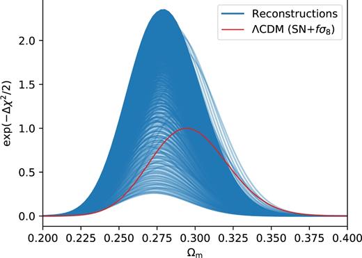
Exp(−Δχ²/2) (with respect to the best-fitting ΛCDM model) versus Ω_m for each reconstruction, fixing (γ, σ₈) = (0.55, 0.80). The red line shows the ΛCDM case.

Open in new tabDownload slide

We then allow γ or σ₈ to vary together with Ω_m, while fixing the third parameter to its fiducial value (σ₈ = 0.80 or γ = 0.55). In both cases, we calculate χ² for the ΛCDM case, and find the regions where Δχ² < 2.3 and Δχ² < 6.18, corresponding to 1σ and 2σ for 2 degrees of freedom. Fig. 2 shows in red the 1σ and 2σ regions of the ΛCDM case. For each model-independent reconstruction, we then calculate the χ² of the model-independent case, and find the regions in the (σ₈, Ω_m) and (γ, Ω_m) planes where the reconstructions give a better χ² than the best-fitting ΛCDM, namely, Δχ² < 0. Fig. 2 shows in blue the superposition of these regions over all reconstructions in the (Ω_m, σ₈) (left) and (Ω_m, γ) (right) planes. Therefore, if a point (σ₈, Ω_m) (or (γ, Ω_m)) is located in the blue region, there exists at least one reconstruction that, combined with (σ₈, Ω_m) (or (γ, Ω_m)), yields a better χ² than the best-fitting ΛCDM model.

Figure 2.

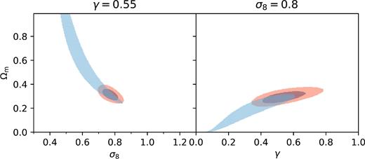
Superposition of the Δχ² < 0 (with respect to the best-fitting ΛCDM model) regions for γ = 0.55 (left) and σ₈ = 0.80 (right) in the model-independent case in blue. We also show in red the 1σ and 2σ regions of the ΛCDM model.

Open in new tabDownload slide

Fixing γ = 0.55 yields higher preferred values for Ω_m, while fixing σ₈ = 0.80 yields lower preferred values. However, the model-independent approach is fully consistent with ΛCDM. Moreover, it can be seen that, when h(z) is not restricted to ΛCDM, there is a stronger degeneracy in the parameters. Namely, it is possible to find expansions histories that, coupled with low values of Ω_m and γ, or with high values of Ω_m and σ₈, give a better fit to the combined data. The degeneracy in the parameters can be understood from equation (5): for fixed σ₈, |$\Omega _{\rm m}^\gamma$| should stay roughly constant, therefore lower Ω_m are compensated by lower γ. Similarly, for fixed γ, Ω_mσ₈ should stay constant, therefore lower Ω_m demand higher σ₈. This is consistent with the results of Shafieloo et al. (2013), with slightly tighter constraints.

Finally, we vary all three parameters (Ω_m, γ, σ₈) simultaneously. Fig. 3 shows in red the projections of the Δχ² < 3.53 and 8.02 regions of the ΛCDM case, corresponding to 1σ and 2σ for 3 degrees of freedom, on to the (σ₈, γ) (top-left), (σ₈, Ω_m) (bottom-left), and (γ, Ω_m) (bottom-right). For the model-independent case, we proceed as in Fig. 2, and find the Δχ² < 0 regions for each reconstruction. We then show in blue the projection on to the three planes of the superposition of the Δχ² < 0 regions over all reconstruction. Again, the blue region shows the region of the parameter space where there is at least one model-independent reconstruction that yields a better χ² than the best-fitting ΛCDM model.

Figure 3.

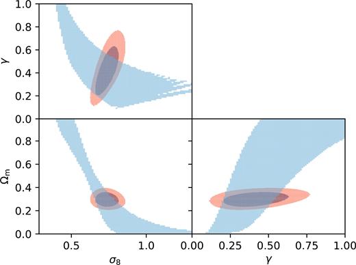
Superposition of the Δχ² < 0 (with respect to the best-fitting ΛCDM model) regions for (Ω_m, γ, σ₈) for the model-independent case (blue). In red we show the 1σ and 2σ regions for the ΛCDM case.

Open in new tabDownload slide

The model-independent joint constraints on (Ω_m, γ, σ₈) are now very broad. They are fully consistent with the ΛCDM model. The Δχ² < 0 region is consistent with both Ω_m = 0 and Ω_m = 1, while it allows γ between about 0.1 and 1, and σ₈ between 0.25 and 1.25.

4 DARK ENERGY CONSTRAINTS

Figure 4.

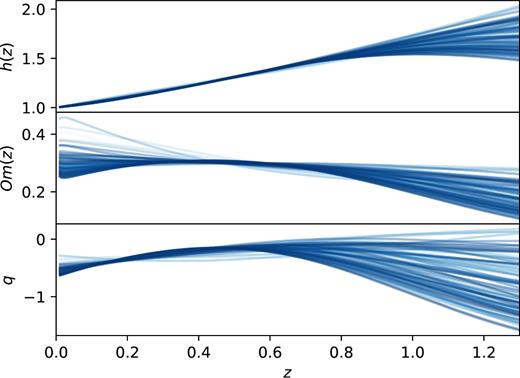
Reconstructed h(z), Om(z), and q(z). The colour code shows the index of the reconstruction.

Open in new tabDownload slide

The top and bottom panels of Fig. 5, respectively, show the matter density Ω_m(z) and the equation of state of DE for some combination of (Ω_m, h(z)) verifying the positivity condition (14), colour coded by the index of the reconstruction. The expansion histories that are closer from ΛCDM have a Om parameter close to constant, and their q(z) can cross 0, while some reconstructions further from ΛCDM do not cross 0. When Ω_m(z) crosses 1, equation (14) ceases to be valid, therefore none of the lines shown here cross 1.

Figure 5.

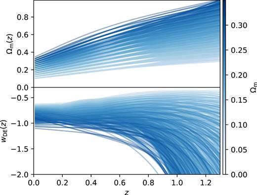
Reconstructed Ω_m(z) (top) and w(z) (bottom) for different Ω_m and h(z). All lines here verify equation (14).

Open in new tabDownload slide

We can now add the positivity condition (14) as a hard prior on Ω_m in the previous analysis. Indeed, large values of Ω_m combined with some reconstructions can lead to negative DE density, and these combinations should thus be rejected. Figs 6 and 7 show in blue the superposition over all reconstructions verifying equation (14) of the projected Δχ² < 0 regions of the parameter space. The red contours are unchanged with respect to Figs 2 and 3.

Figure 6.

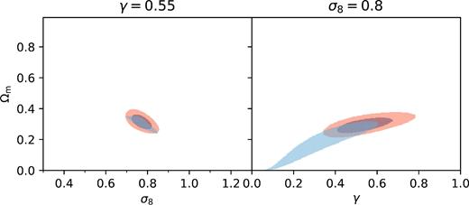
Blue: truncation of the Δχ² < 0 (with respect to the best-fitting ΛCDM model) regions for γ = 0.55 (left) and σ₈ = 0.80 (right) in the model-independent case using equation (14) as a hard prior. Red: 1σ and 2σ regions of the ΛCDM model.

Open in new tabDownload slide

Figure 7.

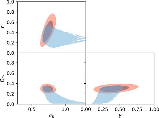
Blue: truncation of the Δχ² < 0 (with respect to the best-fitting ΛCDM model) regions for (Ω_m, γ, σ₈) for the model-independent case using equation (14) as a hard prior. Red: 1σ and 2σ regions of the ΛCDM case.

Open in new tabDownload slide

In Fig. 6, while the σ₈ = 0.8 case (right-hand panel) is not affected much, since it preferred lower values of Ω_m, the allowed region for the γ = 0.55 case is drastically reduced, and only a small space of the original Δχ² < 0 regions (i.e. before applying equation 14) is allowed. This region is located in the 2σ region of the ΛCDM case.

In Fig. 7, the Δχ² < 0 regions in each projection are also truncated with respect to Fig. 3, restricting the lower range of σ₈ and the higher range of γ and Ω_m.

The positivity condition (14) is thus a very strong constraint on the cosmological parameters, since it forbids large values of Ω_m ≳ 0.4. Indeed, for these values, the DE density crosses zero within our data range, therefore these values are not allowed here. On the other hand, for low enough values, Ω_DE(z) never crosses zero.

5 DISCUSSION AND CONCLUSION

Using model-independent reconstructions of the expansion history from Type Ia supernovae data, we fit the growth data and obtain constraints on (Ω_m, γ, σ₈). These model-independent constraints on the cosmological parameters are broader than the ΛCDM ones, but fully consistent. When all three cosmological parameter are let free, they are not well constrained, and it is possible to find expansion histories with cosmological parameters that are far from the ΛCDM constraints that give a reasonable fit to the data.

However, when restricting the combinations of Ω_m and the reconstructed expansion histories h(z) that yield a positive DE density parameter (h²(z) − Ω_m(1 + z)³ > 0), the constraints on the cosmological parameters become stronger. Moreover, when imposing GR, i.e. fixing γ = 0.55, the model-independent contours are truncated and fully contained within the ΛCDM ones, showing strong evidence in favour of ΛCDM. That is, combinations of large Ω_m with expansion histories that are too different from ΛCDM are excluded. It should be noted that in Linder (2005), γ depends on w following γ(w) = 0.55 + 0.05w(z = 1), therefore fixing γ = 0.55 is not completely model independent. However, we expect it to have little influence on the results presented here.

Our constraints are more stringent than Shafieloo et al. (2013) thanks to the better quality of the data and the introduction of the DE density positivity condition. The results are consistent with a flat ΛCDM Universe and gravity described by GR, although modified theories of gravity predicting different growth index cannot be ruled out at this stage. The combined χ² being currently dominated by the supernovae data, better growth measurements are needed to further constrain gravity theory.

Future surveys such as the Dark Energy Spectroscopic Instrument (DESI; DESI Collaboration et al. 2016) will bring down the errors on the growth measurements, while surveys such as the Wide Field Infrared Survey Telescope (WFIRST; Spergel et al. 2015) and the Large Synoptic Survey Telescope (LSST; Ivezic et al. 2008) are expected to observe thousands of supernovae, increasing the quality of the data and covering a larger redshift range.

ACKNOWLEDGEMENTS

We thank Eric Linder for useful discussions, and Teppei Okumura for providing us with the fσ₈ data. The computations were performed by using the high performance computing cluster Polaris at the Korea Astronomy and Space Science Institute. AS would like to acknowledge the support of the National Research Foundation of Korea (NRF-2016R1C1B2016478). The authors thank the Yukawa Institute for Theoretical Physics at Kyoto University. Discussions during the CosKASI-ICG-NAOC-YITP joint workshop YITP-T-17-03 were useful to complete this work.

REFERENCES

APPENDIX A: DATA VISUALIZATION

For visualization purpose, Fig. A1 shows some reconstructed fσ₈ verifying equation (14) and with |$\chi ^2<\chi ^2_{\rm \Lambda CDM}$|⁠.

Figure A1.

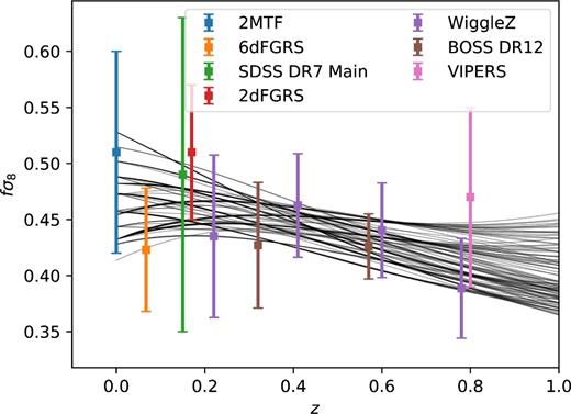
fσ₈ data and reconstructed fσ₈ with free (Ω_m, γ, σ₈). All lines shown here have |$\chi ^2<\chi ^2_{\rm \Lambda CDM}$|⁠.

Open in new tabDownload slide