


Abstract
Recent studies have presented evidence for tension between the constraints on Ωm and σ8 from the cosmic microwave background (CMB) and measurements of large-scale structure (LSS). This tension can potentially be resolved by appealing to extensions of the standard model of cosmology and/or untreated systematic errors in the modelling of LSS, of which baryonic physics has been frequently suggested. We revisit this tension using, for the first time, carefully calibrated cosmological hydrodynamical simulations, which thus capture the backreaction of the baryons on the total matter distribution. We have extended the BAryons and HAloes of MAssive Sysmtes simulations to include a treatment of massive neutrinos, which currently represents the best-motivated extension to the standard model. We make synthetic thermal Sunyaev–Zel'dovich effect, weak galaxy lensing, and CMB lensing maps and compare to observed auto- and cross-power spectra from a wide range of recent observational surveys. We conclude that: (i) in general, there is tension between the primary CMB and LSS when adopting the standard model with minimal neutrino mass; (ii) after calibrating feedback processes to match the gas fractions of clusters, the remaining uncertainties in the baryonic physics modelling are insufficient to reconcile this tension; and (iii) if one accounts for internal tensions in the Planck CMB data set (by allowing the lensing amplitude, ALens, to vary), invoking a non-minimal neutrino mass, typically of 0.2–0.4 eV, can resolve the tension. This solution is fully consistent with separate constraints from the primary CMB and baryon acoustic oscillations.
1 INTRODUCTION
It has long been recognized that measurements of the growth of large-scale structure (LSS) can provide powerful tests of our cosmological framework (e.g. Peebles 1980; Bond, Efstathiou & Silk 1980; Blumenthal et al. 1984; Davis et al. 1985; Kaiser 1987; Peacock & Dodds 1994). Importantly, growth of structure tests are independent of, and complementary to, constraints that may be obtained from analysis of the temperature and polarization fluctuations in the cosmic microwave background (CMB) and to so-called geometric probes, such as Type Ia supernovae (SNeIa) and baryon acoustic oscillations (BAOs, Albrecht et al. 2006).
The consistency between these various probes has been heralded as one of the strongest arguments in favour of the current standard model of cosmology, the Λcold dark matter (ΛCDM) model. The successes of the model, which contains only six adjustable degrees of freedom, are numerous and impressive. However, the quality and quantity of observational data used to constrain the model has been undergoing a revolution and a few interesting ‘tensions’ (typically at the few sigma level) have cropped up recently that may suggest that a modification of the standard model is in order.
One of the tensions surrounds the measured value of Hubble's constant, H0. Local estimates prefer a relatively high value of 73 ± 2 km s−1 Mpc−1 (Riess et al. 2016), whereas analysis of the CMB and BAOs prefer a relatively low value of 67 ± 1 km s−1 Mpc−1 (Planck Collaboration XIII 2016). A separate tension arises when one compares various LSS joint constraints1 on the matter density, Ωm, and the linearly evolved amplitude of the matter power spectrum, σ8, with constraints on these quantities from Planck measurements of the primary CMB. In particular, a number of LSS data sets (e.g. Heymans et al. 2013; Planck Collaboration XXIV 2016; Hildebrandt et al. 2017) appear to favour relatively low values of Ωm and/or σ8 compared to that preferred by the CMB data. (We summarize these constraints in detail in Section 2.) Our focus here is on this latter tension.
There are three (non-mutually exclusive) possible solutions to the aforementioned CMB–LSS tension: (i) there are important and unaccounted for systematic errors in the measurements of the primary CMB data; and/or (ii) there are remaining systematics in either the LSS measurements or in the physical modelling of the LSS data (e.g. inaccurate treatment of non-linear or baryon effects); and/or (iii) the standard model is incorrect. While exploration of measurement systematics in both the CMB and LSS data is clearly a high priority, significant focus is also being devoted to the question of LSS modelling systematics, as well as to making predictions for possible extensions to the standard model of cosmology. In this study, we zero in on these modelling issues.
We first point out that the different LSS tests (e.g. Sunyaev–Zel'dovich power spectrum, cosmic shear, CMB lensing, cluster counts, galaxy clustering, etc.) are just different ways of characterizing the ‘lumpiness’ of the matter distribution and how these lumps cluster in space. On very large scales (i.e. in the linear regime), perturbation theory is sufficiently accurate to calculate the matter distribution. However, most of the tests mentioned above probe well into the non-linear regime. The standard approach to modelling the matter distribution is therefore either to calibrate the so-called halo model using large dark matter cosmological simulations, or to use such simulations to empirically correct calculations based on linear theory (as in, e.g. the halofit package; Smith et al. 2003; Takahashi et al. 2012).
If the matter in the Universe was composed entirely of dark matter, such approaches would likely be highly accurate (assuming the analytic models could be accurately calibrated). However, baryons contribute a significant fraction of the matter density of the Universe and recent simulation work has shown that feedback processes associated with galaxy and black hole formation can have a significant effect on the spatial distribution of baryons, which then induces a non-negligible backreaction on the dark matter (e.g. van Daalen et al. 2011, 2014; Velliscig et al. 2014; Schneider & Teyssier 2015; Mummery et al. 2017; Springel et al. 2017). Until quite recently, such effects have typically been ignored when modelling LSS data, which might be expected to lead to significant biases in the inferred cosmological parameters (Semboloni et al. 2011). Recent cosmic shear studies (e.g. Hildebrandt et al. 2017), however, have attempted to account for the effects of baryons in the context of the halo model.
A separate modelling issue, which has so far attracted significantly less attention, is that the different LSS tests typically use quite different modelling approaches. For example, modelling of the galaxy cluster counts typically involves using parametrizations of the halo mass function from dark matter-only simulations, while modelling of galaxy clustering normally involves using the so-called halo occupation distribution (HOD) approach that takes relatively weak guidance from simulations, and modelling of weak lensing often uses linear theory with non-linear corrections. These differences likely reflect the fact that different aspects of the matter distribution are being probed by the different tests, but it does raise the important question of how appropriate it is to compare/combine the results of different LSS tests when they do not assume the same underlying matter distribution for a given cosmology.
Cosmological hydrodynamical simulations are the only method capable of self-consistently addressing the modelling limitations discussed above. Such simulations start from cosmological initial conditions and follow the evolution of matter into the non-linear regime, solving simultaneously for the gas, stellar, black hole, and dark matter evolution in the presence of an evolving cosmological background. The backreaction of the baryons on to the dark matter is therefore modelled self-consistently. As all of the important matter components are followed, it is possible to create virtual observations to make like-with-like comparisons with the full range of LSS tests, whether they are based on galaxies, the hot gas, or lensing produced by the total matter distribution. Hydro simulations therefore offer a means to address the issue of the lack of consistency in the modelling in different LSS fields.
As the simulations track star formation and black hole accretion, they also offer a means to account for the effects of ‘cosmic feedback’. This is a difficult problem though, as the feedback originates on scales that are too small to resolve with the kind of large-volume simulations required to do LSS cosmology. Therefore, one must employ physically motivated ‘subgrid’ prescriptions to take these processes into account. Recent studies have highlighted that many aspects of the simulations are more sensitive to the details of the subgrid modelling than one might hope (e.g. Schaye et al. 2010; Le Brun et al. 2014; Sembolini et al. 2016), calling into question their ab initio predictive power. On the positive side, however, one can learn about these processes by assessing which models give rise to systems that resemble those in the real Universe. Remarkable progress has been made in this regard recently, to the point where it is now possible to produce simulations that are difficult to distinguish from the real Universe in many respects.
Note that although current large-volume simulations lack the resolution to directly simulate the initiation of outflows on small scales (typically below scales of 1 kpc), the effects of feedback on larger scales can be directly simulated. This is relevant for LSS cosmology, where the typical length scales are >1 Mpc. Thus, if we can calibrate physically motivated prescriptions for the small-scale physics against observational constraints on some judiciously chosen properties, we can strongly increase the predictive power of the simulations for other observables. In other words, with calibration of physical feedback models we can strongly reduce the main theoretical limitation in current LSS cosmology tests.
This calibration approach is now being adopted by several groups in the theoretical galaxy formation field and has yielded significant progress (e.g. Vogelsberger et al. 2014; Schaye et al. 2015; Crain et al. 2015; Pillepich et al. 2018). The emphasis of these projects has been on simulating, at relatively high resolution, the main galaxy population (stellar masses of ∼108 − 11 M⊙). The simulations were calibrated on important galaxy properties (stellar masses and sizes in the case of EAGLE; Schaye et al. 2015) and it has been shown that they are able to reproduce other properties of the galaxy population quite well.
For LSS cosmology, much larger (and many more) simulations are required than considered previously. Additionally, while having realistic galaxy properties is clearly desirable, it is not sufficient to judge whether the feedback effects on LSS have been correctly captured in the simulations. That is because most of the baryons are not in the form of stars/galaxies, but in a diffuse, hot state. Thus, the simulations should reproduce the hot gas properties well if we are to trust the predictions for LSS.
In McCarthy et al. (2017, hereafter M17), we introduced the BAryons and HAloes of MAssive Sysmtes (BAHAMAS) simulations, which were designed specifically with LSS cosmology in mind. The stellar and active galactic nucleus (AGN) feedback prescriptions were carefully calibrated to reproduce the observed baryon fractions of massive systems (see Section 3), but M17 demonstrated that the simulations also reproduced an extremely wide range of observations, including the various observed mappings between galaxies, hot gas, total mass, and black holes. For example, the simulations reproduce the observed X-ray and thermal Sunyaev–Zel'dovich (tSZ) effect scaling relations of galaxy groups and clusters (including their intrinsic scatter), the thermodynamical radial profiles of the intracluster medium (density, pressure, etc.), the stellar mass–halo mass relations of galaxies and its split into centrals and satellites, the radial distribution of satellite stellar mass in groups and clusters, and the evolution of the quasar luminosity function.
Here, we employ the BAHAMAS simulations to revisit the claimed tension between LSS and the primary CMB. We focus here on comparisons to the tSZ effect, cosmic shear, CMB lensing, and their various cross-correlations. We also extend BAHAMAS to include a contribution from massive neutrinos to the dark matter, which has previously been proposed in a number of studies (e.g. Battye & Moss 2014; Beutler et al. 2014; Wyman et al. 2014) as a solution to the aforementioned tension. We constrain the summed mass of neutrinos, Mν, through the various LSS tests. In terms of the neutrino simulations, our approach to choosing the other relevant cosmological parameters (e.g. H0, Ωm, etc.) is to take guidance from primary CMB constraints and to assess which range of Mν, if any, can resolve the CMB–LSS tension (see Section 3.3).
This paper is organized as follows. In Section 2, we summarize the CMB–LSS tension and motivate our cosmological parameter selection strategy. In Section 3, we summarize the technical details of the BAHAMAS simulations and its calibration strategy. In Section 4, we explore the possible degeneracy between our feedback calibration strategy and cosmological parameter determination. In Section 5, we present our main results, based on comparing synthetic observations of the simulations to a wide variety of LSS observables. Finally, in Section 6, we summarize and discuss our findings.
2 CMB–LSS TENSION AND PREVIOUS CONSTRAINTS ON NEUTRINO MASS
A number of recent studies, which used simple analytic modelling2 of LSS, have found that there is presently tension between the constraints in the σ8 − Ωm plane derived from various LSS tests and that derived from the CMB, particularly so for the recent Planck results. (Note that σ8 is defined as the linearly evolved present-day amplitude of the matter power spectrum on a scale of 8 h−1 Mpc; i.e. it is the root mean square of the mass density in a sphere of radius 8 h−1 Mpc in linear theory.)
We summarize recent LSS constraints in Fig. 1. The four panels correspond to different LSS observables, including cosmic shear, tSZ effect statistics, galaxy clustering plus galaxy–galaxy lensing, and CMB lensing. In the top left panel, we show recent cosmic shear results from the CFHTLenS (Kilbinger et al. 2013; see also Heymans et al. 2013), Dark Energy Survey (DES) (Troxel et al. 2017), and Kilo Degree Surveys (KiDS, Hildebrandt et al. 2017) surveys. In the top right panel, we show various tSZ effect tests, including cluster number counts (Planck Collaboration XXIV 2016; de Haan et al. 2016), the power spectrum, one-point probability distribution function (PDF), and a combined analysis of the skewness and bispectrum of the Planck Compton y map (Planck Collaboration XXII 2016). Also shown are independent one-point PDF constraints from Atacama Cosmology Telescope (ACT) data (Hill et al. 2014). In the bottom left panel, we show recent combined galaxy clustering plus galaxy–galaxy lensing constraints using the SDSS main galaxy catalogue (Mandelbaum et al. 2013), SDSS main galaxy catalogue plus luminous red galaxies (Cacciato et al. 2013), SDSS BOSS galaxy clustering plus CFHTLenS lensing (More et al. 2015), and SDSS BOSS galaxy clustering plus CFHTLenS and CS82 weak-lensing data (Leauthaud et al. 2017). In the bottom right panel, we show constraints from modelling the Planck CMB lensing autocorrelation function (Planck Collaboration XV 2016) and the cross-correlation function between Planck CMB lensing and Planck tSZ effect maps (Hill & Spergel 2014). The curves represent the best-fitting power laws (derived by the original authors) describing the degeneracy between σ8 and Ωm for the data sets. There are two curves for each data set, representing the ±1σ uncertainties in the best-fitting amplitude of the power law. Note that for some of the tSZ effect tests (data points with errors), Ωm was held fixed at the (Planck) primary CMB best-fitting value and only σ8 was constrained by the data. Note also that, with the exception of the DES Y1 analysis, all of the LSS results presented in Fig. 1 were derived assuming either massless neutrinos or adopt the minimum mass (≈0.06 eV) allowed by oscillation experiments. The DES Y1 analysis allowed the summed neutrino mass to be a free parameter.
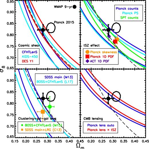
Summary of recent LSS constraints in the σ8–Ωm plane, compared with Planck 2015 primary CMB constraints (TT+lowTEB, closed contour repeated in each panel) and WMAP 9-yr primary CMB constraints (filled black circle with thick error bars). Top left: cosmic shear results from CFHTLenS, DES, and KiDS. Top right: various tSZ effect tests, including Planck 2015 cluster number counts, angular power spectrum, one-point PDF, and a combined analysis of the skewness and bispectrum of Planck 2015 Compton y map, a one-point PDF constraints from the ACT, and tSZ cluster count constraints from the SPT. Bottom left: combined galaxy clustering plus galaxy–galaxy lensing constraints from SDSS main galaxy catalogue (M13), SDSS main galaxy catalogue plus luminous red galaxies (C13), SDSS BOSS galaxy clustering plus CFHTLenS lensing (M15), and SDSS BOSS galaxy clustering plus CFHTLenS and CS82 weak-lensing data (L17). Bottom right: constraints from the Planck CMB lensing autocorrelation function and from the cross-correlation function between Planck CMB lensing and Planck Sunyaev–Zel'dovich effect maps. The curves represent the best-fitting power laws (derived by the original authors) describing the degeneracy between σ8 and Ωm for the different data sets. There are two curves for each data set, representing the ±1σ uncertainties in the best-fitting amplitude of the power law. To help compare the different LSS tests, we show in each panel, as the black dashed curve, a power law of the form S8 ≡ σ8(Ωm/0.3)1/2 = 0.77. The various LSS constraints consistently (at the ≈1σ–3σ level) point to lower values of σ8 at fixed Ωm (or lower values of Ωm at fixed σ8) compared to that derived from the most recent primary CMB data from Planck.
The various LSS constraints consistently, at the ≈1σ–3σ level, prefer lower values of σ8 at fixed Ωm (or lower values of Ωm at fixed σ8) compared to that derived from the most recent primary CMB data from Planck. The consistency amongst the different LSS tests is rather remarkable, given the very different nature of the tests involved, which probe different aspects of the matter distribution (i.e. galaxies versus hot gas versus total matter) at different redshifts and on different scales, each with their own differing sets of systematic errors. And note that the constraints shown in Fig. 1 do not form an exhaustive list. For example, other recent LSS tests, such as those based on the cross-correlations between CMB lensing and galaxy overdensity (Giannantonio et al. 2016), CMB lensing and cosmic shear (Liu & Hill 2015; Harnois-Déraps et al. 2017), and cosmic shear and the tSZ effect (Hojjati et al. 2015, 2017), also find qualitative evidence for tension (and in the same sense), but we do not plot them in Fig. 1, since they have not formerly quantified their best-fitting cosmological parameter values and their uncertainties.
The role that remaining systematics in either the analysis of the CMB (e.g. Spergel, Flauger & Hložek 2015; Addison et al. 2016; Planck Collaboration LI 2017) or that of LSS (such as the neglect of important baryon physics, which we will consider here) plays in this tension has yet to be fully understood. In spite of this, various extensions of the standard model have already been proposed to try to reconcile the apparent tension. One of the most interesting and well-motivated proposed solutions is that of a non-negligible contribution from massive neutrinos. Neutrinos affect the growth of LSS in two ways: (i) by altering the expansion history of the Universe, as neutrinos are relativistic at early times (and therefore evolve like radiation) but later become non-relativistic (evolving in the same way as normal matter); and (ii) their high streaming motions allow them to free stream over large distances, resisting gravitational collapse and slowing the growth of density fluctuations on scales smaller than the free-streaming scale. The latter effect is the more important one for LSS. Note that the CMB is also somewhat sensitive to the presence of massive neutrinos, via the change in the expansion history (which alters the distance to the surface of last scattering and therefore the angular scale of the acoustic peaks) and also via their free-streaming effects on high-redshift LSS that gives rise to CMB lensing.
Neutrinos are a well motivated addition to the standard model of cosmology as the results of atmospheric and solar oscillation experiments imply that the three active species of neutrinos have a minimum summed mass, Mν, of 0.06 eV (0.1 eV) when adopting a normal (inverted) hierarchy (see Lesgourgues & Pastor 2006 for a review). As we will show later, even adopting the minimum allowed mass has noticeable effects on LSS, which should be within reach of upcoming surveys such as Advanced ACTpol, Euclid, and LSST.
Previous studies combining simple physical modelling of LSS with primary CMB constraints (sometimes also including BAO, H0, and/or SNIa constraints) have indeed found a preference for a non-zero summed neutrino mass, at the level Mν ≈ 0.3–0.4 eV with a typical statistical error of ≈0.1 eV (e.g. Battye & Moss 2014; Beutler et al. 2014; Wyman et al. 2014). Note that the CMB alone (TT+lowP) constrains |$M_\nu \lesssim 0.70$| eV (Planck Collaboration XIII 2016), whereas for LSS alone, Mν is usually highly degenerate with σ8 and Ωm. Combining the CMB with LSS allows one to break this degeneracy and obtain much tighter constraints on Mν than either of the individual probes can provide.
However, a number of important objections have been raised about massive neutrinos as a solution to the CMB–LSS tension. For example, Planck Collaboration XIII (2016) note that in order to preserve the fit to the CMB, raising the value of the summed neutrino mass (from the minimum of 0.06 eV adopted in their analysis) requires lowering the value of Hubble's constant, H0, in order to preserve the observed acoustic peak scale. Lowering Hubble's constant would then exacerbate the tension that exists between the CMB(+BAO) constraints on H0 and cosmic distance ladder-based estimates (e.g. Riess et al. 2016). In addition, MacCrann et al. (2015) have argued that when one considers the full n-parameter space in the standard model, adding massive neutrinos does not, in any case, significantly resolve the tension between the CMB and LSS in the σ8 − Ωm plane (the individual constraints on σ8 and Ωm do weaken, but the joint constraint runs nearly parallel to, but offset from, the LSS constraints; see their fig. 5). Finally, Planck Collaboration XIII (2016) find that the combination of the CMB with BAO (the latter of which places strong constraints on H0 and Ωm) places strong (95 per cent) upper limits of |$M_\nu \lesssim 0.21$| eV (but see Beutler et al. 2014 for different conclusions), while Palanque-Delabrouille et al. (2015) (see also Yèche et al. 2017) find that the combination of Planck CMB data with measurements of the Lyman-alpha forest power spectrum at |$2 \lesssim z \lesssim 4$| constrains Mν < 0.12 eV (95 per cent C.L.). Both of these constraints are lower than what previous LSS studies claim is required to resolve the aforementioned CMB–LSS tension.
2.1 Implications of remaining CMB systematics
It is important to emphasize that the Planck CMB constraints on the summed mass of neutrinos, whether in combination with other probes such as BAO or not, depend upon whether one takes account of known residual systematics in the primary CMB data. In particular, it has been shown in a number of previous studies (e.g. Planck Collaboration XVI 2014; Addison et al. 2016; Planck Collaboration LI 2017) that sizeable (1σ–2σ) shifts in the best-fitting parameters can occur depending on which range of multipoles one analyses in the primary CMB data and we show below that this has significant implications for the constraints on Mν. Planck Collaboration LI (2017) argue that these shifts are due to both an apparent deficit of power at low multipoles (|$\ell \lesssim 30$|) and an enhanced ‘smoothing’ of the peaks and troughs in the TT power spectrum at high multipoles (|$\ell \gtrsim 1000$|), similar to that induced by gravitational lensing. The latter appears to be most relevant for shifts in σ8 (and therefore for the constraints on Mν), and hence for the CMB–LSS tension.
Addison et al. (2016) have shown that one can mitigate the effects of the enhanced smoothing by allowing the amplitude of the CMB lensing power spectrum, ALens, to be free when fitting the TT power spectrum (see also Calabrese et al. 2008), rather than fixing its natural value of unity.3 Allowing ALens to be a free parameter, the Planck data prefer a higher value of ALens ≈ 1.2 ± 0.1, which is consistent with the apparent extra smoothing (relative to a model with ALens = 1.0) visible in the TT power spectrum. We stress here that this does not imply that the CMB lensing calculation is in error. It more likely reflects some other subtle unaccounted for systematic issue. In any case, marginalizing over ALens appears to be a reasonable and practical way to resolve the issue and results in best-fitting cosmological parameters that are much less sensitive to the choice of multipole range over which one fits the data (Addison et al. 2016).
To demonstrate the importance of these issues for cosmological parameter selection, we show in Fig. 2 how allowing Mν and ALens to vary (separately and together) impacts the CMB constraints in the σ8 − Ωm plane. We focus first on the top row, for which Mν is enabled to vary, while ALens is held fixed to unity. The left-hand panel shows the case of a standard six parameter ΛCDM model (base) + a single parameter characterizing the summed mass of neutrinos (‘mnu’), where only the primary CMB (Planck TT+lowTEB) is used to constrain the model. The middle panel adopts the same model and uses the same CMB data, but also adds external BAO constraints. The right-hand panel in the top row adds further constraints from modelling of the Planck CMB lensing power spectrum, measured using the four-point function.
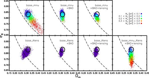
Constraints in the σ8–Ωm plane extracted from different sets of Planck Collaboration XIII (2016) Markov Chains. Top left: the case of a standard six parameter ΛCDM model (base) + a single parameter characterizing the summed mass of neutrinos (mnu) where only primary CMB (Planck TT+lowTEB) is used to constrain the model. Top middle: adopts the same model and uses the same CMB data, but also adds external BAO constraints. Top right: adds further constraints from modelling of the Planck CMB lensing power spectrum. In all of these cases ALens is fixed to unity. In the three leftmost panels in the bottom row, ALens can vary, while the summed mass of neutrinos is fixed to 0.06 eV (i.e. the minimum allowed by oscillation experiments). These three panels mirror those in the top row in terms of the data sets used to constrain the cosmological parameters. Bottom right: both ALens and Mν can vary. In all panels, the black circular and black dashed curves have the same meaning as in Fig. 1. The dots represent randomly extracted parameter sets from the Markov Chains (taking into account their weighting) and are coloured by the summed mass of neutrinos, Mν, for cases where this parameter can vary. The constraints on σ8–Ωm and on Mν depend strongly one whether one includes external data sets (particularly BAO) and on whether the lensing amplitude scale factor, ALens, is fixed or marginalized over.
Focusing on the top left panel, we see that a wide range of Mν values are allowed by the Planck primary CMB data. Furthermore, the constraints on the σ8–Ωm plane are much weaker in comparison to the case where Mν is fixed to the minimum value of 0.06 eV (compare coloured dots to the solid black contour). However, as noted previously by MacCrann et al. (2015) (see also Joudaki et al. 2017b), allowing Mν to vary does not bring the CMB constraints on σ8–Ωm into significantly better agreement with those of LSS, as the degeneracies from the two sets of constraints run approximately parallel to one another (compare the coloured dots to the dashed curve). Furthermore, as noted by Planck Collaboration XIII (2016), higher values of Mν generally result in lower values of H0 (not shown), in order to preserve the angular scale of the CMB acoustic peaks, thereby increasing the previously mentioned tension with local H0 determinations.
The inclusion of external constraints from BAO observations (top middle panel of Fig. 2) greatly reduces the allowed range of Mν, while also pegging the σ8–Ωm constraints back close to those derived from the standard model with Mν = 0.06 eV held fixed (compare coloured dots to solid black contour). It is important to note that the addition of BAO data also strongly constrains H0, to 67 ± 1 km s−1.
The further introduction of external constraints based on the modelling of the observed CMB lensing power spectrum (top right panel) does not allow for significantly higher summed neutrino masses, but it does result in a downward ≈1σ shift in σ8. That the constraints shift down slightly is not surprising, as we have already noted that the analysis of the CMB lensing power spectrum alone leads to a σ8–Ωm relation that is lower in amplitude than preferred by the primary CMB (Planck Collaboration XV 2016; see also bottom right panel of Fig. 1). It is interesting to note that the primary effect of incorporating the CMB lensing constraints is a downward shift in σ8 only, whereas it might have been anticipated that there would be a shift in both σ8 and Ωm, given the degeneracy between these two quantities for CMB lensing (Fig. 1). However, opposing constraints from the external BAO data sets strongly pin down the values of Ωm and H0 (not shown), while placing no direct constraints on σ8. The combination of BAO and CMB lensing therefore helps to break the σ8–Ωm degeneracy in the CMB lensing constraints.
In all the cases considered above, the lensing amplitude ALens was held fixed to unity when modelling the primary CMB TT data. In the three leftmost panels of the bottom row in Fig. 2, we consider the case where ALens is enabled to vary, while the summed neutrino mass is held fixed to 0.06 eV, mirroring the data sets used in the three panels in the top row. Here, we see that marginalizing over ALens results in a preference for lower values of Ωm and σ8. When BAO constraints are included, the main effect of marginalizing over ALens is a downward shift in σ8. Comparing these constraints to those derived from LSS in Fig. 1, it is clear that allowing ALens to vary already goes a good distance towards resolving the overall tension between the primary CMB and LSS and completely resolves it for some specific cases (e.g. DES Y1 and CMB lensing constraints), although it should be borne in mind that many of the constraints in Fig. 1 do not include potentially important baryonic effects.
While allowing ALens to vary does reduce the tension, it does not completely remove it for the case where the summed neutrino mass is held mixed at the minimum value allowed by oscillation experiments. Furthermore, since there is no strong a priori reason why the summed mass of neutrinos should be the minimum value, this parameter should be enabled to vary and to be constrained by astrophysical experiments. In the bottom right panel of Fig. 2, we therefore show the constraints on Mν and σ8–Ωm when ALens is marginalized over (i.e. both Mν and ALens are enabled to vary). Interestingly, while Ωm is still well determined (due to the addition of BAO), the constraints on σ8 and Mν are significantly broader compared to the case where ALens is fixed to unity. Thus, if one takes into account the apparent residual systematics remaining in the high-multipole primary CMB data, by marginalizing over ALens, massive neutrinos may potentially provide a full reconciliation of the primary CMB and LSS data sets. We say ‘may’ as it has yet to be demonstrated that current LSS cosmological constraints (e.g. those described in Fig. 1) are robust to the modifications induced by baryonic physics, such as AGN feedback. This is far from clear at present and is one of the main issues that we seek to address with BAHAMAS.
With regard to the recent constraints on Mν using measurements of the Lyman-alpha forest power spectrum by Palanque-Delabrouille et al. (2015) and Yèche et al. (2017), we first point out that the Lyman-alpha forest alone only constrains |$M_\nu \lesssim 1$| eV. The strong upper limits placed on Mν in these studies (Mν < 0.12 eV) come from the combination with the Planck primary CMB data. Both of the studies mentioned above use the fiducial Planck CMB Markov chains which adopt ALens = 1, finding an upper limit on the summed neutrino mass that is only just above the minimum value allowed by neutrino oscillation experiments. We speculate that if the Lyman-alpha forest measurements were instead combined with the Planck chains for the case where ALens can vary, that the derived constraints on Mν may actually be in tension with neutrino oscillation experiments. (This is just because marginalizing over ALens tends to lower the best-fitting value of σ8 from the primary CMB, which would in turn reduce the best-fitting value of Mν.) Such a tension would suggest that there are still relevant systematic errors in the Lyman-alpha forest data and/or modelling (e.g. Rogers et al. 2017).
Finally, it is worth noting that the Lyman-alpha forest constraints on the spectral index, ns, are in tension with constraints from Planck, with the Lyman-alpha forest data preferring a relatively low value of ns = 0.938 ± 0.010 (Palanque-Delabrouille et al. 2015), while the Planck CMB data constrains ns = 0.9655 ± 0.0062 (Planck Collaboration XIII 2016), representing a ≈3σ difference. This indicates that the Lyman-alpha forest data does actually prefer less small-scale power than predicted given the standard model of cosmology with primary CMB constraints. It is the shape of the Lyman-alpha power spectrum that allows one to individually constrain Mν and ns (or, alternatively, the running of spectral index, dns/dlnk). Even a subtle scale-dependent bias could have significant implications for the individual constraints on Mν, σ8, and ns.
3 SIMULATIONS
3.1 BAHAMAS
We use the BAHAMAS suite of cosmological hydrodynamical simulations to predict the various LSS diagnostics (e.g. cosmic shear, tSZ power spectrum, etc.) in the context of massive neutrino cosmologies. Here, we provide a brief summary of the simulations, including their feedback calibration strategy, but we refer the reader to M17 for further details.
The BAHAMAS suite of cosmological hydrodynamical simulations consists of 400 Mpc h−1 comoving on a side, periodic box simulations containing 2 × 10243 particles. We use 11 runs from that suite here, which vary the cosmological parameter values, including the summed mass of neutrinos, as discussed in detail in Section 3.2. The Boltzmann code CAMB4 (Lewis, Challinor & Lasenby 2000; April 2014 version) was used to compute the transfer functions and a modified version of N-GenIC to create the initial conditions, at a starting redshift of z = 127. N-GenIC has been modified by S. Bird to include second-order Lagrangian Perturbation Theory corrections and support for massive neutrinos.5 Note that when producing the initial conditions, we use the separate transfer functions computed by CAMB for each individual component (baryons, neutrinos, and CDM), whereas in most existing cosmological hydro simulations the baryons and CDM adopt the same transfer function, corresponding to the total mass-weighted function. Note also that we use the same random phases for each of the simulations, implying that comparisons between the different runs are not subject to cosmic variance complications.
The simulations were carried out with a version of the Lagrangian TreePM-SPH code gadget3 (last described in Springel 2005), which was modified to include new subgrid physics as part of the OverWhelmingly Large Simulations (OWLS) project (Schaye et al. 2010). The gravitational softening is fixed to 4 h−1 kpc (in physical coordinates below z = 3 and in comoving coordinates at higher redshifts) and the smoothed particle hydrodynamics (SPH) smoothing is done using the nearest 48 neighbours.
The simulations include subgrid prescriptions for metal-dependent radiative cooling (Wiersma, Schaye & Smith 2009), star formation (Schaye & Dalla Vecchia 2008), and stellar evolution, mass loss and chemical enrichment (Wiersma et al. 2009) from SNII and SNIa and asymptotic giant branch stars. The simulations also incorporate stellar feedback (Dalla Vecchia & Schaye 2008) and a prescription for supermassive black hole growth and AGN feedback (Booth & Schaye 2009, which is a modified version of the model originally developed by Springel, Di Matteo & Hernquist 2005).
As described in M17, we have adjusted the parameters that control the efficiencies of the stellar and AGN feedback so that the simulations reproduce the present-day galaxy stellar mass function (GSMF) for M* > 1010 M⊙ and the amplitude of the gas mass fraction−halo mass relation of groups and clusters, as inferred from high-resolution X-ray observations. (Synthetic X-ray observations of the simulations were used to make a like-with-like comparison in the latter case.) These two observables were chosen to ensure that the collapsed structures in the simulations have the correct baryon content in a global sense. The associated backreaction of the baryons on the total matter distribution should therefore also be broadly correct. M17 demonstrated that this simple calibrated model, where the efficiencies are fixed values (i.e. they do not depend on redshift, halo mass, etc.), reproduces an unprecedentedly wide range of properties of massive systems, including the various observed mappings between galaxies, hot gas, total mass, and black holes. Note that the number of parameters that dictate the overall feedback efficiency is small. In particular, we adjusted only two parameters for each of the two forms of feedback (stellar and AGN) to reproduce the GSMF and gas fractions over two orders of magnitude in mass for both diagnostics (see Section 4 for further discussion of the calibration procedure).
We point out that the parameters governing the feedback efficiencies are not recalibrated when varying the cosmological parameters away from the fiducial WMAP (Wilkinson Microwave Anisotropy Probe) 9-yr cosmology (with massless neutrinos) adopted in M17. But, as we will demonstrate in Section 4, the internal properties of collapsed structures (stellar masses, gas masses, etc.) are, to first order, insensitive to the variations in cosmology that we consider, even though the abundance of collapsed objects (and density fluctuations in general) depends relatively strongly on the adopted cosmology.
3.1.1 Remaining feedback calibration uncertainties
Although BAHAMAS arguably yields the best match of presently available simulations to observational constraints on the baryon content of massive systems, this does not imply that the problem of ‘baryon physics’ for LSS cosmology has been fully resolved. First, the observational data on which the simulation feedback parameters were calibrated is itself prone to non-negligible uncertainties. In particular, there is a large degree of intrinsic scatter in the gas fractions of observed X-ray-selected galaxy groups, and there is a danger that X-ray selection itself may bias our view of the overall hot gas content of groups (e.g. Anderson et al. 2015; Pearson et al. 2017). A second issue is that, in BAHAMAS, we have adopted a particular parametrization for the feedback modelling, which corresponds to the simplest case where the feedback efficiency parameters are fixed. However, more complicated dependencies could be adopted and may more closely represent feedback processes in nature. While our expectation is that the act of calibrating such models against the observed stellar and gas masses of massive systems will yield LSS predictions that will be very similar to those from BAHAMAS, we cannot presently quantify the level of expected differences. Ultimately, we will only be able to assess the remaining feedback calibration uncertainties on LSS predictions by comparing the results of different (calibrated) simulations. As already noted, BAHAMAS is a first attempt to calibrate the feedback for LSS cosmology.
While it may be difficult at present to assess how adopting other feedback parametrizations will affect the LSS predictions, we can provide a simple assessment of the role of observational uncertainties in the calibration. Specifically, while the local GSMF is pinned down with sufficient accuracy observationally, the same is not true for the gas fractions of groups and clusters. As the gas dominates the stars by mass, this uncertainty could propagate through to our cosmological parameter inference. We have therefore run a number of additional smaller test simulations that vary the subgrid AGN heating temperature so that the predicted gas fractions approximately span those seen in the observations, while leaving the predicted GSMF virtually unchanged. We have found that varying the AGN temperature by ±0.2 dex approximately achieves this aim and we have therefore run two additional large-volume simulations (L400N1024, WMAP9 cosmology) that vary the heating temperature at this level, which we will use to quantify the error in our LSS cosmology results due to uncertainties in the calibration data.
We show in Fig. 3 the predicted local GSMF and hot gas mass fraction–halo mass trends of the fiducial BAHAMAS model (solid blue), and the trends predicted by simulations where the AGN heating temperature is raised (‘hi AGN’ – dashed green) or lowered (‘low AGN’ – dot–dashed purple) by 0.2 dex, all in the context of a WMAP9 cosmology. Varying the heating temperature by ±0.2 dex yields predictions that effectively skirt the upper and lower bounds of the observed trend, as desired. These simulations should therefore provide us with a (hopefully) conservative estimate of the error in the calibration due to uncertainties/scatter in the observational data against which the simulations were calibrated.
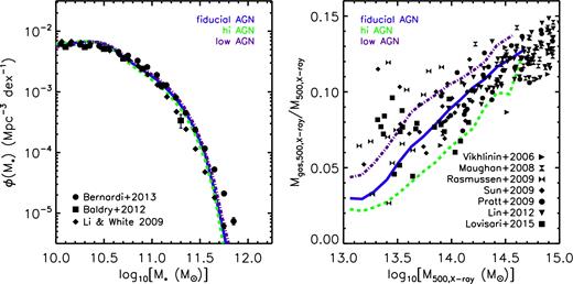
Comparison of the predicted local GSMF (left) and hot gas mass fraction–total halo mass trends (right) of the fiducial BAHAMAS model (solid blue) with that predicted by simulations where the subgrid AGN heating temperature is raised (‘hi AGN’ – dashed green) or lowered (‘low AGN’ – dot–dashed purple) by 0.2 dex, all in the context of a WMAP9 cosmology. Stellar masses in the left-hand panel are computed within a 30 kpc aperture in the simulations, while halo masses and gas fractions in the right-hand panel are derived from a synthetic X-ray analysis of a mass-limited sample (all haloes with M500, true > 1013 m⊙). See M17 for further details. The curves in the right-hand panel correspond to the median relations (the simulations predict a similar amount of intrinsic scatter as seen in the data, see Fig. 4). As shown by M17, varying the AGN heating temperature has very little effect on the GSMF but does affect the gas mass fractions. Varying the heating temperature by ±0.2 dex yields predictions that effectively skirt the upper and lower bounds of the observed trend. We will use these additional simulations to help quantify the level of error in our cosmological constraints due to imperfect feedback calibration.
While these simulations enclose the scatter in the amplitude of the observed gas fraction–halo mass relation, there is an apparent difference in the predicted and observed slopes of the relation at low mass (the galaxy group regime) that is worth commenting on. This difference is likely explained by selection effects. Specifically, for the simulations we select all haloes above a given spherical overdensity mass for analysis, whereas the X-ray constraints in Fig. 3 are generally derived from follow-up Chandra or XMM–Newton observations of group samples derived from X-ray flux-limited samples. Naively, we expect galaxy groups that are more gas rich to also be more X-ray luminous, which ought to flatten the observed relation. We note that recent stacking constraints on the relation between tSZ effect flux and halo mass (e.g. Planck Collaboration XI 2013; Wang et al. 2016; Lim et al. 2018; Jakobs et al. 2018), including its slope, are reproduced remarkably well by our simulations (e.g. M17; Lim et al. 2018; Jakobs et al. 2018), although converting the observed tSZ effect measured within the Planck beam to an estimate of the gas fraction within the halo virial radius is non-trivial (Le Brun, McCarthy & Melin 2015). Future high-resolution tSZ effect observations of optically selected groups will be invaluable for nailing down the precise form of the baryon mass–halo mass relation at low masses.
Finally, while we have only varied the feedback prescription in the context of a specific cosmology, we point out that in Mummery et al. (2017), we have shown that the effects of feedback on LSS are separable from those of massive neutrinos. Thus, it is sufficient for our purposes to propagate the uncertainties in the feedback modelling using a single cosmological model.
3.2 Massive neutrino implementation in BAHAMAS
To include the effects of massive neutrinos, both on the background expansion rate and the growth of density fluctuations, we use the semilinear algorithm developed by Ali-Haïmoud & Bird (2013) (see also Bond et al. 1980; Ma & Bertschinger 1995; Brandbyge et al. 2008; Brandbyge & Hannestad 2009; Bird, Viel & Haehnelt 2012), which we have implemented in the gadget3 code. The semilinear code computes neutrino perturbations on the fly at every time-step using a linear perturbation integrator, which is sourced from the non-linear baryons+CDM potential and added to the total gravitational force. As the neutrino power is calculated at every time-step, the dynamical responses of the neutrinos to the baryons+CDM and of the baryons+CDM to the neutrinos are mutually and self-consistently included. Note that because the integrator uses perturbation theory, the method does not account for the non-linear response of the neutrino component to itself. However, this limitation has negligible consequences for our purposes, as only a very small fraction of the neutrinos (with lower velocities than typical) are expected to collapse and the neutrinos as a whole constitute only a small fraction of the total matter density.
In the present simulations, we adopt the so-called normal neutrino hierarchy, rather than just assuming degenerate neutrino masses, as done in many previous simulation studies.
Caldwell et al. (2016) and Mummery et al. (2017) have previously used a subset of our neutrino simulations to explore the consequences of free streaming on collapsed haloes, such as their masses, velocity dispersions, density profiles, concentrations, and clustering. Here, our focus is on comparisons to LSS diagnostics, such as cosmic shear.
In addition to neutrinos, all of the BAHAMAS runs (i.e. with or without massive neutrinos) also include the effects of radiation when computing the background expansion rate. We find that this leads to a few per cent reduction in the amplitude of the present-day linear matter power spectrum compared to a simulation that only considers the evolution of dark matter and dark energy in the background expansion rate, if one does not rescale the input power by the growth rate so that the present-day power spectrum is correct.
3.3 Choice of cosmological parameter values
Large-volume hydrodynamical simulations are still sufficiently expensive that we cannot yet generate large grids of cosmologies with them. This will inevitably limit our ability to systematically explore the available parameter space associated with the standard model of cosmology, or extensions thereof, and to determine the best-fitting parameter values and their uncertainties. However, there is an emerging consensus that baryon physics plays an important role in shaping the total mass distribution even on very large scales (e.g. van Daalen et al. 2011, 2014; Velliscig et al. 2014; Schneider & Teyssier 2015) and if these effects are ignored, or modelled inaccurately, they are expected to lead to significant biases (Semboloni et al. 2011; Eifler et al. 2015; Harnois-Déraps et al. 2015). It is therefore important that, even with a relatively small range of simulated cosmologies, we make comparisons with the observations to provide an independent check of the results of less expensive (but ultimately less accurate) methods, such as those based on the halo model. But which cosmologies should we focus on?
To significantly narrow down the available cosmological parameter space, we take guidance from the two most recent all-sky CMB surveys, by the WMAP and Planck missions. In the context of the six-parameter standard ΛCDM model of cosmology, comparisons to the primary CMB alone already pin down the best-fitting parameter values to a few per cent accuracy and the model agrees every well with the CMB data. However, it must be noted that the best-fitting parameters inferred from the WMAP and Planck data are not in perfect agreement, differing in some cases at up to the 2σ level. This motivates us to consider two sets of cosmologies, one from each of the CMB missions (see Table 1). Furthermore, as the CMB is not particularly sensitive to possible ‘late-time’ effects (e.g. time-varying dark energy, massive neutrinos, dark matter interactions/decay, etc.), it remains crucially important to make comparisons to the observed evolution of the Universe, including that of LSS, to test our cosmological framework.
We adopt the following strategy when selecting the values for the various cosmological parameters. We first choose a number of values for the summed neutrino mass, Mν, that we wish to simulate. Here, we choose four different values, ranging from 0.06 up to 0.48 eV in factors of 2 (i.e. Mν = 0.06, 0.12, 0.24, and 0.48 eV). Using the Markov Chains of Planck Collaboration XIII (2016) corresponding to the bottom right panel of Fig. 2; i.e. CMB+BAO+CMB lensing with marginalization over ALens (see discussion in Section 2), we select all of the parameter sets that have summed neutrino masses within ΔMν = 0.02 of the target value. The weighted mean values for each of the other important cosmological parameters is then computed using the supplied weights of each selected parameter set in the chain. We follow this procedure for each of the summed neutrino mass cases we consider. We have verified that when selecting the parameter values in this way the predicted CMB TT angular power spectrum (computed by CAMB) is virtually indistinguishable for the four different massive neutrino cases we consider. Henceforth, we refer to the simulations whose cosmological parameter values were selected in this way as being ‘Planck2015/ALens-based’.
Prior to adopting the above strategy for the ‘Planck2015/ALens-based’ simulations, we ran a number of ‘WMAP9-based’ and ‘Planck2013-based’ simulations with massive neutrinos in which all of the cosmological parameters apart from Ωcdm (i.e. H0, Ωb, Ωm, ns, and As) were held fixed at their primary CMB maximum-likelihood values (from Hinshaw et al. 2009 and Planck Collaboration XVI 2014, respectively) assuming massless neutrinos. The CDM matter density was reduced to maintain a flat geometry, so that Ωb + Ωm + ΩΛ + Ων = 1 given the neutrino mass density of the run. The disadvantage of this strategy is that it will not precisely preserve the predicted CMB angular power spectrum, since the neutrinos are relativistic at recombination but evolve like matter (i.e. are non-relativistic) today. The deviations in the predicted power spectrum are quite small, though, given that we are only considering cases with |$\Omega _\nu \lesssim 0.01$|, and would not be easily detectable with either Planck or WMAP (as noted previously, the Planck CMB only constraint is |$M_\nu \lesssim 0.70$| eV, corresponding to |$\Omega _\nu \lesssim 0.017$|). This strategy allows one to see the effects of massive neutrinos in the absence of variations of the other parameters. For these reasons, we include the ‘WMAP9-based’ and ‘Planck2013-based’ runs in our analysis as well.
A summary of the runs used in this study is given in Table 1.
Cosmological parameter values for the simulations presented here. The columns are: (1) the summed mass of the three active neutrino species (we adopt a normal hierarchy for the individual masses); (2) Hubble's constant; (3) present-day baryon density; (4) present-day dark matter density; (5) present-day neutrino density, computed as Ων = Mν/(93.14 eV h2); (6) spectral index of the initial power spectrum; (7) amplitude of the initial matter power spectrum at a camb pivot k of 2 × 10⁻³ Mpc−1; (8) present-day (linearly evolved) amplitude of the matter power spectrum on a scale of 8 Mpc h−1 (note that we use As rather than σ8 to compute the power spectrum used for the initial conditions, thus the ICs are ‘CMB normalized’). In addition to the cosmological parameters, we also list the following simulation parameters: (9) dark matter particle mass and (10) initial baryon particle mass.
| (1) | (2) | (3) | (4) | (5) | (6) | (7) | (8) | (9) | (10) |
|---|---|---|---|---|---|---|---|---|---|
| Mν | H0 | Ωb | Ωcdm | Ων | ns | As | σ8 | MDM | Mbar, init |
| (eV) | (km s−1 Mpc−1) | (10−9) | [109 M⊙ h−1] | [108 M⊙ h−1] | |||||
| Planck2015/ALens-based | |||||||||
| 0.06 | 67.87 | 0.0482 | 0.2571 | 0.0014 | 0.9701 | 2.309 | 0.8085 | 4.25 | 7.97 |
| 0.12 | 67.68 | 0.0488 | 0.2574 | 0.0029 | 0.9693 | 2.326 | 0.7943 | 4.26 | 8.07 |
| 0.24 | 67.23 | 0.0496 | 0.2576 | 0.0057 | 0.9733 | 2.315 | 0.7664 | 4.26 | 8.21 |
| 0.48 | 66.43 | 0.0513 | 0.2567 | 0.0117 | 0.9811 | 2.253 | 0.7030 | 4.25 | 8.49 |
| Planck2013-based | |||||||||
| 0.0 | 67.11 | 0.0490 | 0.2685 | 0.0 | 0.9624 | 2.405 | 0.8341 | 4.44 | 8.11 |
| 0.24 | 67.11 | 0.0490 | 0.2628 | 0.0057 | 0.9624 | 2.405 | 0.7759 | 4.35 | 8.11 |
| WMAP9-based | |||||||||
| 0.0 | 70.00 | 0.0463 | 0.2330 | 0.0 | 0.9720 | 2.392 | 0.8211 | 3.85 | 7.66 |
| 0.06 | 70.00 | 0.0463 | 0.2317 | 0.0013 | 0.9720 | 2.392 | 0.8069 | 3.83 | 7.66 |
| 0.12 | 70.00 | 0.0463 | 0.2304 | 0.0026 | 0.9720 | 2.392 | 0.7924 | 3.81 | 7.66 |
| 0.24 | 70.00 | 0.0463 | 0.2277 | 0.0053 | 0.9720 | 2.392 | 0.7600 | 3.77 | 7.66 |
| 0.48 | 70.00 | 0.0463 | 0.2225 | 0.0105 | 0.9720 | 2.392 | 0.7001 | 3.68 | 7.66 |
3.4 Light-cones and map-making
3.4.1 Light-cones
To make like-with-like comparisons to the various LSS observations, we first construct light-cones. This is done by stacking randomly rotated and translated simulation snapshots along the line of sight (e.g. da Silva et al. 2000), back to z = 3. Each of our simulations has 15 snapshots between the present day and z = 3, output at z = 0.0, 0.125, 0.25, 0.375, 0.5, 0.75, 1.0, 1.25, 1.5, 1.75, 2.0, 2.25, 2.5, 2.75, and 3.0. Note that for a WMAP 9-yr cosmology, the comoving distance to z = 3 is ≈4600 Mpc h−1, implying that a minimum of 11 snapshots would need to be stacked along the line of sight, if the snapshots were written out at equal comoving distance intervals (of the box size). The snapshots, however, are not written out in equal comoving distance intervals, so occasionally we do not use a full snapshot, while for a handful of times we have to use a single snapshot (slightly) more than once.6
For a maximum redshift of z = 3, which was chosen to achieve convergence in the various LSS diagnostics we consider (such as the tSZ effect power spectrum), the maximum opening angle of the light-cone, given the size of the simulation box, is just slightly larger than 5° ; i.e. θmax = Lbox/χ(z = 3) where Lbox is the simulation comoving box size (400 Mpc h−1) and χ(z = 3) is the radial comoving distance to z = 3. We therefore create light-cones of 5 × 5 deg2 (Note that in comoving space, light rays follow straight lines, making the selection of particles and haloes falling within the light-cone a trivial task.) We produce 25 such light-cones per simulation, using different (randomly selected) rotations/translations. We use the same 25 randomly selected viewing angles for all the simulations, so that cosmic variance does not play a role when comparing them.
We have tested our light-cone algorithm on smaller box simulations, varying both the number of snapshots that are output and used in the construction of the cones as well as the maximum redshift of the cones. For all of the tests we consider here, we find that our theoretical predictions (e.g. the predicted Cℓ's for the tSZ effect power spectrum) do not change by more than a few per cent when we vary the number of snapshots used in the light-cones and maximum redshift of the light-cones away from the fiducial values of 15 and z = 3, respectively.
3.4.2 tSZ effect maps
The total contribution to the Compton y parameter in a pixel by a given particle is obtained by dividing ϒ by the physical area of the pixel at the angular diameter distance of the particle from the observer; i.e. |$y \equiv \Upsilon /L_{\rm pix}^2$|. We adopt an angular pixel size of 10 arcsec, which is generally better than what can be achieved with current tSZ telescopes.
Finally, we map the gas particles to the 2D grid using a simple ‘nearest grid point’ algorithm and integrate (sum) the y parameters of all of the gas particles along the line of sight to produce images. As in McCarthy et al. (2014), we have also produced SPH-smoothed y maps (using the angular extent of the particle's 3D smoothing length as the angular smoothing length) for comparison with our default nearest grid method. We find virtually identical results, in terms of cosmological parameter constraints, for the two approaches for mapping particles to pixels.
3.4.3 Weak-lensing convergence and shear maps
The lensing of images of background sources (e.g. galaxies and CMB temperature fluctuations) by intervening matter (LSS in this case) depends, to first order, on three quantities: the convergence κ and two (reduced) shear components, g1 and g2.
In the case of a single source plane, where ns(z) can be represented by a Dirac delta function, s(z) reduces simply to s(z) = χ(z)[1 − χ(z)/χ(zs)], where χ(z) and χ(zs) are the comoving distances to the lens and source, respectively. This is an excellent approximation for CMB lensing, where zs ≈ 1100 (i.e. last scattering surface), but it is not a good approximation for most galaxy weak-lensing surveys, which typically use samples of galaxies that span wide ranges in redshift. One therefore must use the source redshift distribution function for each individual survey to make comparisons between theory and a particular survey. When comparing to different surveys in Section 5.2, we will specify the particular forms of ns(z) that we adopt.
To evaluate equations (5) and (6) for a given light-cone, we first break the light-cone up into a number of segments along the line of sight. By default, we adopt a fixed segment width of Δz = 0.05, which we note is similar to the resolution in ns(z) adopted in current imaging surveys (e.g. KiDS and DES). We therefore have N = 60 such segments between z = 0 and zmax = 3, for which we calculate the mid-plane distances/redshifts and widths in comoving distance (i.e. χ, z, and Δχ). We evaluate the 2D overdensity at the mid-plane for each segment by collapsing each segment along the line of sight; i.e. integrating the total mass7 (due to dark matter, gas, stars, and neutrinos) to produce a surface mass density map, Σ(θ), from which we can evaluate the overdensity. The 2D overdensity map, δ(θ), is defined as |$\delta (\theta )\equiv [\Sigma (\theta )-\bar{\Sigma }]/\bar{\Sigma }$| and we evaluate |$\bar{\Sigma }$| analytically8 given Ωm of the simulation and the width of the segment, dχ.
Equations (7) and (8) are strictly valid only for the case of small deflection angles, i.e. photons travelling in straight lines in comoving coordinates. However, this so-called Born approximation has been shown previously to be very accurate in the case of weak lensing (Schneider et al. 1998; White & Vale 2004), which is our focus here.
Using the above methodology, what we calculate is the true convergence and shear fields for the simulations. However, observations cannot necessarily perfectly recover these true quantities. Leaving aside important observational challenges such as measuring unbiased galaxy shapes and estimating accurate redshifts from photometric data, there is also the potential physical issue of intrinsic alignments (IAs). That is, to recover the shear field in data one must average together many galaxies to beat down the noise, with the implicit assumption that, in the absence of lensing, there should be no preferential alignment between the galaxy orientations. If there is a preferential alignment (as might naively be expected from tidal torque theory, if galaxies inhabit the same large-scale environment), this will lead to a bias in the recovered lensing signal. In principle, we could address this issue by self-consistently lensing the simulated galaxies in our cosmological volumes. However, this is generally not possible with current large-volume simulations like BAHAMAS, since the resolution is too low to accurately predict and measure simulated galaxy shapes. One can instead assume a simple physical model of IAs (e.g. Bridle & King 2007) and marginalize over its free parameters when analysing the data, as is typically done in current studies. For this study, we neglect the effects of IAs in our modelling. We note that current observational constraints suggest that its effects are minor; e.g. by neglecting it, the observational constraints on S8 change by less than 1σ and do not reconcile the aforementioned CMB–LSS tension (e.g. Hildebrandt et al. 2017). In addition, using the high-resolution EAGLE cosmological hydrodynamical simulations, Velliscig et al. (2015) have shown that the IAs of galaxies is far weaker than that of dark matter haloes (which has, to date, been the basis of simple physical models of IAs), particularly if one selects the stars in an observationally motivated manner.
4 HOW DEGENERATE IS COSMOLOGY WITH BARYON PHYSICS?
BAHAMAS is a first attempt to explicitly calibrate the feedback in large-volume cosmological hydrodynamical simulations in order to minimize the impact of uncertain baryon physics on cosmological studies using LSS. However, an important question is: to what extent is the calibration of the feedback model parameters dependent upon cosmology? If the calibration scheme depends significantly upon cosmology, the implication is that the feedback model parameters would need to be readjusted for each cosmological model that we simulate. This would obviously complicate the cosmological analysis but may ultimately be necessary.
It is clear that if the feedback model were to be calibrated on the same observational diagnostics that are being used to infer cosmological parameter values (e.g. tSZ effect, cosmic shear, etc.), one should naturally expect there to be degeneracies between the cosmology and feedback parameters. Recognizing this, with BAHAMAS, we elected instead to calibrate the feedback on internal halo properties (specifically their stellar and baryon fractions), rather than on the abundance of haloes or the power spectrum of density fluctuations. The internal properties of haloes ought to be much less sensitive to cosmology, as processes such as violent relaxation, phase mixing, and shock heating will effectively randomize the energies of the dark matter, stars, and gas, thus mostly, though not completely9 removing their memory of the background cosmology. Another important advantage of using the baryon fractions of collapsed haloes is that it provides a direct measure of the effects of expulsive feedback: there are no known forces/processes within the standard model of cosmology other than feedback that can remove a significant fraction of the baryons from collapsed systems.10
We refer the reader to M17 for the details of the calibration procedure but, briefly, it proceeds as follows. We first adjusted the stellar feedback wind velocity to reproduce the observed abundance of M* (∼1010 M⊙) galaxies, which is the minimum mass we can resolve at the fiducial resolution. A wind velocity of ≈300 km s−1 achieves this for the fiducial resolution. (The stellar feedback mass-loading parameter also affects the abundance of low-mass galaxies, although less so than the wind velocity. We held the mass-loading parameter fixed at a value of 2.) Without AGN feedback, the simulations produce far too many massive galaxies; i.e. the well-known overcooling problem. Adopting the AGN feedback model of Booth & Schaye (2009), however, results in a strong quenching of star formation in the most massive galaxies and the resulting GSMF, which agrees well with the observations, and is relatively insensitive to the details of the AGN feedback modelling due to its self-regulating behaviour. However, the hot gas fractions and thermodynamic profiles of groups and clusters are strongly sensitive to the AGN subgrid heating temperature. We therefore adjusted the subgrid heating temperature to reproduce the amplitude of the observed local gas mass–total halo mass relation. This adjustment had no adverse effects on the GSMF. Note that we calibrated the model on the GSMF and the group/cluster gas fractions only and did not even examine (let alone calibrate on) other observables. We then subsequently demonstrated that the simulations reproduce a wide range of independent observations, including the profiles and redshift evolution of the gas and stellar content of massive systems (see also Barnes et al. 2017). This was done in M17 in the context of a WMAP9 cosmology with massless neutrinos.
Returning to this study and the possible cosmology dependence of the calibration scheme, we explicitly verified using small test runs (100 Mpc h−1 on a side boxes) that the stellar and gaseous properties of haloes in the simulations are insensitive to the variations in cosmology we are considering to the required accuracy. We therefore directly proceeded to run the large-volume (400 Mpc h−1 on a side) boxes necessary for the LSS tests without changing any aspect of the subgrid physics (feedback or otherwise). In Fig. 4, we show the resulting GSMFs and gas fraction–halo mass relations for the 11 different cosmologies that we consider here. As in M17, the stellar masses of simulated galaxies are computed within a 30 kpc (physical) aperture, which approximately mimics what is derived observationally for standard pipeline analysis in SDSS and GAMA (see the appendix of M17 for details). The halo masses and gas fractions of the simulated groups and clusters in the right-hand panel are derived by performing a synthetic X-ray analysis, as described in M17 (see also Le Brun et al. 2014).
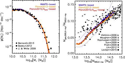
The calibrated local GSMF and hot gas mass fraction–total halo mass trends, extracted from the 11 different cosmologies considered here (see Table 1) using the same (fiducial) feedback model. Stellar masses in the left-hand panel are computed within a 30 kpc aperture in the simulations, while halo masses and gas fractions in the right-hand panel are derived from a synthetic X-ray analysis of a mass-limited sample (all haloes with M500,true > 1013 m⊙). See M17 for further details. The solid curves in the right-hand panel represent the median relation, while the dotted red curves enclose the central 68 per cent of the simulated population for the WMAP9 cosmology with massless neutrinos. The feedback model, which was calibrated in M17 using simulations run only with the WMAP9 cosmology (with massless neutrinos), produces nearly identical GSMFs and gas fractions for the other cosmologies we include here, implying that there is a negligible degree of degeneracy between cosmology and feedback, at least for the variations in cosmology that we consider here.
The resulting GSMFs and gas fraction–halo mass relations are remarkably similar. In detail, very small differences are present at the low-stellar mass end of the GSMF, which we attribute to slight differences in the resolution of the simulations (compare the particle masses in Table 1), rather than to changes in cosmology. Very small differences (typically a few per cent) are also present in the predicted gas fractions at the high-halo mass end, in the sense that the WMAP9-based simulations predict a slightly higher gas fraction compared to the Planck2013- and Planck2015/ALens-based simulations. We attribute this difference to the slightly higher universal baryon fraction, Ωb/Ωm, in the WMAP9-based cosmologies with respect to the Planck-based cosmologies. However, this difference is clearly very small compared to the scatter in the observed gas fractions of groups and clusters. Furthermore, we will demonstrate later, using the two additional runs which vary the AGN feedback (see Section 3.1.1) and alter the gas fractions by a much larger amount, that our cosmological inferences are negligibly affected by the small differences in the gas fractions of the different simulations.
On the basis of the above, we therefore conclude that our feedback calibration method is sufficiently insensitive to cosmology; i.e. there is no significant degeneracy between uncertainties in the feedback model parameters and the cosmological parameters for the variations in cosmology we consider here (see also Mummery et al. 2017). We emphasize, however, that this insensitivity to cosmology may not hold for much larger variations in the cosmological parameters or for more significant extensions to the standard model of cosmology (e.g. modified gravity). This should be tested on a case-by-case basis.
5 RESULTS
In this section, we present our constraints on the summed mass of neutrinos, Mν, derived from various statistical measures of the tSZ effect, cosmic shear, and CMB lensing.
5.1 tSZ effect
5.1.1 Angular power spectrum
In Fig. 5, we compare the predicted and observed tSZ effect angular power spectra. We focus on multipoles of ℓ > 100, which are accessible with the simulated light-cones.
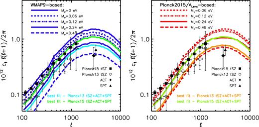
Comparison of the observed (data points with 1σ errors) and predicted (curves) tSZ effect (Compton y) angular power spectra. Left: comparison to the WMAP9-based simulations. Right: comparison to the Planck2015/ALens-based simulations. The constraints of Mν depend strongly on the adopted observational data set. Both the ACT and SPT measurements at ℓ ≈ 3000 are of significantly lower amplitude than expected for a model with minimal neutrino mass, as are the (larger-scale) Planck 2013 tSZ measurements. All three are consistent with a summed neutrino mass of ≈0.3(0.4) in the context of the WMAP9-based (Planck2015/ALens-based) simulations. However, the more recent Planck 2015 tSZ measurements are consistent with the minimal neutrino mass. See Table 2. The origin of this difference is unclear, but is probably related to residual foreground contamination (e.g. the CIB) in the tSZ effect maps (see the text for discussion).
For the observations, we use recent measurements from the South Pole Telescope (SPT, George et al. 2015) and the ACT (Sievers et al. 2013), as well as from the Planck 2013 and 2015 data releases (Planck Collaboration XXI 2014; Planck Collaboration XXII 2016). The SPT and ACT place independent constraints on the power spectrum at ℓ ∼ 3000 and are consistent with each other. However, there is a clear difference between the reported 2013 and 2015 Planck power spectra at |$\ell \lesssim 1000$|, in that the amplitude of the 2015 power spectrum is systematically higher than that of the 2013 power spectrum. The published uncertainties, which are dominated by systematic foreground subtraction uncertainties (due to point sources and the clustered infrared background, CIB), are also larger for the 2015 measurements. The larger error bars for the 2015 data set reflect a more conservative analysis of the foreground uncertainties (Comis, private communication), but the origin of the shift between the 2015 and 2013 power spectra at |$\ell \gtrsim 100$|, or even its presence, was not acknowledged or discussed by Planck Collaboration XXII (2016). For this reason, we examine the constraints using both data sets (independently).
To place constraints on the summed mass of neutrinos, we first compute the mean tSZ effect power spectrum for each of the simulations, by averaging over the power spectra computed for the 25 light-cones for each simulation. We have produced a simple function that will interpolate (or extrapolate if necessary) from these pre-computed power spectra the value of Cℓ at a specified multipole given a choice of summed neutrino mass. The interpolator fits a power law of the form Cℓ = A(1 − fν)B, where fν ≡ Ων/Ωm and A and B are constants determined by fitting the trend between Cℓ and fν at fixed ℓ from the pre-computed spectra. This is done either in the context of the WMAP9-based simulations or the Planck2015/ALens-based simulations. To determine the best-fitting neutrino mass and its uncertainty, we use the mpfit package,11 which uses the Levenberg–Marquardt technique to quickly solve the least-squares problem. Note that, as no covariance matrices were published in the tSZ observational studies, we neglect any correlation between the different multipole bins. Planck Collaboration XXI (2014) and Planck Collaboration XXII (2016) state that they have adopted a multipole binning scheme designed to minimize the covariance between the bins. If there is residual covariance remaining then our analysis will underestimate the statistical uncertainties in the derived value of Mν.
Note that when fitting the models to the data, we neglect the uncertainty in the theoretical predictions. This is because we find that, for a given simulation, the error on the calculated mean power spectrum (estimated by dividing the scatter about the mean from different sightlines by the square root of the number of sightlines) is generally considerably smaller than the observational measurement errors.12 For comparisons to future surveys, however, a more careful treatment of simulation statistical errors will be required.
It is clear from Fig. 5 that the constraints on Mν will be sensitive to both the choice of simulations (WMAP9-based versus Planck2015/ALens-based) and the observational data sets that are employed. The former is of course expected, given that the other relevant cosmological parameters (e.g. Ωm, H0, and As) differ for the two sets of simulations (owing to differences in the best-fitting parameters derived from the Planck and WMAP primary CMB data). The latter (i.e. the choice of tSZ data set) is, however, more worrying and it is clear that the inferred value of Mν will be strongly dependent upon this choice.
In Table 2, we present the constraints on Mν from the tSZ power spectrum analysis. Using Planck 2013 tSZ data, with or without additional ACT and SPT constraints, leads to a strong preference for a non-minimal neutrino mass, with a best fit of Mν ≈ 0.3(0.4) eV when using the WMAP9-based (Planck2015/ALens-based) simulations. The quality of the fits are very good in the context of either Planck 2013 tSZ data alone or in combination with ACT and SPT data, indicating approximate consistency between the Planck 2013 and ACT/SPT data. These results are consistent with the previous findings of McCarthy et al. (2014), who showed using the cosmo-OWLS simulations that the predicted tSZ effect power spectrum for a Planck 2013 cosmology was of significantly higher amplitude than the Planck 2013 and ACT/SPT power spectrum measurements.
Constraints on the summed mass of neutrinos derived from the tSZ effect power spectrum. The columns are: (1) observational data set used; (2) best-fitting value of Mν (eV) with 1σ uncertainty; and (3) the reduced χ2 of the best fit. We have separated the constraints into two sections, based on whether the WMAP9-based or Planck2015/ALens-based simulations were used for the theoretical modelling.
| (1) | (2) | (3) |
|---|---|---|
| Data set | Mν (eV) | χ2/d.o.f. |
| Planck2015/ALens-based | ||
| Planck2013+SPT+ACT | 0.43 ± 0.04 | 0.80 |
| Planck2015+SPT+ACT | 0.24 ± 0.03 | 3.64 |
| Planck2013 tSZ only | 0.37 ± 0.05 | 0.57 |
| Planck2015 tSZ only | 0.07 ± 0.03 | 0.60 |
| WMAP9-based | ||
| Planck2013+SPT+ACT | 0.31 ± 0.04 | 0.76 |
| Planck2015+SPT+ACT | 0.15 ± 0.03 | 3.30 |
| Planck2013 tSZ only | 0.27 ± 0.04 | 0.54 |
| Planck2015 tSZ only | 0.02 ± 0.02 | 0.45 |
When fitting to Planck 2015 tSZ data only (not shown), however, the picture changes significantly, with a preference for a minimal contribution from massive neutrinos (see Table 2). The quality of the fit in this case is also good (i.e. the standard model is a good fit). This is consistent with the recent findings of Dolag, Komatsu & Sunyaev (2016), who compared the results of their Magneticum simulations (which were scaled to a Planck 2015 cosmology with minimal neutrino mass) to the Planck 2015 tSZ data and also found relatively good agreement. However, we note that the Planck 2015 tSZ data is in apparent conflict with the SPT and ACT constraints, as a simultaneous fit to all three data sets leads to a poor reduced χ2. This statement assumes that the simulated tSZ power spectra have approximately the correct shape.
Given that the tSZ effect is probing baryons, it is interesting to ask how sensitive the constraints are to uncertainties in the feedback modelling. A related question is, can these uncertainties accommodate the apparent conflict (in amplitude) between the Planck 2015 tSZ measurements and the ACT and SPT measurements? To address these questions, we show in Fig. 6, the effects of varying the importance of the AGN feedback, as described in Section 3.1.1. (This is done in the context of a WMAP9 cosmology with massless neutrinos.) Note that the AGN variations bracket the observed gas fractions of groups and clusters (see Fig. 3). From this comparison, we conclude that the tSZ power spectrum is virtually insensitive to feedback modelling uncertainties on large scales, corresponding to multipoles of |$\ell \lesssim 500$| or so (see also Komatsu & Kitayama 1999; Battaglia et al. 2010; McCarthy et al. 2014). At smaller scales, the modelling uncertainties become more significant, but we find that they are insufficiently large to reconcile the Planck 2015 tSZ measurements with the ACT and SPT measurements. We therefore conclude that uncertainties in the feedback modelling do not make the case for massive neutrinos any more or less compelling.
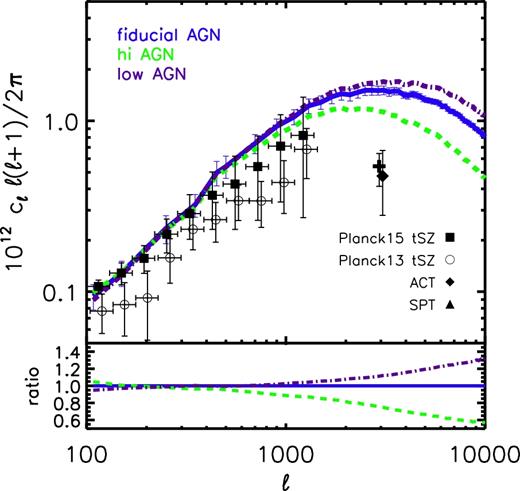
The sensitivity of the predicted tSZ effect power spectrum to uncertainties in feedback modelling, in the context of the WMAP9-based cosmology with massless neutrinos. We compare the fiducial BAHAMAS model with two runs which vary the AGN feedback (see Fig. 3). The angular power spectrum is insensitive to baryon physics at |$\ell \lesssim 500$| but can vary at the tens of percent level on scales of a few arcminutes and smaller (|$\ell \gtrsim 3000$|). Note that the uncertainties are not sufficiently large to reconcile the differing constraints on Mν derived from the Planck 2015 data and ACT and SPT data.
It is clear that, at present, systematic errors in the measurements of the power spectrum associated with foreground contamination, particularly at large scales, are the main impediment to arriving at a robust constraint on Mν from the tSZ effect power spectrum.13
5.1.2 One-point probability distribution function
The tSZ effect signal on the sky is not a Gaussian random field and is therefore not fully described by the two-point angular power spectrum. Recognizing this, previous studies have examined what cosmological constraints can be obtained by looking at other moments of the tSZ signal, including the one-point PDF and the tSZ bispectrum (e.g. Wilson et al. 2012; Hill et al. 2014; Planck Collaboration XXI 2014). Here, we compare Planck measurements of the one-point PDF (Planck Collaboration XXII 2016, we use the Planck NILC map) to that derived from the BAHAMAS simulations. We plan to examine the bispectrum and other higher order statistics in future work.
In Fig. 7, we compare the predicted and observed one-point PDFs, defined as P(y) = Npix(y)/(dydΩ), where dΩ is the solid angle in deg2. The one-point PDF just describes the frequency of pixels (per solid angle) as a function of the Compton y; i.e. it is derived by making a histogram of the y values. To derive the simulated one-point PDFs, we do the following. We first rebin the simulated Compton y maps so that the pixels are of the same size as the Planck map. The Planck map is in healpix format with Nside = 2048 resolution, corresponding to a pixel length of θpix ≈ 1.72 arcmin. Therefore, the simulated maps must be degraded by approximately a factor of 10. We then convolve the simulated maps with a Gaussian kernel with a full width at half-maximum of 10 arcmin, as was done in the construction of the Plancky map. (Note that this was not necessary for the angular power spectrum analysis in Section 5.1.1, as the beam was deconvolved when computing the observed power spectrum, but it has not been deconvolved for the observed one-point PDF analysis.) To minimize the impact of noise, Planck Collaboration XXII (2016) further filtered their y map in harmonic space in order to emphasize the multipole range where the tSZ signal is large compared to the instrumental noise. We apply the same filtering scheme to our simulated y maps using the Planck filter (kindly provided by B. Comis), which we do in Fourier space rather than harmonic space, adopting the flat-sky approximation |$\ell \approx 2 \pi u$|, where u is the angular Fourier wavenumber . We then add realistic noise to our maps, by randomly sampling from the observed PDF (post-filtering) derived from the Planck map after all of the detected tSZ sources have been masked (see the dotted curves in Fig. 7). (The PDF of this masked Plancky map is consistent with being entirely due to noise and imperfect contamination removal.) Finally, we compute the simulated PDF by averaging over the 25 light-cones for each simulation. Note that the 1σ error bars in Fig. 7 on the observed and simulated one-point PDFs reflect Poisson uncertainties only. However, the main uncertainty for the one-point PDF analysis is the cone-to-cone scatter in the simulations, as the high-y tail is dominated by very massive, nearby clusters (Dolag et al. 2016).
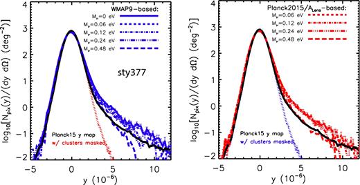
Comparison of the observed (black curve) and predicted tSZ effect (Compton y) normalized one-point PDF. Left: comparison to the WMAP9-based simulations. Right: comparison to the Planck2015/ALens-based simulations. The black data points in both panels represent the one-point PDF derived from the Planck 2015 Compton y (NILC) map. To make a like-with-like comparison, the simulated tSZ effect maps were rebinned, convolved with the Planck beam, filtered in Fourier space (as in Planck Collaboration XXII 2016), and had realistic noise/contamination added (see the text). The high y tail of the one-point PDF is sensitive to the abundance of massive clusters and therefore to the neutrino mass.
Over the range |$y \lesssim 3\times 10^{-6}$|, the one-point PDF is dominated by noise/contamination errors. We therefore follow the approach of Planck Collaboration XXII (2016) and restrict our cosmological analysis to pixels with y ≥ 4.5 × 10⁻⁶ (but note that the results are not strongly sensitive to the precise threshold). It is immediately apparent from Fig. 7 that the limited volume of the simulations results in relatively noisy predictions of the mean one-point PDF for the brightest pixels. The cone-to-cone scatter about the mean (not shown) is also significant. However, in spite of this, it is still evident that relatively high summed neutrino masses are required to reduce the overall amplitude to a level that is comparable to what is observed by Planck.
Given the relatively noisy predictions, we opt here to simply integrate the one-point PDFs above the noise limit. This yields a single value, which is the number of pixels with y ≥ 4.5 × 10⁻⁶ deg−2, for each simulation. (This statistic is analogous to tSZ cluster number counts but instead the counts involve the number of bright pixels rather than the number of massive clusters.) The Planck map yields a total of 0.877 ± 0.007 deg−2, where the uncertainty reflects Poisson errors only. The WMAP9-based simulations yield 1.822 ± 0.653, 1.482 ± 0.573, 1.224 ± 0.488, 0.939 ± 0.372, and 0.402 ± 0.209 deg−2 for the simulations with Mν = 0.0, 0.06, 0.12, 0.24, and 0.48 eV, respectively. The Planck2015/ALens-based simulations yield 1.637 ± 0.614, 1.514 ± 0.548, 1.242 ± 0.463, and 0.555 ± 0.292 deg−2 for the simulations with Mν = 0.06, 0.12, 0.24, and 0.48 eV, respectively. The quoted errors for the simulations reflect the error on the mean from the 25 light-cones, computed as the rms divided by the square root of 25. The Poisson uncertainties for the simulations are approximately an order of magnitude smaller than the error on the mean.
Using a simple interpolation scheme in analogy to that for the power spectrum analysis, we find a best-fitting neutrino mass of |$M_\nu =0.29_{-0.19}^{+0.09} (0.36_{-0.19}^{+0.11})$| eV for the WMAP9-based (Planck2015/ALens-based) simulations. These constraints are insensitive to uncertainties in the feedback modelling, as we find that the AGN variation runs only modify the predicted ‘tSZ pixel counts’ by ±5 per cent, while the error on the mean of a given simulation is typically 40 per cent.
The derived constraints on Mν are consistent with the power spectrum analysis when adopting the Planck 2013 power spectrum results and are also similar to what one would infer using ACT or SPT power spectrum data alone (see Fig. 5). On the other hand, the best-fitting Mν from the integrated one-point PDF is significantly higher than what we derive from power spectrum analysis using the Planck 2015 power spectrum data. This is interesting as the present analysis uses the same Compton y map as the Planck 2015 power spectrum analysis. The origin of this difference is unclear. It may reflect differences in the effects of remaining foreground contamination for the two tests (naively we expect the power spectrum to be more susceptible to these uncertainties).
5.2 Cosmic shear
Below we present our constraints on Mν from analysis of the lensing shape correlation functions (i.e. cosmic shear). We compare to two of the most recent cosmic shear surveys: CFHTLenS and the KiDS-450 results. Since the surveys have different galaxy selection criteria with different source redshift distributions, implying that they are probing LSS at somewhat different redshifts, we analyse these data sets independently.
We note that we have also made comparisons to the DES Science Verification cosmic shear results (Dark Energy Survey Collaboration et al. 2016), but the relatively small survey area, which leads to relatively large errors on the correlation function measurements, prevents a useful constraint on the neutrino mass. In addition, the Science Verification results have now been superseded by the DES Y1 results (Troxel et al. 2017) based on a survey area that is approximately 10 times larger. However, the DES collaboration has yet to make the Year 1 source redshift distributions and correlation function measurements publicly available. A comparison with BAHAMAS will therefore have to be deferred to a later study. We note, however, that the derived constraints in the σ8–Ωm plane from DES Y1 cosmic shear data are consistent with the KiDS-450 constraints of Hildebrandt et al. (2017, see Fig. 1).
5.2.1 Comparison to CFHTLenS
CFHTLenS is a five-band optical imaging survey conducted with the MegaCam CCD imager on the Canada–France–Hawaii Telescope (Heymans et al. 2012). The completed survey spans approximately 154 deg2. There have been three separate cosmic shear analyses of the CFHTLenS survey to date, which include the 2D (i.e. a single tomographic bin) analysis of Kilbinger et al. (2013, hereafter K13), the 3D tomographic analysis of Heymans et al. (2013, hereafter H13), and a recent update of the 3D analysis by Joudaki et al. (2017a, hereafter J17a). In terms of the shear measurements, the main difference between H13 and J17a is that the latter have extended the measurements to somewhat larger scales using a new covariance matrix calibrated with an updated set of N-body simulations. Also, J17a use seven tomographic bins spanning the redshift range 0.15 < z < 1.3, whereas H13 use six spanning 0.2 < z < 1.3. (There are also important differences in the theoretical modelling between the two studies, but this is not relevant here.)
To compute simulated shear maps suitable for comparison to these three data sets, we have retrieved the appropriate background source redshift distributions for the K13, H13, and J17a data sets from the CFHTLenS website.14 The source redshift distributions are necessary to evaluate the lensing kernel required for computing the simulated shear maps (see equations 5–8). In the present analysis, which is largely a proof of concept that hydro simulations can be used directly for cosmological analyses, we ignore the uncertainty in the photometric redshifts and do not marginalize over a potential offset factor between the estimated and true redshifts. Going forward, the aim is to directly integrate the BAHAMAS simulations (via emulators, see Section 6) into the cosmological pipelines being developed for the next generation of LSS surveys.
With shear maps in hand, we compute shear auto- (in the case of 2D) and cross-correlation (tomographic) functions using the publicly available athena tree code15 (Kilbinger, Bonnett & Coupon 2014). Given a catalogue(s) containing the angular coordinates (e.g. RA, dec.) and the complex ellipticities, athena returns estimates of the two shape correlation functions ξ±(θ) = 〈γtγt〉 ± 〈γ×γ×〉. We pass athena the simulated complex reduced shear maps, g1 and g2, which is equivalent to the complex ellipticity in the absence of shape noise. Adding realistic shape noise to the simulated shear maps would be straightforward but there is nothing to be gained by doing so, since it would only increase the error bars on the derived Mν but without shifting the estimate (i.e. shape noise does not bias the result).
In analogy to the tSZ effect analysis above, we average the correlation functions over the 25 light-cones for each simulation and we produce a function that interpolates (or extrapolates if necessary) the correlation functions for a given choice of angular scale, θ, and summed neutrino mass, Mν. We use the mpfit package, which calls the interpolator, to determine the best-fitting and 1σ errors. This analysis uses the full publicly available covariance matrices16 of each of the CFHTLenS data sets, which we downloaded from the CFHTLenS website. Note that, when fitting the data, we fit both the ξ+ and ξ− functions simultaneously, and for tomographic analyses, we fit all redshifts bins simultaneously. As discussed in Section 3.4.3, our analysis neglects IAs of background sources.
In Fig. 8, we compare the predicted shape correlation functions to the 2D measurements of K13. When fitting to the K13 data set, we use the angular scale range employed in that study, spanning 0.9–300 arcmin, with 21 angular bins for both the ξ+ and ξ− functions and their covariance matrices. The amplitude of the observed correlation functions is clearly lower than expected for either a Planck 2015 or a WMAP 9 cosmology with minimal neutrino mass. A summed neutrino mass of Mν ≈ 0.3(0.5) eV (see Table 3), however, yields relatively good agreement with the data for the WMAP9-based (Planck2015/ALens-based) simulations. With a reduced χ2 ≈ 1.4 for the best-fitting cases, the ‘goodness of fit’ to the data is reasonable, though clearly not perfect, and is similar to the quality of the fits reported in previous cosmic shear studies that use the halo model or halofit (e.g. K13, H13, J17a).
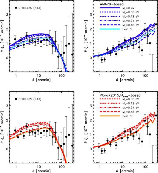
Comparison of the predicted cosmic shear shape correlation functions to the 2D CFHTLenS measurements of Kilbinger et al. (2013, data points with 1σ error bars). Left: the ξ+ correlation function, defined as ξ+(θ) = 〈γtγt〉 + 〈γ×γ×〉, where γr and γt are the radial and tangential shear components. Right: the ξ− correlation function, defined as ξ+(θ) = 〈γtγt〉 − 〈γ×γ×〉. Top: comparison using the WMAP9-based simulations. Bottom: comparison using the Planck2015/ALens-based simulations. The amplitudes of the observed correlation functions are significantly lower than expected for either a WMAP9 or Planck 2015 cosmology with minimal neutrino mass (see Table 3).
It is worth briefly commenting on the apparent negative ξ+ correlation predicted by the simulations at large angular scales (|$\theta \gtrsim 100$| arcmin). This negative correlation is a consequence of the finite box size of the simulations; i.e. it is due to a lack of large-scale k modes that are important at large angular scales (see e.g. Harnois-Déraps & van Waerbeke 2015 for a detailed discussion of this effect). For the comparisons in this study, this limitation is unimportant because these scales are generally not yet probed by tomographic (3D) analyses (see below) and are only measured with a very low signal-to-noise ratio in 2D tests, such as in the present case. We have explicitly verified that none of our cosmological results change significantly by excluding these large angular scales.
There has been much interest recently in the possible bias in cosmological constraints from cosmic shear analyses that neglect baryonic feedback (e.g. Semboloni et al. 2011; Eifler et al. 2015). This is motivated by previous simulation work, which has found that the matter power spectrum can be modified by up to ∼20–30 per cent by baryonic processes, relative to that of a dark matter-only simulation and that the difference only becomes negligible (i.e. <1 per cent) on relatively large scales of |$k\lesssim 0.3\,h$| Mpc−1 (e.g. van Daalen et al. 2011; Mummery et al. 2017). Therefore, an important question is, how sensitive are the neutrino mass constraints to uncertainties in the feedback modelling? To address this question, we show in Fig. 9, the effect of varying the strength of the AGN feedback on the predicted cosmic shear correlation functions. This is done in the context of the WMAP9-based simulation with massless neutrinos and using the CFHTLenS 2D source redshift distribution. For comparison, we also show the correlation functions predicted by a dark matter-only simulation with the same cosmology.
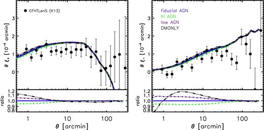
The sensitivity of the predicted cosmic shear shape correlation functions to uncertainties in feedback modelling, in the context of the WMAP9-based cosmology with massless neutrinos. The ξ+ correlation function (left-hand panel) is uncertain at the ≈5 per cent level at θ ∼ 1 arcmin and is essentially unaffected at scales of |$\theta \gtrsim 10$| arcmin. The ξ− correlation function (right-hand panel) is more sensitive to the inner regions of haloes and sizeable uncertainties persist out to 30–40 arcmin. At scales of |$\theta \lesssim 1$| arcmin, hydrodynamical simulations predict more power than a dark matter-only simulation for ξ−, likely owing to stars (e.g. brightest cluster galaxies). The uncertainty in the baryonic effects is too small to reconcile the standard model with minimal neutrino mass with the observed correlation functions.
The effects of baryon physics (and variations thereof) becomes noticeable at θ < 10 arcmin for the ξ+ correlation function and for θ < 50 arcmin for the ξ− correlation function. For example, relative to the fiducial BAHAMAS model, the ‘high AGN’ model predicts a lower value of ξ+ by ≈5 per cent at θ ≈ 1 arcmin, but is virtually identical to that of the fiducial simulation at |$\theta \gtrsim 10$| arcmin. The ‘low AGN’ model, on the other hand, has a higher value of ξ+, also by ≈5 per cent, at θ ≈ 1 arcmin, but is virtually the same as the fiducial model beyond 10 arcmin. Note, however, that the fiducial BAHAMAS model predicts a value of ξ+ that is ≈10 per cent lower than that of a dark matter-only simulation at θ ≈ 1 arcmin. For the ξ− correlation function, the effect is even larger and remains large out to θ ≈ 10 arcmin. Interestingly, for the ξ− correlation function, the hydrodynamical simulations predicted a stronger correlation (more power) on scales of |$\theta \lesssim 1$| arcmin compared to a dark matter-only simulation. This is likely due to the presence of stars (e.g. central galaxies) which begin to dominate the potential well on small physical scales. This behaviour was previously noted by Semboloni et al. (2011).
For the present analysis, the uncertainties in the feedback modelling translate into uncertainties in the predicted correlation functions that are still relatively small compared to the observational measurements errors. Going forward, however, future cosmic shear surveys, such as those to be undertaken with Euclid and LSST, will achieve much more precise estimates of the correlation functions and, therefore, much more care will need to be taken when modelling the effects of baryons, particularly in the ξ− correlation function. On the positive side, the differing dependencies of ξ+ and ξ− to cosmology and baryonic effects suggests that the cosmic shear data itself may be a useful probe of both (e.g. Semboloni, Hoekstra & Schaye 2013; Harnois-Déraps et al. 2015; Foreman, Becker & Wechsler 2016). Cross-correlation of lensing surveys with surveys of the baryons (e.g. Van Waerbeke, Hinshaw & Murray 2014; Hill & Spergel 2014; Hojjati et al. 2017) offer another interesting way to constrain both cosmology and galaxy formation physics simultaneously.
In Fig. 8, we explored what neutrino mass constraints can be obtained by using a single redshift bin. However, this does not exploit the full power of the cosmic shear surveys. One can subject the model to a more stringent test by breaking the background galaxies up into redshift (‘tomographic’) bins and performing cross-correlations between the bins. Such analyses provide additional information about the growth of LSS over cosmic time.
In Fig. 10, we compare the predicted ξ+ correlation functions from the WMAP9-based cosmology simulations with the CFHTLenS tomographic correlation functions of H13. The ξ− correlations functions for the WMAP9-based simulations and ξ± for the Planck2015/ALens-based simulations can be found in Appendix A. We adopt the same angular range cuts as employed by H13, which consist of five angular bins spanning the range from 1.5 to 30 arcmin for each of the five tomographic bins. Including all of the unique cross-correlations, the data vector contains 210 elements (summing together the ξ+ and ξ− measurements). The tomographic analysis yields best-fitting values of Mν ≈ 0.1(0.3) eV for the WMAP9-based (Planck2015/ALens-based) simulations, respectively (see Table 3). This is somewhat lower (by about 2σ) than what we obtained for the non-tomographic comparison to K13 above. The goodness of fit to the tomographic data, however, is of a similar quality to what we found for the 2D analysis above. Furthermore, we have examined the impact of uncertainties in the feedback modelling on the tomographic analysis, finding it to be subdominant to the current measurement errors.
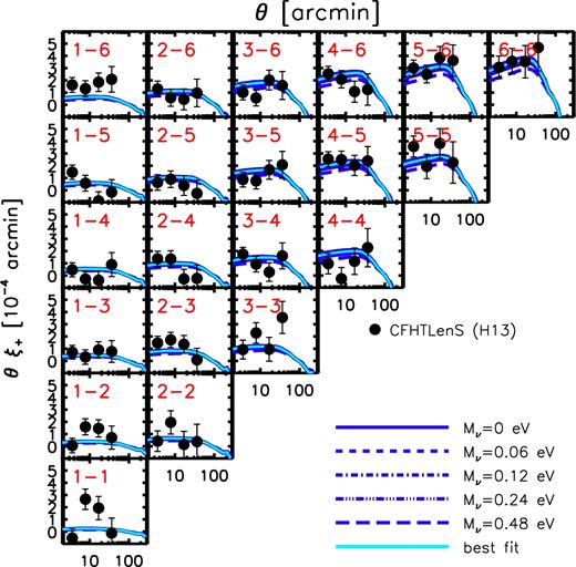
Comparison of the WMAP9-based predictions (curves) to the ξ+ tomographic CFHTLenS shear measurements of Heymans et al. (2013, data points with 1σ error bars). (The ξ− correlation functions and the comparison to the Planck2015/ALens-based simulations can be found in Appendix A.) The red numbers in each panel indicate which tomographic bins are being cross-correlated (e.g. 1–6 indicates that the first and sixth redshift bins are being cross-correlated, where the first bin correspond to the lowest redshift bin). The tomographic correlation functions also prefer a non-minimal neutrino mass, though with a somewhat smaller value than preferred by 2D (i.e. a single redshift bin) analysis – see Table 3. A comparison to a re-analysis of the tomographic CFHTLenS data by Joudaki et al. (2017a) (see the text and Appendix A) yields constraints on Mν that lie in between those derived from comparisons to the measurements of Kilbinger et al. (2013) and Heymans et al. (2013).
We note that it is the highest redshift bins (top right region of Fig. 10) in the tomographic analysis that show the strongest sensitivity to the summed neutrino mass. This just reflects the fact that photons from more distant galaxies are more strongly lensed due to intervening matter, as there is a longer path length between source and observer. It also means that any differences between the simulations are amplified, as the differences accumulate over the longer path length.
We have also made a comparison to the recent re-analysis of CFHTLenS data17 by J17a (correlation functions can be found in Appendix A). Again, we adopt the same angular range cuts as employed in the observational analysis, resulting in a data vector consisting of 280 elements. Our analysis yields constraints that lie between those obtained by comparison to K13 and H13: we find Mν ≈ 0.2(0.4) eV for the WMAP9-based (Planck2015/ALens-based) simulations, respectively (see Table 3). Here, the quality of the fit to the data is worse than for the previous cases. This was also found by J17a when comparing their models to the data, which they ascribed to a more accurately determined covariance matrix in J17a compared to that used in H13.
Overall, therefore, the CFHTLenS cosmic shear data tend to prefer a non-minimal neutrino mass, but the constraint on Mν can vary by up to 2σ depending on which correlation functions are modelled.
5.2.2 Comparison to KiDS-450
The KiDS is an ongoing four-band imaging survey being conducted with the OmegaCAM CCD mosaic camera on the VLT Survey Telescope, with the aim of completing 1500 deg2 split into two approximately equal area regions. Here, we compare to the cosmic shear measurements of Hildebrandt et al. (2017, hereafter H17), which were derived from ≈450 deg2 of the completed imaging data . H17 split their galaxy sample into four tomographic bins spanning the range 0.1 < z < 0.9. We obtained the ‘direct calibration method’ (DIR) source redshift distributions for these bins from the KiDS website,18 along with the correlation function measurements and covariance matrices.
In Fig. 11, we compare the measured ξ+ correlation functions with the WMAP9-based simulations. The corresponding ξ− functions, along with the ξ± functions for the Planck2015/ALens-based simulations, can be found in Appendix A. Our constraints on the summed mass of neutrinos from comparison to the KiDS measurements can be found in Table 3. The comparison with the WMAP9-based (Planck2015/ALens-based) simulations prefers a best-fitting summed neutrino mass of Mν ≈ 0.3(0.5) eV. This is broadly consistent with the results obtained from comparison to the 2D CFHTLenS measurements of K13 and the revisited tomographic measurements of J17a. The quality of the fit to the KiDS data set, as judged by the reduced χ2, is very good for both the WMAP9- and Planck2015/ALens-based simulations.
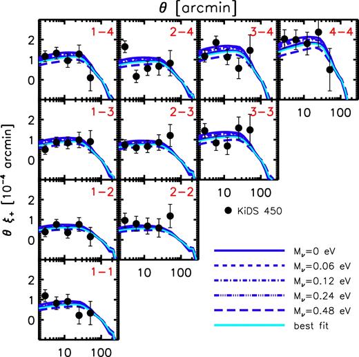
Comparison of the WMAP9-based predictions (curves)to the ξ+ tomographic KiDS-450 shear measurements of Hildebrandt et al. (2017, data points with 1σ errors). (The ξ− correlation functions and the comparison to the Planck2015/ALens-based simulations can be found in Appendix A.) The KiDS tomographic correlation functions prefer a non-minimal neutrino mass of ≈0.3(0.5) eV in the context of the WMAP9-based (Planck2015/ALens-based) simulations (see Table 3).
Constraints on the summed mass of neutrinos derived from cosmic shear (i.e. shape correlation function analysis). The columns are: (1) observational data set used; (2) best-fitting value of Mν (eV) with 1σ uncertainty; and (3) the reduced χ2 of the best fit. We have separated the constraints into two sections, based on whether the WMAP9-based or Planck2015/ALens-based simulations were used for the theoretical modelling.
| (1) | (2) | (3) |
|---|---|---|
| Data set | Mν (eV) | χ2/d.o.f. |
| Planck2015/ALens-based | ||
| CFHTLenS 2D (K13) | 0.53 ± 0.08 | 1.41 |
| CFHTLenS (H13) | 0.33 ± 0.09 | 1.35 |
| CFHTLenS rev. (J17) | 0.43 ± 0.10 | 1.74 |
| KiDS-450 (H17) | 0.52 ± 0.09 | 1.20 |
| WMAP9-based | ||
| CFHTLenS 2D (K13) | 0.32 ± 0.09 | 1.40 |
| CFHTLenS (H13) | 0.10 ± 0.08 | 1.35 |
| CFHTLenS rev. (J17) | 0.23 ± 0.11 | 1.74 |
| KiDS-450 (H17) | 0.30 ± 0.10 | 1.19 |
We note that the KiDS team have also attempted to constrain the summed mass of neutrinos using the KiDS correlation functions, in Joudaki et al. (2017b). For the theoretical modelling, they employed the halo model-based code of Mead et al. (2016), which has prescriptions for including the effects of baryon physics calibrated on the previous OWLS simulation results of van Daalen et al. (2011), as well as massive neutrinos and other extensions of the standard model of cosmology. Joudaki et al. (2017b) conclude that the KiDS data alone are fully compatible with a wide range of neutrino masses, as expected. When jointly fitting the KiDS cosmic shear data and the Planck CMB data, however, they conclude that their constraints are not competitive with the Planck+BAO joint constraints, quoting that the latter constrain Mν < 0.21 eV (Planck Collaboration XIII 2016). Here, we again point out that the quoted constraints are for the fiducial case with ALens fixed to unity and that the problem of apparent oversmoothing of the TT power spectrum at high multipoles has not been addressed. Allowing ALens to vary, the Planck+BAO data are not only compatible with higher values of Mν, they actually prefer it (see Fig. 2).
5.3 Cross-correlations
So far we have examined what constraints on Mν may be obtained from separate analyses of the tSZ effect and cosmic shear. However, one can combine these data sets to perform an additional independent test of the models, which is the cross-correlation of the tSZ effect with gravitational lensing. Note that this test is independent of the autocorrelation analyses we have already performed, since the autocorrelations only constrain the (projected) amplitudes of the hot gas and total mass, respectively, but say nothing about their spatial overlap (i.e. their relative phases). Cross-correlations are also appealing on observational grounds, since they tend to be less sensitive to residual foreground/background contaminants in the individual maps.
Cross-correlation analyses between the tSZ effect and gravitational lensing are not restricted to galaxy lensing. Recently, Planck (e.g. Planck Collaboration XV 2016), ACT (e.g. Sherwin et al. 2017), and SPT (e.g. Omori et al. 2017) have produced the first gravitational lensing maps of fluctuations in the primary CMB. The first cross-correlation measurements between CMB lensing and the tSZ effect and galaxy weak lensing have also been made and we compare BAHAMAS19 to these measurements to see what constraints may be obtained on Mν.
5.3.1 tSZ effect–galaxy weak lensing
Van Waerbeke et al. (2014) were the first to detect and measure the cross-correlation between the tSZ effect and galaxy weak lensing. They cross-correlated a custom Compton y map derived from the Planck 2013 data release with a lensing convergence map derived from the CFHTLenS survey, in configuration space. Hojjati et al. (2015) and Battaglia, Hill & Murray (2015) subsequently compared these measurements with the predictions of cosmological hydrodynamical simulations (with massless neutrinos), with both studies independently concluding that the observed signal was of lower amplitude than predicted when adopting the best-fitting Planck 2013 cosmology. More recently, Hojjati et al. (2017) measured the configuration-space and Fourier-space cross-correlations between the Planck 2015 Compton y map and galaxy weak-lensing measurements from the RCSLenS survey (Hildebrandt et al. 2016). Hojjati et al. note that, although RCSLenS is somewhat shallower than CFHTLenS, it is approximately four times larger in area than the latter, which leads to a more precise measurement of the cross-correlation and allowing the measurement to be extended to significantly larger scales. Here, we present a comparison to the Fourier-based cross-correlation measurements of Hojjati et al. (2017), noting that similar conclusions are obtained from a configuration-space analysis.
In Fig. 12, we compare the predicted tSZ–galaxy weak-lensing cross-correlations for the WMAP9-based (left-hand panel) and Planck2015/ALens-based (right-hand panel) simulations with the measurements of Hojjati et al. (2017). Note that, to make a like-with-like comparison to the observed cross-correlation, we use the RCSLenS source redshift distribution reported in Hojjati et al. (2017) to compute appropriate galaxy weak-lensing maps. Furthermore, we smooth the simulated galaxy weak-lensing convergence and tSZ effect maps with 10 arcmin Gaussian beams, as done for the observational data. This beam is not deconvolved from the reported cross-correlation, which is why the power decreases beyond ℓ ∼ 1000. Following our previous analyses, we use mpfit in conjunction with an interpolation function (that interpolates Cℓ at a given ℓ and choice of Mν) to derive the best-fitting value of Mν and the associated 1σ uncertainties. This analysis accounts for the small covariance between multipole bins in the measurements, using the covariance matrix of Hojjati et al. (2017). Consistent with Hojjati et al. (2017), we find that the Planck cosmology with minimal neutrino mass predicts a higher-than-observed amplitude for the cross-correlation. Allowing the neutrino mass to vary, we find that the data prefer a summed neutrino mass of Mν ≈ 0.26(0.13) eV when adopting the Planck2015/ALens-based (WMAP9-based) simulations (see Table 4 ). The goodness of fit to the data in both cases is excellent, with a reduced χ2 ≈ 1.
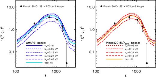
Comparison of the predicted tSZ effect–galaxy weak-lensing cross-spectrum (curves) to the measurements of Hojjati et al. (2017, data points with 1σ error bars). Left: comparison using the WMAP9-based simulations. Right: comparison using the Planck2015/ALens-based simulations. The amplitude of the observed cross-spectrum is lower than expected for either a WMAP-9yr or Planck 2015 cosmology with minimal neutrino mass. A summed neutrino mass of Mν ≈ 0.13(0.26) eV yields a good fit to the data for the WMAP9-based (Planck2015/ALens-based) simulations (see Table 4).
An interesting question is, how sensitive is tSZ–galaxy weak-lensing cross-correlation to uncertain baryon physics? Hojjati et al. (2017) explored this question using the cosmo-OWLS suite of simulations (Le Brun et al. 2014), a predecessor to BAHAMAS, finding that the cross-correlation can vary by up to a factor of 2 in amplitude at ℓ ∼ 1000. However, the models in cosmo-OWLS were not calibrated to match observational data and some of the models in the suite are inconsistent with the observed baryon fractions of groups and clusters (some lie well above the observed relation, while others lie below it). Using the full range of models will therefore likely overestimate the impact of feedback uncertainties. We revisit this question in Fig. 13 using BAHAMAS which vary the AGN feedback efficiency so that the simulated clusters skirt the upper and lower bounds of the observed cluster gas fractions (Fig. 3). We find that on large scales, |$\ell \lesssim 500$|, the cross-correlation is insensitive to baryon physics; i.e. the effects are at the |${\lesssim}5$| per cent level. At smaller angular scales (ℓ ∼ 1000), we find that the ‘hi AGN’ model predicts an amplitude approximately 15 per cent lower than to our fiducial model, whereas the ‘low AGN’ model predicts a ≈10 per cent higher amplitude relative to the fiducial model.
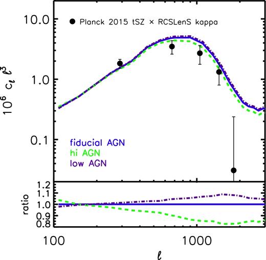
The sensitivity of the predicted tSZ effect–galaxy weak-lensing cross-spectrum to uncertainties in the feedback modelling. The predicted cross-spectrum varies by only |${\lesssim}5$| per cent on scales of |$\ell \lesssim 500$|, but can vary by up to 20 per cent at ℓ > 1000. These uncertainties are subdominant compared to the present measurement errors and cannot reconcile the standard model with a Planck 2015 cosmology with minimal neutrino mass with the observations.
We emphasize that much of the difference between the different feedback variation models at small scales has been removed as a result of the convolution with the 10 arcmin beam, suitable for a comparison with Planck data. As shown by Hojjati et al. (2017), the differences between the models would be much more significant at higher resolution. Therefore, if the goal is to probe baryon physics, cross-correlation of higher resolution tSZ effect maps (such as those obtained with SPT and ACT and their imminent successors, such as SPT-3G and Advanced ACTpol) with cosmic shear surveys offers a very promising avenue to explore.
5.3.2 tSZ effect–CMB lensing
Hill & Spergel (2014) is the only study we are aware of to date to examine the cross-correlation between the tSZ effect and CMB lensing, which they did in harmonic space. They cross-correlated a custom Compton y map derived from the Planck 2013 data release with the Planck 2013 CMB lensing map. CMB lensing measurements are currently of relatively low significance compared to those of galaxy lensing. Nevertheless, Hill & Spergel (2014) derived a competitive constraint on S8 from the tSZ–CMB lensing cross-spectrum, reporting a value of S8 that lies between the best-fitting WMAP9 and Planck 2015 values (i.e. they found no significant evidence for a tension with the primary CMB).
In Fig. 14, we compare the predicted tSZ–CMB lensing cross-correlations for the WMAP9-based (left-hand panel) and Planck2015/ALens-based (right-hand panel) simulations with the rebinned measurements of Hill & Spergel (2014, see their fig. 15). For the simulated CMB lensing maps, we adopted a single source plane at z = 1100 (see Section 3.4.3) when computing the lensing convergence maps. Note that, although Hill & Spergel (2014) smoothed their maps with a 10 arcmin Gaussian prior to analysis, they deconvolved the beam when computing the cross-correlation function. We therefore use our raw (unsmoothed) simulated maps to compute the predicted cross-correlation. We also note that Hill & Spergel (2014) actually cross-correlated a map of the lensing potential, ϕ, rather than the convergence, κ, with the tSZ effect y. In multipole space, the lensing potential and convergence are related via ϕ = 2κ/[(ℓ + 1)ℓ], so we multiply our κ–y cross-spectrum by this factor to convert to a ϕ–y cross-spectrum.
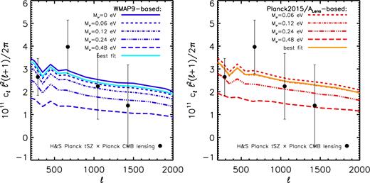
Comparison of the predicted tSZ effect–CMB lensing cross-spectrum (curves) to the measurements of Hill & Spergel (2014, data points with 1σ error bars). Left: comparison using the WMAP9-based simulations. Right: comparison using the Planck2015/ALens-based simulations. The amplitude of the observed cross-spectrum is consistent with the minimal neutrino mass case, but is also compatible with neutrino masses of up to ≈0.2(0.3) at 1σ for the WMAP9-based (Planck2015/ALens-based simulations) – see Table 4. Larger neutrino masses may also be compatible with the data if the observed cross-spectrum has some residual contamination from the CMB lensing–CIB cross-correlation, as argued by Hurier (2015).
The tSZ–CMB lensing cross-correlation data tend to prefer a low value of Mν that is consistent with the minimum neutrino mass (see Table 4). However, the measurements are still relatively noisy and can accommodate neutrino masses of up to 0.18(0.27) eV (at 1σ) when adopting WMAP9 (Planck2015) ‘priors’. The goodness of fit to the data in both the WMAP9- and Planck2015/ALens-based cases is excellent.
As discussed in Hill & Spergel (2014), the CIB is a major source of contamination for the tSZ effect–CMB lensing cross-correlation, as the CIB itself is strongly correlated with CMB lensing (Holder et al. 2013; van Engelen et al. 2015). While Hill & Spergel (2014) have taken steps to clean their maps of CIB contamination, Hurier (2015) argue that their adopted cleaning method will not completely remove it and he estimated that the amplitude of the tSZ–CMB lensing cross-correlation of Hill & Spergel (2014) may be biased high by ≈20 per cent at ℓ ∼ 1000. Applying a −20 per cent shift to the observed cross-correlation, the best-fitting value of Mν increases to 0.16 ± 0.13 (0.24 ± 0.15) eV when using the WMAP9-based (Planck2015/ALens-based) simulations, bringing it into very good agreement with the tSZ–galaxy lensing cross-correlation constraints in Section 5.3.1, but somewhat lower than preferred by the tSZ effect-only and cosmic shear-only constraints in Sections 5.1 and 5.2, respectively.
It is worth briefly commenting on why we have not applied a similar shift to the previous auto- and cross-correlations including the tSZ effect that we examined in Sections 5.1.1 and 5.3.1. The power spectra used in those analyses were derived from the Planck team's tSZ maps which were constructed using a detailed component separation algorithm that (at least in principle) accounts for CIB contamination. Hill & Spergel (2014), however, derived their own custom tSZ effect map from the Planck temperature maps (prior to the Planck 2015 data release) and used their own custom CIB cleaning methodology, which Hurier (2015) re-examined and estimated that a −20 per cent correction was required. The fact that the tSZ effect (auto-)power spectrum has changed significantly between different releases by members of the Planck team (including the new study of Bolliet et al. 2017) suggests that the issue of CIB contamination has not been fully resolved for the tSZ effect autocorrelation, but the level of remaining bias is difficult to assess. For the tSZ effect–galaxy weak-lensing cross-spectrum presented by Hojjati et al. (2017), our expectation is that CIB contamination should be minimal, since the tSZ–galaxy lensing signal is strongly weighted to low redshifts, particularly for RCSLenS data (see also Battaglia et al. 2015), whereas the CIB signal is dominated by objects at higher redshifts of |$1 \lesssim z \lesssim 5$| (e.g. Hurier 2015).
Lastly, in Fig. 15, we explore the effects of varying the AGN feedback level on the predicted tSZ–CMB lensing cross-correlation function. While there is a noticeable effect, the uncertainty in the predicted cross-correlation due to uncertainties in the feedback modelling are clearly small compared to current measurement uncertainties. This situation will likely change in the near future, as much more precise and higher resolution measurements of both the tSZ effect and CMB lensing will become available from experiments such as Advanced ACTpol. It is interesting that feedback tends to amplify the signal on large scales (low multipoles). We speculate that this is because one is typically probing the outskirts of groups and clusters at large angular scales (see e.g. the deconstruction of the tSZ effect angular power spectrum by radial ranges in Battaglia et al. 2012 and McCarthy et al. 2014) and AGN feedback tends to boost the pressure beyond the virial radius (Le Brun et al. 2015), which is a consequence of (high-redshift) gas ejection (McCarthy et al. 2011). We note that this effect is also present in the tSZ–galaxy lensing cross-correlation (see Fig. 13), but is smaller in magnitude. A detailed comparison of the deconstruction of these two cross-correlation functions into their halo mass, redshift, and radial contributions would be interesting, but we leave this for future work.
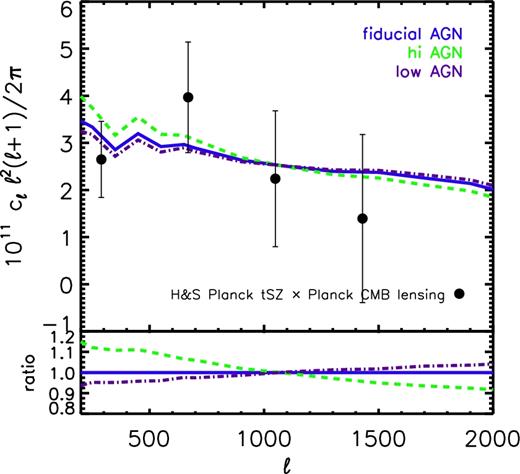
The sensitivity of the predicted tSZ effect–CMB lensing cross-spectrum to uncertainties in the feedback modelling, in the context of the WMAP9-based cosmology with massless neutrinos. The predictions vary by up to 10 per cent, depending on angular scale. Increased feedback boosts the signal on large scales, likely as a result of gas ejection (McCarthy et al. 2011). This effect is also present in the tSZ effect–galaxy lensing cross-spectrum and the tSZ effect power spectrum, though the effect there is smaller in magnitude and confined to the larger scales. The uncertainties in the feedback modelling are small compared to current measurement uncertainties but will become more relevant for future measurements from, e.g. Advanced ACTpol.
5.3.3 Galaxy lensing–CMB lensing
As a final test, to close the cross-correlation loop, we examine the cross-correlation between galaxy lensing and CMB lensing. Measurements of such lensing–lensing cross-correlations have only recently become possible, with the first detection reported by Hand et al. (2015) who cross-correlated the ACT CMB lensing map with the CS82 lensing survey. More recently, Liu & Hill (2015) cross-correlated the CFHTLenS convergence map with the Planck 2013 CMB lensing convergence map, Harnois-Déraps et al. (2016) cross-correlated the CFHTLenS and RCSLenS data with the Planck 2015 CMB lensing map, Kirk et al. (2016) cross-correlated the DES Science Verification data with the SPT CMB lensing map, Singh, Mandelbaum & Brownstein (2017) cross-correlated SDSS lensing data with the Planck 2015 CMB lensing map, and Harnois-Déraps et al. (2017) cross-correlated the KiDS-450 data with the Planck 2015 CMB lensing map. The majority of these studies reported a 1σ–2σ difference in the amplitudes of the observed cross-correlation with respect to that expected for a Planck 2015 CMB cosmology, in the sense that the observed cross-correlations were somewhat lower in amplitude than expected (i.e. consistent with the other LSS constraints we discussed in Section 2). The most sensitive measurements to date are those of Harnois-Déraps et al. (2017) and we compare to their measurements of the galaxy lensing convergence–CMB lensing convergence cross-spectra.
In Fig. 16, we compare the predicted galaxy lensing–CMB lensing cross-correlations for the WMAP9-based (left-hand panel) and Planck2015/ALens-based (right-hand panel) simulations with the measurements of Harnois-Déraps et al. (2017). (We do not use the full covariance matrices of Harnois-Déraps et al. 2017 for this analysis, only the diagonal elements, as the Fourier-based cross-correlations show little bin-to-bin covariance which can safely be ignored.) For the simulated CMB lensing maps, we adopt a single source plane at z = 1100 when computing the lensing convergence maps. For the simulations, we use the KiDS source redshift distribution spanning the full redshift range 0.1 < z < 0.9 (i.e. a single tomographic bin) to compute the predicted convergence maps. For consistency with the observational analysis of Harnois-Déraps et al. (2017), we have convolved the predicted CMB lensing maps with a 10 arcmin Gaussian but have not smoothed the simulated convergence maps.
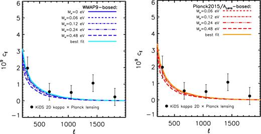
Comparison of the predicted galaxy lensing–CMB lensing cross-spectrum (curves) to the measurements of Harnois-Déraps et al. (2017, data points with 1σ error bars). Left: comparison using the WMAP9-based simulations. Right: comparison using the Planck2015/ALens-based simulations. The theoretical predictions agree well with the measurements, but current measurement errors are too large to distinguish most of the interesting neutrino mass range: the WMAP9-based comparison is compatible with |$M_\nu \lesssim 0.3$| eV, while the Planck2015/ALens-based comparison is compatible with |$M_\nu \lesssim 0.5$| eV (see Table 4).
The predicted cross-correlations agree well with the observed ones, with a best-fitting reduced χ2 ≈ 0.7 for both the WMAP9-based and Planck2015/ALens-based simulations. However, we find that the current measurement errors are too large to distinguish most of the interesting neutrino mass range: the WMAP9-based comparison is compatible with |$M_\nu \lesssim 0.3$| eV, while the Planck2015/ALens-based comparison is compatible with |$M_\nu \lesssim 0.5$| eV (see Table 4).
These constraints were derived using a single tomographic bin from KiDS. Following Harnois-Déraps et al. (2017), we have also examined what constraints can be obtained by splitting the cosmic shear data into different tomographic bins. Using the source redshift distributions of the four bins used in the observational analysis, we have computed the corresponding cosmic shear maps and cross-correlated each with the CMB lensing and then performed a joint fit to the four bins (not shown, for brevity). However, we find that this tomographic analysis does not improve the constraints on the summed neutrino mass compared to the ‘2D’ analysis above.
Finally, in Fig. 17, we explore the sensitivity of the theoretical predictions to uncertainties in the astrophysical modelling. At ℓ ∼ 1000, the uncertainty in the cross-correlation is ≈5 per cent (comparing the three AGN models). As expected, the uncertainties become somewhat larger at smaller angular scales (high multipoles), but are still only at the level of |${\sim }5{\rm -}10\,{\rm per \, cent}$|, which is smaller than current measurement errors for the CMB lensing–galaxy lensing cross-correlation. Note, however, that the differences between the fiducial BAHAMAS model and a dark matter-only simulation are quite a bit larger than this. Future high-sensitivity and high-resolution measurements of CMB lensing, combined with future cosmic shear measurements (e.g. with Euclid and LSST) may be able to distinguish effects at these levels. It is interesting to note that feedback affects the lensing-lensing cross-correlation differently than it does for CMB lensing–tSZ and cosmic shear–tSZ cross-correlations, in terms of the angular dependence (compare the bottom panels of Figs 13, 15, and 17). A joint modelling of these cross-correlations therefore offers an interesting way to constrain the feedback modelling (as well as cosmology).
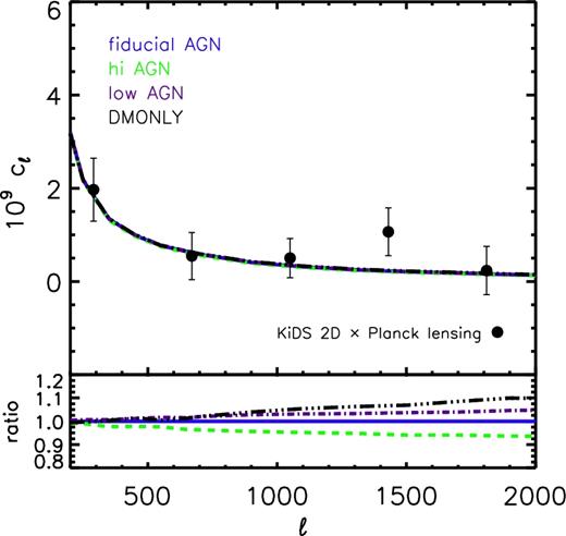
The sensitivity of the predicted galaxy lensing–CMB lensing cross-spectrum to uncertainties in the feedback modelling, in the context of the WMAP9-based cosmology with massless neutrinos. The variations are confined to a few per cent on large scales of |$\ell \lesssim 500$| but reach 5 per cent at ℓ ∼ 1000. These differences are small compared to current measurement uncertainties.
5.4 Summary of constraints
We summarize our constraints on the summed mass of neutrinos, Mν, from the comparisons to tSZ effect, cosmic shear, and CMB lensing data in Fig. 18. Note that for the Planck lensing–tSZ cross-correlation, we include a second set of constraints accounting for the CIB contamination bias estimated by Hurier (2015, see Section 5.3.3). In addition, we exclude the constraints obtained from a joint fit to the Planck 2015, ACT and SPT tSZ effect power spectrum data, as these data sets are in strong tension with each other (i.e. the joint fit is poor).
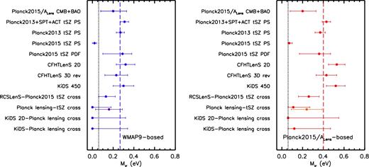
A comparison of our 1σ constraints on the summed mass of neutrinos, Mν, via the comparisons to tSZ effect, cosmic shear, and CMB lensing data. Left: constraints obtained when using the WMAP9-based simulations. Right: constraints obtained when using the Planck2015/ALens-based simulations. The vertical dotted line corresponds to the minimum value of Mν from neutrino oscillation experiments, assuming a normal hierarchy. The vertical dashed lines correspond to the best-fitting summed neutrino mass when fitting a constant to the individual constraints (excluding the discrepant Planck 2015 tSZ PS constraints). For the ‘Planck lensing–tSZ cross’ test, two sets of constraints are shown, corresponding to comparisons with the measurements of Hill & Spergel (2014) with and without taking into account possible residual CIB contamination, as suggested by Hurier (2015, see Section 5.3.3). The ‘Planck2015 CMB+BAO’ constraint in both panels corresponds to the 1σ constraint on Mν that we derive from the Planck chains with marginalization over ALens (see Section 2.1). If the CMB constraints on the other parameters originate from WMAP-9yr data, the majority of the LSS tests prefer |$M_\nu \lesssim 0.3$| eV. When adopting the Planck 2015 constraints (with marginalization over ALens) on the other parameters, the LSS tests are compatible with higher values, although there is considerable scatter in the best-fitting value of Mν between the different tests. We have shown that this scatter is likely not due to theoretical uncertainties (e.g. baryon effects). Overall, our results indicate that a non-minimal neutrino mass (i.e. Mν > 0.06 eV) is preferred, particularly if one combines the recent Planck CMB constraints with LSS.
The tests included in Fig. 18 are as follows. ‘Planck2015 CMB+BAO’ is the 1σ constraint on Mν that we derive from the Planck 2015 CMB chains with marginalization over ALens (see Section 2.1). ‘Planck2013+SPT+ACT tSZ PS’ refers to a joint fit to the Planck 2013 and SPT and ACT tSZ power spectra (see Section 5.1.1 and Table 2). ‘Planck2013 tSZ PS’ and ‘Planck2015 tSZ PS’ refer to fits to the Planck 2013 tSZ power spectrum only and to the Planck 2015 tSZ power spectrum only, respectively (see Section 5.1.1 and Table 2). ‘Planck2015 tSZ PDF’ refers to the fit to Planck 2015 tSZ one-point PDF (see Section 5.1.2). ‘CFHTLenS 2D’ and ‘CFHTLenS 3D rev’ refer to the fits to the 2D cosmic shear data of Kilbinger et al. (2013) and to the 3D tomographic data of Joudaki et al. (2017a), respectively (see Section 5.2.1 and Table 3). ‘KiDS-450’ refers to the fit to the cosmic shear tomographic data of Hildebrandt et al. (2017, see Section 5.2.2 and Table 3). ‘RCSLenS-Planck2015 tSZ cross’ refers to the fit to the RCSLenS galaxy lensing–Planck 2015 tSZ cross-spectrum measurement of Hojjati et al. (2017, see Section 5.3.1 and Table 4) (see Section 5.3.1. ‘Planck lensing-tSZ cross’ refers to the fit to the Planck 2013 CMB lensing–Planck 2013 tSZ cross-spectrum measurement of Hill & Spergel (2014, see Section 5.3.2 and Table 4). ‘KiDS 2D-Planck lensing cross’ and ‘KiDS-Planck lensing cross’ refer to the fits to the 2D and 3D (respectively) KiDS galaxy lensing–Planck 2015 CMB lensing cross-spectrum measurements of Harnois-Déraps et al. (2017, see Section 5.3.3 and Table 4).
Constraints on the summed mass of neutrinos derived from cross-correlations between the tSZ effect, CMB lensing, and cosmic shear. The columns are: (1) observational data set used; (2) best-fitting value of Mν (eV) with 1σ uncertainty; and (3) the reduced χ2 of the best fit. We have separated the constraints into two sections, based on whether the WMAP9-based or Planck2015/ALens-based simulations were used for the theoretical modelling.
| (1) | (2) | (3) |
|---|---|---|
| Data set | Mν (eV) | χ2/d.o.f. |
| Planck2015/ALens-based | ||
| RCSLenS × Planck tSZ | 0.26 ± 0.10 | 0.91 |
| Planck lensing × Planck tSZ | |$0.11_{-0.11}^{+0.16}$| | 0.51 |
| KiDS × Planck lensing | 0.12 ± 0.35 | 1.00 |
| KiDS (2D) × Planck lensing | <0.49 | 0.69 |
| WMAP9-based | ||
| RCSLenS × Planck tSZ | 0.13 ± 0.09 | 1.07 |
| Planck lensing × Planck tSZ | |$0.04_{-0.04}^{+0.14}$| | 0.47 |
| KiDS × Planck lensing | <0.34 | 1.01 |
| KiDS (2D) × Planck lensing | <0.32 | 0.73 |
When adopting CMB constraints on the other parameters from WMAP9 data (i.e. using the WMAP9-based simulations for the modelling), all of the LSS tests prefer |$M_\nu \lesssim 0.3$| eV. The tSZ effect-only (with the exception of the Planck 2015 constraints) and cosmic shear-only tests show a 2σ–3σ preference for a non-minimal neutrino mass. The various cross-correlation tests, particularly those involving CMB lensing, are compatible with these constraints but are also compatible with a minimal summed mass.
When adopting CMB constraints on the other parameters from Planck 2015 data (with marginalization over ALens, see discussion in Section 2.1), the LSS tests are compatible with masses of up to |$M_\nu \lesssim 0.5$| eV. Again, the tSZ effect-only (with the exception of the Planck 2015 tSZ power spectrum constraints) and cosmic shear-only tests show a strong preference for a non-minimal neutrino mass. The various cross-correlation tests, especially those involving CMB lensing, are not as constraining and are compatible with these tSZ-only and cosmic shear-only results but are also compatible with a minimal summed mass.
We highlight that, with the exception of the Planck 2015 tSZ power spectrum constraints, there is reasonable consistency between the different tests. Fitting a constant value of Mν to the different WMAP9-based (Planck2015/ALens-based) constraints yields a best-fitting summed neutrino mass of 0.27 ± 0.05 (0.40 ± 0.05) eV with a reduced χ2 of 0.70 (1.35), if we exclude the discrepant Planck 2015 tSZ power spectrum constraints.20 Formally speaking, our results therefore strongly support a non-minimal neutrino mass. However, our quoted uncertainties are underestimates given that we have not marginalized over the other relevant cosmological parameters (see Section 6) or observational nuisance parameters (e.g. IAs and photometric redshift errors in the case of cosmic shear). We have, however, considered the theoretical uncertainties in modelling the baryons and concluded that these are subdominant at present. We also note that the uncertainties quoted above are strongly affected by the inclusion of the Planck 2013 tSZ power spectrum constraints, but, as discussed in Section 5.1.1, there are reasons to believe that the uncertainties in the tSZ measurements are larger than quoted.
6 DISCUSSION AND CONCLUSIONS
We have used self-consistent cosmological hydrodynamical simulations from the BAHAMAS project to constrain cosmological parameters. To our knowledge, this is the first time that such simulations, as opposed to dark matter-only simulations, have been used directly to constrain cosmological parameters from LSS data. Our analysis has avoided the use of many simplifying assumptions that enter into the standard halo model-based approach (e.g. particular forms for the halo mass function and bias, parametric forms for the matter distribution within haloes, the Limber approximation, baryonic effects, etc.).
An important aspect of our study is that the physical models for stellar and AGN feedback in the simulations have been carefully calibrated to match key observational diagnostics (the GSMF and galaxy group and cluster gas fractions) so that the distribution of baryons and the backreaction of baryons on the total matter distribution are realistic. The calibration was then a posteriori checked against multiple observations of the baryon-matter connection (see M17). We have demonstrated that our calibration approach is insensitive to cosmology (see Section 4) i.e. astrophysics and variations in cosmology of interest here are not degenerate when calibrated in this way. Through the construction of light-cones and synthetic observational maps, we have been able to compare the same model to a range of different data sets (tSZ effect, cosmic shear, CMB lensing, and their various cross-correlations) that probe different aspects of the matter distribution on different scales and at different cosmic epochs. Our work demonstrates that for current data the effect of baryonic physics is significant, but that the residual uncertainties in the baryonic modelling (derived from measurement error in the calibration data) is not. This thus represents a strong proof of concept validating the use of hydrodynamical simulations for LSS cosmology.
Consistent with a number of previous LSS studies, our results generally indicate that there is tension between current LSS data and the primary CMB measured by Planck when one adopts the minimum possible neutrino mass, as found by neutrino oscillation experiments. We have demonstrated, using additional simulations that vary the feedback within the maximum acceptable range (compared to the observational diagnostics), that this conclusion does not change when one accounts for the residual uncertainties (after calibration) in the baryon physics modelling in the simulations. In contrast with some recent studies, we have found that including a non-minimal summed neutrino mass component can potentially reconcile this tension and that the constraints from the various tests we have examined are largely consistent with each other (the one exception to this is the Planck 2015 tSZ power spectrum, which has now been revised in Bolliet et al. 2017). See Section 5.4 for a summary of the individual and overall constraints on Mν.
Our conclusion that massive neutrinos can potentially reconcile the CMB–LSS tension depends strongly on which set of primary CMB constraints are adopted. Specifically, as discussed in Section 2.1, if one adopts the fiducial analysis, where the amplitude scale factor of the CMB lensing power spectrum, ALens, is fixed to unity when modelling the primary CMB TT power spectrum, Planck+BAO data constrains Mν < 0.21 eV (95 per cent). This is too low to resolve the primary CMB–LSS tension. However, under these conditions (i.e. with ALens fixed to unity), it has been demonstrated that the best-fitting cosmological parameters derived from the Planck data are sensitive to the range of multipoles over which one fits the CMB data (e.g. Addison et al. 2016; Planck Collaboration LI 2017). If enabled to vary, the Planck data itself favour a higher value of the lensing scale factor (with ALens = 1.2 ± 0.1) and this reduces the sensitivity of the derived cosmological constraints to the multipole fitting range. Under these conditions, the Planck+BAO constraints are not only consistent with a relatively high value of Mν, they actually marginally prefer it: we derive a best-fitting value of |$M_\nu = 0.20^{+0.13}_{-0.12}$| eV (68 per cent C.L.) from the Markov Chains. This has been noted previously by (among others) Planck Collaboration XIII (2016) and Di Valentino et al. (2017). The inclusion of LSS constraints further strengthens the case for a non-minimal summed neutrino mass, as we have shown here.
While we believe our study has made important progress in examining the current tension and the role that uncertainties in theoretical modelling play, there are also important limitations to consider. In particular, we have varied only a single cosmological parameter (Mν) while adopting the best-fitting values for the other relevant cosmological parameters from either the WMAP 9-yr or Planck 2015 primary CMB data. The motivation for this strategy, which was adopted due to the expense of the simulations, is discussed in detail in Section 3. Ideally, one would vary all of the cosmological parameters relevant for LSS in the simulations and then compare the constraints with those of the primary CMB in an independent fashion before possibly combining the constraints. To do this, many more simulations would be required, as would a fast and accurate mechanism to interpolate the predictions for choices of parameter values that were not directly simulated. Such an approach is beginning to be employed in the context of dark matter-only simulations, such as the Coyote Universe project (Heitmann et al. 2010, 2014). Extending this type of approach to full cosmological hydrodynamical simulations will be a challenge, but would have many benefits, including the ability to emulate directly observable quantities (such as the tSZ effect) rather than dark matter-only quantities that the user must convert into observables using simplifying assumptions that we would like to avoid.
How might our conclusions be altered if we could already perform such an analysis? While we have shown that the LSS observables (at least the ones we have considered) can generally be fit well by adopting a primary CMB-based cosmology with a freely varying summed mass of neutrinos, the LSS data would almost certainly be just as well reproduced by adopting a minimal neutrino mass case but with lower values of σ8 and/or Ωm; i.e. LSS data alone do not provide a compelling case for massive neutrinos. This, of course, would result in the well-known tension with the primary CMB. We expect that including a varying neutrino mass and then jointly fitting the LSS and primary CMB data (as opposed to fixing all parameters at their primary CMB best-fitting values and using the LSS data to determine Mν, as we have done here) would result in very similar results to the ones we have obtained here, since the primary CMB constraints on the other parameters are more precise than the constraints via current LSS tests. However, the uncertainties on Mν would likely increase somewhat relative to what we have quoted here.
Going forward, future observatories (e.g. Euclid, LSST, e-ROSITA, Advanced ACTpol, etc.) will be able to place much tighter constraints on a variety of parameters from LSS data alone. Emulation techniques applied to large-volume cosmological hydrodynamical simulations will surely play a major role in this endeavour. Furthermore, we note that while uncertainties associated with baryonic physics are currently subdominant, they will become critical for future experiments, further increasing the importance of the use of hydrodynamical simulations.
Finally, in the current study, we have focused on only a subset of possible LSS tests, involving the tSZ effect, cosmic shear, and CMB lensing. In future work, we plan to compare our simulations with observations of galaxy–galaxy lensing+galaxy clustering, redshift-space distortions, cluster number counts, and lensing peak counts. In some of these cases, it is likely that larger volumes will need to be simulated, as current observations typically focus on very massive systems (in case of number counts) or moderately high redshifts (in case of galaxy–galaxy lensing+galaxy clustering and redshift-space distortions).
Acknowledgements
The authors thank the anonymous referee for helpful suggestions that improved the paper. IGM thanks Nick Battaglia, Sarah Bridle, Barbara Comis, George Efstahthiou, Martin Haehnelt, Colin Hill, Alireza Hojjati, Scott Kay, Amandine Le Brun, and Simon White for helpful discussions. SB was supported by NASA through Einstein Postdoctoral Fellowship Award Number PF5-160133. This work was supported by the Netherlands Organisation for Scientific Research (NWO), through VICI grant 639.043.409. JHD is supported by the European Commission under a Marie–Skłodowska–Curie European Fellowship (EU project 656869).
This work used the DiRAC Data Centric system at Durham University, operated by the Institute for Computational Cosmology on behalf of the STFC DiRAC HPC Facility (www.dirac.ac.uk). This equipment was funded by BIS National E-infrastructure capital grant ST/K00042X/1, STFC capital grants ST/H008519/1 and ST/K00087X/1, STFC DiRAC Operations grant ST/K003267/1 and Durham University. DiRAC is part of the National E-Infrastructure.
The joint constraint is often parametrized as |$S_8 \equiv \sigma _8 \sqrt{\Omega _{\rm m}/0.3}$|.
Here, we collectively refer to halo model-based modelling, HOD modelling, and linear theory+non-linear corrections, as in the halofit package often used to predict lensing. Note that none of these methods self-consistently treat the evolution of baryons and dark matter, they are usually guided by the results of dark matter-only simulations.
The lensing amplitude can be directly calculated using linear theory given a set of cosmological parameters. The amplitude can then be scaled by a fixed value of ALens. The natural (unscaled) value corresponds to ALens = 1.
When constructing cones along the line of sight (i.e. moving out in comoving distance), we use the snapshot that is nearest to the present comoving distance to draw particles/haloes from. Occasionally, the comoving distance between snapshots is larger than the box size, in which case we first randomly rotate/translate the full box and stack it and then we go back to the same snapshot and randomly rotate/translate again and extract a subvolume of the required size to fill the gap before the next snapshot is used.
As the neutrino component is not represented by particles in BAHAMAS, we add its contribution. Specifically, under the accurate assumption that the neutrinos do not significantly cluster on scales smaller than their free-streaming length (and we note here that all of the comparisons we make to data probe scales smaller than the free-streaming scale), we can add a uniform mass density term ρν(z) = Ων(z)ρcrit(z) to the local density (this is valid over the redshift range we consider, as the neutrinos are non-relativistic at late times). The neutrino contribution is also included in the mean matter density, required to compute the overdensity, through its contribution to Ωm.
One could instead evaluate the mean directly from the Σ(θ) map, but we have found that the mean is sometimes poorly determined for small segment widths and/or light-cone opening angles.
The internal structure of dark matter haloes, as characterized by their concentration, is known to depend on cosmology (e.g. Bullock et al. 2001; Eke, Navarro & Steinmetz 2001; Correa et al. 2015), as does the location of halo outer boundary (e.g. Diemer et al. 2017). However, these relations contain significant scatter and in general exhibit a much weaker dependence on cosmology than that of the matter power spectrum. The introduction of baryons and associated processes will further weaken the link between halo properties and cosmology.
Some proposed modified theories of gravity and ‘interacting’ dark energy models invoke non-universal couplings, such that the fifth force couples differently with dark matter than it does with baryons (e.g. Hammami & Mota 2015). In this case, it is possible to affect the baryon fractions of collapsed systems without invoking feedback, but it is far from clear that such models would be able to naturally account for the observed trend of gas fraction with halo mass, which approximately converges to the universal baryon fraction, Ωb/Ωm, for the most massive clusters (see Fig. 4).
The only statistic that we investigate for which the cone-to-cone scatter is larger than the measurement uncertainties is the Compton y one-point PDF, which we discuss in Section 5.1.2.
As we were preparing this article for submission, a re-analysis of the tSZ effect power spectrum derived from Planck 2015 data by Bolliet et al. (2017) was posted. Using a more sophisticated modelling approach for the power spectrum covariance matrix (by including the trispectrum), they derive a tSZ effect power spectrum that is of significantly lower amplitude (at |$\ell \gtrsim 300$|) than reported previously in Planck Collaboration XXII (2016). The new measurements are very similar to those previously reported in Planck Collaboration XXI (2014), which may be somewhat fortuitous.
The mpfit routine ‘mpfitcovar’ uses a singular value decomposition of the covariance matrix to construct a list of uncorrelated deviates, keeping only the largest singular values from the decomposition. In general, we have found that using the full covariance matrix, rather than just the diagonal elements, leads to only modest shifts (typically less than a few per cent) in the best-fitting value of Mν. However, the 1σ uncertainty in Mν can increase significantly (by up to 50 per cent) and the fits are generally of somewhat poor quality (increasing the reduced χ2 by up to 20–30 per cent) when allowing for covariance between the different bins.
http://kids.strw.leidenuniv.nl/
As the simulated light-cones extend back only as far z = 3, they cannot be used to accurately predict the CMB lensing power spectrum (autocorrelation). To predict the power spectrum, one, at least in principle, needs to account for the lensing due to matter fluctuations all the way back to the last scattering surface. Cross-correlations between CMB lensing and other lower redshift signals (e.g. galaxy weak lensing), on the other hand, will only be sensitive to LSS that lies in the overlap region.
As highlighted previously (footnote 13), a re-analysis of the tSZ power spectrum derived from Planck 2015 data has recently appeared in Bolliet et al. (2017). The new measurements are very similar to the Planck 2013 tSZ power spectrum measurements at |$\ell \gtrsim 300$| and would therefore yield a constraint on Mν that is consistent with the other LSS constraints presented in Fig. 18.
REFERENCES
APPENDIX A: COSMIC SHEAR CORRELATION FUNCTIONS
Here, we present the other comparisons to the cosmic shear correlation functions, referred to in Section 5.2. Note that while these figures were not presented in the main text (for brevity), these comparisons are folded into our summed neutrino mass constraints (e.g. in Table 3).
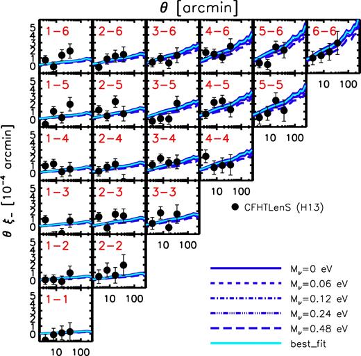
Comparison of the WMAP9-based predictions to the ξ− tomographic CFHTLenS shear measurements of Heymans et al. (2013).
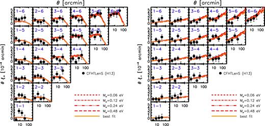
Comparison of the Planck2015/ALens-based predictions to the ξ± tomographic CFHTLenS shear measurements of Heymans et al. (2013).
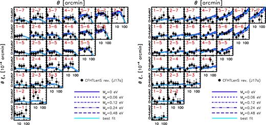
Comparison of the WMAP9-based predictions to the ξ± tomographic CFHTLenS shear measurements of Joudaki et al. (2017a).
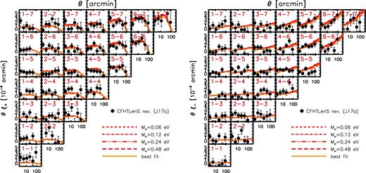
Comparison of the Planck2015/ALens-based predictions to the ξ± tomographic CFHTLenS shear measurements of Joudaki et al. (2017a).
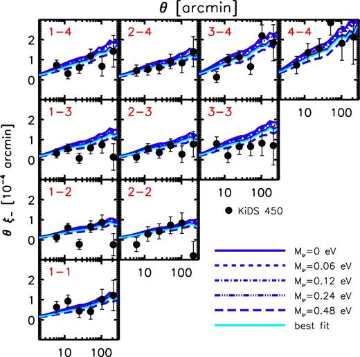
Comparison of the WMAP9-based predictions to the ξ− tomographic KiDS-450 shear measurements of Hildebrandt et al. (2017).
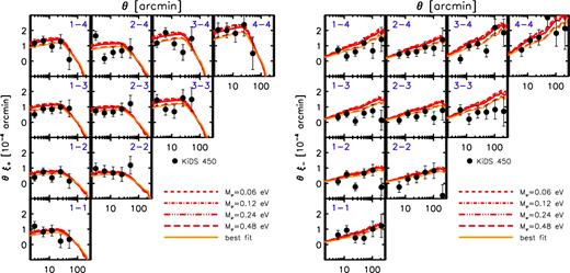
Comparison of the Planck2015/ALens-based predictions to the ξ± tomographic KiDS-450 shear measurements of Hildebrandt et al. (2017).
