


Abstract
Clusters of galaxies gravitationally lens the cosmic microwave background (CMB) radiation, resulting in a distinct imprint in the CMB on arcminute scales. Measurement of this effect offers a promising way to constrain the masses of galaxy clusters, particularly those at high redshift. We use CMB maps from the South Pole Telescope Sunyaev–Zel'dovich (SZ) survey to measure the CMB lensing signal around galaxy clusters identified in optical imaging from first year observations of the Dark Energy Survey. The cluster catalogue used in this analysis contains 3697 members with mean redshift of |$\bar{z} = 0.45$|. We detect lensing of the CMB by the galaxy clusters at 8.1σ significance. Using the measured lensing signal, we constrain the amplitude of the relation between cluster mass and optical richness to roughly |$17\,\,\rm{per\,\,cent}$| precision, finding good agreement with recent constraints obtained with galaxy lensing. The error budget is dominated by statistical noise but includes significant contributions from systematic biases due to the thermal SZ effect and cluster miscentring.
1 INTRODUCTION
Cosmic microwave background (CMB) photons passing near massive galaxy clusters are gravitationally deflected, leading to small-amplitude (typically |${\lesssim } 10 \, \mu {\rm K}$|) distortions in the observed CMB on arcminute scales. As pointed out by several authors (e.g. Seljak & Zaldarriaga 2000; Dodelson 2004; Holder & Kosowsky 2004; Vale, Amblard & White 2004; Lewis & King 2006; Hu, DeDeo & Vale 2007), these distortions can be used to measure the masses of galaxy clusters. Because gravitational lensing is sensitive to the total cluster mass, cluster masses determined from the CMB lensing signal are in principle robust to uncertainties on baryonic processes occurring inside the clusters. In contrast, cluster observables such as the thermal Sunyaev–Zel'dovich (tSZ) decrement, X-ray temperature, and cluster richness may depend on complicated baryonic physics that can introduce systematic uncertainty into the cluster mass-observable relations. Systematic uncertainty on cluster masses dominates the error budget of most recent cluster abundance constraints on cosmology (e.g. Rozo et al. 2010; Mantz et al. 2015; de Haan et al. 2016; Planck Collaboration XXIV 2016).
Cluster masses can also be inferred from gravitationally induced shearing of images of background galaxies (for a review see Hoekstra et al. 2013). However, at high redshift, measurements of cluster masses with galaxy lensing become challenging because the source galaxies become harder to detect and their shapes and redshifts become more difficult to measure (e.g. Hoekstra 2001). CMB cluster lensing, on the other hand, has the advantage that the signal to noise is roughly constant with cluster redshift (Lewis & King 2006). Furthermore, CMB cluster lensing is not sensitive to many of the sources of systematic error that affect estimates of cluster mass derived from galaxy shear, including PSF modelling errors (e.g. Jarvis et al. 2016), biases in the photometric redshift estimates of source galaxies (e.g. Melchior et al. 2017), and contamination of the shear sample with unlensed cluster galaxies (e.g. Applegate et al. 2014; Melchior et al. 2017). Consequently, even at low redshifts where CMB lensing-derived constraints on cluster masses may not be statistically competitive with galaxy lensing-derived constraints, CMB cluster lensing offers an important test of systematic errors associated with galaxy lensing.
The CMB lensing signal induced by galaxy clusters was first measured around clusters detected in the South Pole Telescope (SPT) SZ Survey by Baxter et al. (2015, hereafter B15). A similar measurement around Planck-detected clusters was performed in Planck Collaboration XXIV (2016). Both of these early measurements used the CMB cluster lensing signal to place (weak) constraints on the scaling between the lensing-derived mass and the mass inferred from measurement of the tSZ. Related work by Madhavacheril et al. (2015) used CMB lensing to constrain the mean mass of optically selected CMASS galaxies (Eisenstein et al. 2011; Dawson et al. 2013; Ahn et al. 2014) using CMB data from the Atacama Cosmology Telescope Polarimeter (ACTPol). Recently, Geach & Peacock (2017) used CMB lensing measurements derived from Planck data to constrain the masses of clusters detected in the Sloan Digital Sky Survey.
The aim of this work is to measure the CMB cluster lensing signal around galaxy clusters identified in optical imaging from year 1 (Y1) Dark Energy Survey (DES) observations and to use the measurement of CMB cluster lensing to calibrate the relation between cluster mass and optical richness. To this end, we employ the same SPT-SZ CMB temperature maps as used in B15. However, the galaxy cluster sample employed here is significantly expanded relative to that used in B15. B15 measured the CMB cluster lensing signal using 513 SZ-selected clusters; here we use 3697 clusters identified using the redMaPPer (Rykoff et al. 2014) algorithm applied to DES imaging.
This work also represents a significant departure in methodology from the B15 analysis. B15 defined a map-space likelihood for the observed CMB temperature measurements around a cluster as a function of cluster mass, and used that likelihood to constrain the stacked cluster mass of the sample. In this work, we employ the more standard quadratic estimator approach to estimate the lensing convergence, κ, in small cutouts of the CMB around the galaxy clusters. The primary advantage of the quadratic estimator approach employed here is its robustness to important sources of systematic error. With minor modification to the standard filters used to construct the quadratic estimator, we find that the estimator is fairly robust to the presence of tSZ signal around the cluster. Additionally, the quadratic estimator is less sensitive to other sources of systematic error, such as foreground lensing. Consequently, in this analysis we are able to directly use the low-noise 150 GHz CMB maps from the SPT rather than creating higher noise tSZ-free maps from multifrequency data.
We fit the stacked CMB lensing-derived κ measurements around the redMaPPer clusters to place constraints on the redMaPPer mass–richness relation. We show that two important sources of systematic error for these constraints are cluster miscentring and contamination of the lensing estimator by tSZ signal.
The structure of the paper is as follows: in Section 2 we introduce the formalism for computing κ from CMB temperature maps around clusters; Section 3 describes the SPT and DES data sets used in this work; Section 4 describes the pipeline we have developed for measuring CMB lensing around galaxy clusters; Section 5 describes the process of fitting the lensing measurements to obtain constraints on the masses of the clusters in our sample; Section 6 describes the simulations we have developed to test the analysis pipeline. Our results are described in Section 7 and discussion of these results is presented in Section 8.
Throughout this analysis we assume the best-fitting ΛCDM cosmological model from the Planck TT,TE,EE+lowP fits in Planck Collaboration XIII (2016). Cluster masses are described in terms of M200m, the mass enclosed within a sphere of radius R200m centred on the cluster. R200m is in turn the distance from the cluster centre at which the mean enclosed density is 200 times the mean density of the Universe at the redshift of the cluster.
2 A QUADRATIC ESTIMATOR FOR κ
As pointed out by Hu et al. (2007) and others, the quadratic estimator formulated by Hu & Okamoto (2002) is biased in regions of high κ. This bias can be understood as resulting from the fact that a very massive lens (such as a cluster) will magnify the CMB gradient behind it, effectively decreasing the magnitude of the estimated gradient field; the result is that the κ estimate is biased low. To remove this bias, Hu et al. (2007) showed that one could simply apply an additional low-pass filter to the maps before estimating the gradient field. This additional filter separates out the scales used to estimate the gradient from those used to measure the small-scale CMB fluctuations caused by lensing, and thereby removes the bias. The filter scale used, lG, becomes an additional parameter of the analysis, but the results are not expected to be very sensitive to variations in this scale.
In the analysis presented below, we will apply the Hu et al. (2007) quadratic estimator to estimate κ in cutouts of the SPT CMB maps around galaxy clusters. Because κ is directly related to the integrated mass along the line of sight, by fitting a model to the recovered κ we can extract constraints on the masses of the clusters in our sample.
3 DATA
3.1 CMB maps from SPT
The SPT is a 10-metre millimetre/submillimetre telescope operating at the geographical South Pole (Carlstrom et al. 2011). The CMB maps used in this analysis are from the 2500 deg2 SPT-SZ survey, which mapped the sky in three frequency bands centred at 95, 150, and 220 GHz over an observation period from 2008 to 2011 (Story et al. 2013). We use only the SPT 150 GHz maps in this analysis as these have the lowest noise.
SPT observations are divided into patches of the sky (fields) that each have an area ≳100 deg2. For most fields, SPT scans the sky in strips of constant elevation, first moving left, then right, followed by a step in elevation. For one field (ra21hdec-50), a modified scanning strategy was used for some observations, but we use only the azimuthal scan data from that field in this analysis. The time ordered data from these scans is filtered to prevent aliasing of high-frequency noise and to remove atmospheric and instrumental noise. The time ordered data is processed into maps with 0.5 arcmin resolution using the Lambert equal-area azimuthal projection. The maps used here are identical to those used in the George et al. (2015, hereafter G15) analysis, and we refer readers to that work for more details of the map making process.
The signal on the sky observed with the SPT is modified by a response function consisting of a beam function and a transfer function. The beam function describes the smearing of sky sources as a result of the finite aperture of the SPT primary mirror. The transfer function accounts for time-domain filtering applied to the SPT signal. The total SPT response function to a mode |$\boldsymbol {l}$| on the sky can be modelled as the product |$B(l)T(\boldsymbol {l})$|, where B(l) and |$T(\boldsymbol {l})$| are the beam and transfer functions, respectively, and B(l) only depends on |$l = |\boldsymbol {l}|$| since the beam is close to rotationally invariant.
The amount of time spent observing each field in the SPT-SZ survey is not constant, and the effective depth across a field varies slightly as a result of scanning strategy. To characterize the varying depth levels between fields and within a field, we define the weight, ωi, at map pixel i. The weight is roughly proportional to the inverse variance of the map noise at that pixel. We will use maps of the weight across the sky to calculate the appropriate noise power spectrum for each cluster cutout.
Before computing κ from the CMB maps, point sources detected in the maps at 5σ are masked and inpainted with Gaussian noise that matches the noise level of the SPT maps. The point source catalogue used for this purpose is the same as used in George et al. (2015) for masking.
3.2 redMaPPer cluster catalogue from DES
DES is a five-year optical imaging survey of 5000 deg2 of the southern sky using the Dark Energy Camera on the Blanco Telescope (Flaugher et al. 2015). In this analysis, we make use of first year (Y1) DES data, which covers roughly 1800 deg2 of sky (Diehl et al. 2014; Drlica-Wagner et al. 2017). The total area of overlap between Y1 observations and the SPT-SZ survey is roughly 1500 deg2.
Galaxy clusters were identified in the Y1 data using the redMaPPer algorithm (Rykoff et al. 2014). The application of redMaPPer to early DES Science Verification (SV) data is described in Rykoff et al. (2016). The application of redMaPPer to Y1 data will be described in more detail in an upcoming publication (McClintock et al. in preparation). redMaPPer identifies cluster candidates as overdensities of red-sequence galaxies on the sky. For each cluster candidate, redMaPPer determines a list of possible cluster member galaxies and their corresponding membership probabilities. The redMaPPer estimate of the cluster richness, λ, is defined as the sum over these membership probabilities for each cluster. redMaPPer also computes centring probabilities, Pcen, which characterize the probability that a member galaxy is at the centre of the cluster. We treat the galaxy with the highest Pcen as the cluster centre in this analysis, but also consider the effects of various degrees of miscentring. We will also use the redMaPPer estimates of the cluster redshifts in this analysis; these are expected to be accurate to roughly σz ∼ 0.01(1 + z).
We consider only the volume-limited redMaPPer DES Y1 catalogue, restricted to clusters with richness λ > 20, resulting in a total of 7066 clusters. We further impose the requirements that the minimum SPT-defined weight in a ∼2° × 2° cutout around the cluster (see Section 4 for a more detailed description of the cutouts) is greater than zero and is at least 80 per cent of the weight at the cluster location. These restrictions ensure that we do not include clusters outside of the SPT fields or clusters for which the weight is varying significantly across the cutout (as may occur near the field boundaries). After imposing this restriction, the cluster catalogue is reduced to 4552 clusters. Finally, as will be described in more detail in Section 7.3.1, we find that the presence of tSZ signal around high-mass clusters can bias the κ reconstruction. Because the amplitude of the tSZ signal scales as M5/3, by restricting our analysis to lower mass clusters we find that we can reduce the tSZ bias to acceptable levels while preserving much of the lensing signal. To this end, we employ a somewhat conservative richness cut, restricting our analysis to λ < 40. This richness threshold corresponds to a mass of about 3.2 × 10¹⁴ M⊙ assuming the mass–richness relation of Melchior et al. (2017, hereafter M17). We discuss the motivation for the richness cut and tests of potential tSZ biases in more detail in Section 7.3. Imposing the richness cut yields a final catalogue of 3697 clusters ranging in redshift from roughly z ∼ 0.1 to 0.7, with mean redshift |$\bar{z} = 0.45$|.
4 MEASUREMENT OF κ
For each DES-identified cluster, we estimate κ using cluster-centred cutouts from the SPT 150 GHz temperature maps presented in G15. The CMB temperature maps are pixelized at 0.5 arcmin resolution and the cutouts are 256 pixels on a side.
We rotate each cutout so that it is aligned along lines of constant azimuth and elevation (see e.g. Schaffer et al. 2011 for description of the rotation angles corresponding to the Lambert equal-area azimuthal projection). Aligning the cutouts with altitude and azimuth ensures that the transfer function is the same for every cutout, significantly simplifying the subsequent analysis. Rotation is performed using third-order spline interpolation. The rotated cutouts are then apodized using a Tukey window with α = 0.1. Our analysis of simulated data in Section 6 confirms that this choice of apodization is reasonable.
4.1 Noise and foregrounds
Estimating κ near each cluster requires an estimate of the noise power spectrum in each CMB temperature cutout. We consider as noise any contribution to the cutouts that is not CMB and that is not expected to be correlated with the positions of the galaxy clusters. Non-CMB signal that is correlated with the clusters – such as the cluster tSZ signal – is treated as a source of systematic error and is discussed in Section 7.3. Each cutout receives contributions from astronomical, atmospheric, and instrumental noise sources. We will take a model-based approach to estimating the contributions from astronomical noise sources; we estimate the contribution from atmospheric and instrumental noise directly from the data.
We first consider the contribution to the cutouts from astronomical noise sources; such noise is constant over the time-scale of the observations. In addition to the CMB, the sky signal at 150 GHz receives significant contributions from several sources, including galaxies that are bright at microwave frequencies and unresolved tSZ signal. The relative contributions of these various sources is l-dependent: at low multipoles (ℓ ≲ 3000), the CMB dominates while at higher multipoles (ℓ ≳ 3000), foreground emission becomes dominant. In general, the astrophysical foreground sources can be approximated as Gaussian random noise. Although foreground emission from extragalactic sources such as dusty galaxies and the tSZ are known to be non-Gaussian at some level (e.g. Crawford et al. 2014), the Gaussian approximation should be sufficient for the noise levels considered here (van Engelen et al. 2014). The SPT CMB maps also receive some contribution from galactic foregrounds, such as dust. However, this foreground contribution is expected to be significantly below the contributions from the other foregrounds mentioned above (e.g. Keisler et al. 2011).
Once bright point sources have been removed, the dominant foreground contribution to the sky at 150 GHz comes from dusty, star-forming galaxies (DSFGs). The power spectrum of DSFG emission can be divided into two components: one arising from sources on the sky that are unclustered, and another arising from sources that are clustered on the sky. The unclustered component has an angular power spectrum given by Cl = C0, where C0 is a constant. Expressed in terms of Dl = l(l + 1)Cl/(2π), the analysis of G15 found |$D_{3000} = 9.16 \pm 0.36 \, \mu {\rm K}^2$| for the unclustered component. The clustered DSFG component, on the other hand, can be modelled with Dl ∝ l0.8 for l > 1500. The G15 analysis found |$D_{3000} = 3.46\pm 0.54 \, \mu {\rm K}^2$| for this component. For l < 1500, the contribution of the clustered DSFG foreground can be ignored.
Two other significant foreground contributors at 150 GHz are radio galaxy emission below the detection threshold of SPT maps and the tSZ signal from undetected galaxy groups or clusters. Following G15, we model the signal from radio galaxies below the SPT detection threshold as an unclustered component with |$D_{3000} = 1.28\,\mu {\rm K}^2$|. To model the tSZ signal from sources below the detection threshold we use the templates from Shaw et al. (2010), normalized using the constraint from G15. G15 constrained the amplitude of the tSZ power spectrum after masking sources above the detection threshold to be |$D_{3000} = 2.33^{+0.8}_{-1.4}\,\mu {\rm K}^2$|, and we use this value here.
For our fiducial analysis we make the simplifying approximation that all emission from astrophysical foregrounds is unlensed by the galaxy clusters. In reality, this approximation is not very good. The cosmic infrared background (CIB), for instance, is expected to receive significant contribution from redshifts 1 < z < 3 (e.g. Béthermin et al. 2013). Because the clusters used in this analysis have |$\bar{z} = 0.45$|, a significant portion of the CIB may be lensed by the clusters. However, the precise redshift distribution of the DSFGs and other foreground sources is not known, making modelling of foreground lensing difficult. While treating the foregrounds as unlensed is incorrect at some level, we will show in Section 7.3.2 that this simplifying assumption has little effect on our results.
Unlike astrophysical foregrounds, the contribution from atmospheric and instrumental noise sources is not constant over the SPT observation time, allowing us to estimate the contributions to the noise power spectrum from these sources by differencing maps constructed from observations taken at different times. As described in Section 3.1, SPT fields are observed by scanning the telescope left and right across the full field at a series of discrete elevations. We can form a signal-free map as the combination |$\boldsymbol {m}^{\rm diff} = (\boldsymbol {m}_{\rm L} - \boldsymbol {m}_{\rm R})/2$|, where |$\boldsymbol {m}_{\rm L}$| and |$\boldsymbol {m}_{\rm R}$| are the maps formed from left and right-going scans, respectively. Because atmospheric and instrumental noise vary on time-scales that are much shorter than the time difference between the |$\boldsymbol {m}_{\rm L}$| and |$\boldsymbol {m}_{\rm R}$| observations, |$\boldsymbol {m}^{\rm diff}$| should provide a realization of the instrumental and atmospheric noise.
The SPT-SZ survey spent different amounts of time observing each field, resulting in field-to-field variations in the effective noise levels of the resultant CMB maps. Additional variation in the noise levels between and within fields occurs as a result of sky projection. To account for field-to-field variation in the noise level, each cluster is analysed using the difference maps for the field in which it was observed. To account for variation in the noise level across the field, we use the SPT weight maps, |$\boldsymbol {\omega }$|.
We first construct a scaled difference map that has effectively uniform weight by multiplying the map by |$\sqrt{\boldsymbol {\omega }/\langle \omega \rangle }$|, where 〈ω〉 is the mean weight across the inner [0.3, 0.7] of the map. We then compute the instrumental and atmospheric noise power spectrum at the mean weight using this scaled difference map. To determine the estimate of the instrumental and atmospheric noise power spectrum for the ith cutout we then rescale the noise power spectrum estimate for the scaled difference map by 〈ω〉/ωi, where ωi is the mean weight across the ith cutout.
4.2 Stacked, filtered κ estimate
Given the beam and transfer function deconvolved cutouts and the estimate of the noise power spectrum in the cutout, we compute κ across the cutouts as described in Section 2. When generating the κ estimate for each cutout we use a gradient filter scale of lG = 1500. In principle, higher signal to noise could be achieved by setting lG = 2000 as originally suggested by Hu et al. (2007). However, we have found in tests on simulated data (see Section 7.3.1) that the tSZ signal from massive clusters can lead to a significant bias in the recovered mass when using lG = 2000. By using the lower value of lG = 1500, we find that this bias can be significantly reduced without significantly degrading the signal to noise. The low-pass filter removes some of the highly localized tSZ signal while preserving most of the information about the large-scale gradient in the CMB near the cluster.
By deconvolving the beam function from the cutouts, we increase the effective noise of small-scale modes that are heavily filtered by the beam [e.g. equation (14)]. Such small-scale noise is problematic for our analysis since we attempt to fit the κ profiles of the clusters in real space. In real space the filtered scales are not cleanly separated from the unfiltered scales, and the resultant small-scale noise introduces numerical problems. To reduce the effects of such noise, we filter the κ cutouts with a low-pass filter to remove modes with |$l < \sqrt{8 \ln 2}/\theta _{{\rm FWHM}}$|, where θFWHM = 1.3 arcmin is chosen to roughly match the beam size of the SPT.
Because the estimate of κ at the cluster location depends on the gradient of the CMB temperature field, there is useful information for constraining κ in the temperature maps at scales well beyond the halo virial radius. However, once the estimate of κ has been computed, areas of the κ cutout that are well beyond the virial radius of the cluster do not contain significant information about the halo density profile.1 We can therefore speed up our analysis pipeline with little reduction in signal to noise by restricting our analysis to the inner parts of the κ cutouts. To this end, we restrict our fitting to the inner 10 arcmin × 10 arcmin region at the centre of the full κ cutouts. The size of this reduced cutout can be compared to the halo virial radius of a M = 5 × 10¹⁴ M⊙ halo at the mean redshift of the cluster sample (|$\bar{z} = 0.45$|), which is ∼5 arcmin. As noted previously, the richness limit imposed in this analysis corresponds to roughly 3.25 × 10¹⁴ M⊙, so restricting the analysis to the inner 10 arcmin captures the region within the virial radius for the majority (if not all) of the clusters in our sample. To reiterate: we use large 128 arcmin × 128 arcmin cutouts of the CMB temperature maps to estimate κ, but we only use the inner 10 arcmin × 10 arcmin of the resulting κ map for cluster mass estimation.
Even if the true κ in the cutout is zero, the application of the quadratic estimator to the cutout is still expected to return a non-zero estimate of κ because of the apodization window that is applied. To estimate the true κ, then, we must subtract an estimate of the mean κ in the absence of any CMB lensing, i.e. the mean field. We form an estimate of the mean field for each observation field by performing the κ estimation process around random locations within the field. The number of random points is approximately 40 times the number of clusters in each field, and we confirm that the scatter in the mean field estimate for each field is negligible compared to the noise in the κ estimate around the clusters.
Because the SPT transfer function is anisotropic, the κ cutouts necessarily have anisotropic noise. We therefore fit the stacked 2D |$\boldsymbol {\kappa }_s$| cutout in our analysis rather than the azimuthally averaged profile of this cutout, as will be described in more detail below. To estimate the covariance of |$\boldsymbol {\kappa }_s$| we use jackknifing.
5 FITTING THE κ MEASUREMENTS
5.1 Model
We fit the 2D stacked |$\boldsymbol {\kappa }_s$| measurement to constrain the relation between M200m and λ for the clusters in our sample. Each cluster is modelled as the sum of a ‘1-halo’ term resulting from the mass of the cluster itself, and a ‘2-halo’ term resulting from correlated structure along the line of sight.
By comparing redMaPPer centres identified in DES SV data measurements in X-ray and SZ, Rykoff et al. (2016) constrained the fraction of miscentred clusters in DES SV data to be fmis = 0.22 ± 0.11. Rykoff et al. (2016) modelled the assumed cluster centre as being a draw from a two-dimensional Gaussian with variance |$\sigma _R^2$| centred on the true cluster centre. In this model, Rmis follows a Rayleigh distribution which peaks at σR. Rykoff et al. (2016) further assumed that σR was proportional to the redMaPPer defined cluster radius, Rλ = (λ/100)0.2 h−1 Mpc, and constrained σR = cmisRλ with ln cmis = −1.13 ± 0.22.
5.2 Likelihood analysis
Constraints on the mass–richness parameters. Top-hat distributions are indicated by brackets, while Gaussian distributions are written in the form a ± b.
| Parameter | Prior | Posterior |
|---|---|---|
| A/M⊙ | [1012, 1016] | (2.14 ± 0.35) × 1014 M⊙ |
| α | 1.23 ± 0.30 | 1.25 ± 0.30 |
| β | 0.18 | – |
| Parameter | Prior | Posterior |
|---|---|---|
| A/M⊙ | [1012, 1016] | (2.14 ± 0.35) × 1014 M⊙ |
| α | 1.23 ± 0.30 | 1.25 ± 0.30 |
| β | 0.18 | – |
Equation (25) ignores several potential sources of uncertainty in the stacked model, |$\boldsymbol {\kappa }_s^m$|. First, we have ignored scatter in the mass–richness relation. This scatter is expected to be described by a lognormal probability distribution function, with scatter at fixed λ given by σln M|λ ∼ 0.25 (e.g. Rozo & Rykoff 2014). At low richness, one expects increased scatter due to the Poisson uncertainty in the number of galaxies. However, even accounting for the additional Poisson scatter (following the prescription described in S17) we find that the uncertainty on |$\boldsymbol {\kappa }_s^m$| is much less than the uncertainty on the measurement vector, |$\boldsymbol {\kappa }_s$|. Consequently, without introducing any measurable bias in our results, we can ignore scatter in the mass–richness relation.
Additionally, equation (25) ignores uncertainty in the redshift and richness estimates for the clusters. The typical redshift uncertainty for DES redMaPPer clusters is σz/(1 + z) ≲ 0.01 (Rykoff et al. 2016). For this level of redshift uncertainty, the resultant uncertainty in |$\boldsymbol {\kappa }_s^m$| is much less than the uncertainty in the κ measurements, so it is safe to ignore redshift uncertainty in this analysis. A similar argument holds for the uncertainty on the richness estimates.
Finally, note that equation (25) ignores correlated scatter between the richness and lensing mass. Such correlated scatter is expected because clusters that are elongated along the line of sight will have enhanced richness and lensing masses. However, the impact of such correlated scatter is expected to be at the few percent level (Melchior et al. 2017), well below the statistical uncertainties obtained here. For simplicity we therefore ignore this effect.
6 PIPELINE VALIDATION
We use simulated SPT observations to test the κ estimation pipeline. We generate simulated SPT maps by adding together Gaussian realizations of the CMB, foreground and noise. The CMB realizations are generated from a power spectrum computed at our fiducial cosmological model using CAMB2 (Lewis, Challinor & Lasenby 2000).
We lens the simulated CMB maps with mock clusters described by the NFW profile of equation (16). To perform the lensing operation, we compute the deflection angles for these clusters using the formulae of Bartelmann (1996). The unlensed CMB is then remapped to the lensed CMB with cubic spline interpolation. The main purpose of the simulations is to confirm that our lensing pipeline recovers an unbiased estimate of κ to within our noise levels. We therefore use clusters of fixed mass and redshift when generating the simulations. We use 100 mock galaxy clusters that are roughly equally spaced across the field. Each simulated cluster has M = 2.5 × 10¹⁴ M⊙, z = 0.4 and c = 4.8. This mass is somewhat higher than the mean mass predicted for the redMaPPer sample based on the mass–richness relation of M17, which is M ∼ 2.05 × 10¹⁴ M⊙.
Foreground emission is generated as Gaussian random realizations of the foreground models described in Section 4.1 and added to the lensed CMB maps. We assume that foreground emission is unlensed by the galaxy clusters when generating the simulated maps because this matches the assumption of our fiducial analysis; we consider the effects of this assumption on the analysis of the real data in Section 7.3.2. Note that for the purposes of pipeline validation, we do not include tSZ signal in the simulated data; we estimate the effects of tSZ contamination in Section 7.3.1.
The simulated sky maps are then convolved with the beam and field-dependent transfer functions from G15. Finally, field-dependent noise realizations are added to the simulated maps. To generate the field-dependent noise realizations, we generate Gaussian random realizations of the estimated noise power spectrum from the weight-scaled difference maps described in Section 4.1. The noise realizations are then scaled by the inverse square root of the weight to account for weight variations across the field.
To build statistics, we generate 200 simulated skies using the methods described above. Each simulated sky map is lensed with 100 clusters, bringing the total number of simulated clusters to 20 000. Each simulated sky has a different random realization of the CMB, foregrounds and noise. The simulated skies are passed through the same pipeline that is applied to the data to extract κ cutouts around each of the simulated clusters. The κ cutouts are then fit to determine constraints on the cluster mass, M200m.
Fig. 1 shows the true, azimuthally averaged κ profile (red) in the simulations compared to the κ profile recovered using our analysis pipeline (points with error bars). The oscillatory behaviour of κ comes from application of the filter described in Section 4.2 to the κ cutouts. The pipeline recovers an unbiased estimate of κ to within the uncertainties of the mock data. Note that we have used roughly five times as many simulated clusters as real clusters for this test to increase our sensitivity to any possible biases in the κ estimation.
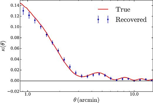
Azimuthally averaged κ profile recovered from analysis of simulated data. Red solid curve shows the true κ profile around mock clusters with M = 2.5 × 10¹⁴ M⊙ after the application of the filtering described in Section 4.2. Blue data points with errorbars show recovered κ in the presence of realistic noise, foreground emission, beam, and transfer function using 20 000 clusters. The measurement pipeline recovers an unbiased estimate of the true κ profile to within the uncertainties.
7 RESULTS
7.1 κ measurements around redMaPPer clusters
Fig. 2 shows the weighted average of the κ cutouts around redMaPPer clusters, restricted to the region used in fitting. Pixels in the κ cutouts are 0.5 arcmin on a side and the fitted region is 20 pixels by 20 pixels. Because the centres of the redMaPPer clusters do not lie at exactly the same position in each map pixel, Fig. 2 incorporates some smearing due to pixelization effects. However, when fitting for the parameters of the mass–richness relation we use the full coordinate information for each pixel relative to the true cluster centres on a cluster-by-cluster basis.3
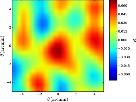
The stacked, weighted 2D κ profile recovered from the analysis of CMB temperature data around 3697 redMaPPer clusters. Each pixel in the cutout is 0.5 arcmin on a side.
Fig. 3 shows the azimuthally averaged one-dimensional κ profile extracted from the analysis of redMaPPer clusters. To determine the error bars shown in this plot we use a jackknife resampling approach, where the jackknife subsamples are determined by dividing survey area into 100 regions of approximately equal area. The data exhibit a strong preference for increasing κ towards the centre of the cluster, as expected. We note, though, that adjacent measurements in Fig. 3 are highly correlated. While we show the 1D κ profile here for the purposes of visualization, our analysis to extract mass constraints on the clusters uses the full 2D κ information, rather than the 1D azimuthally averaged profile.
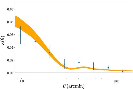
The azimuthally averaged κ profile recovered from measurement of CMB lensing around 3697 redMaPPer clusters detected in DES Y1 data (blue points with errorbars). The errorbars shown are the diagonal elements of the full covariance determined from a jackknife resampling of the cluster sample; there is significant covariance between adjacent data points. The orange region indicates the allowed range of model predictions (68 per cent confidence region) given the results of the fit for parameters of the cluster mass–richness relation.
7.2 Fit results
The 2D and marginalized posteriors on the mass–richness parameters A and α recovered from our analysis are shown in Fig. 4; numerical results are given in Table 1. We find A/M⊙ = (2.14 ± 0.35) × 1014, a roughly 17 per cent constraint on the amplitude of the mass–richness relation. The posterior on α is entirely dominated by the prior (shown as the blue curve). This is not surprising given the fairly low signal to noise of our measurement and the fact that the richness range of the sample is restricted to 20 < λ < 40. There appears to be minimal degeneracy between A and α over the range of α allowed by the constraints of M17 and S17. If we fix α to the best-fitting value from M17, we find that the best-fitting A changes by only 1 per cent and the error on A decreases by only 2 per cent. Because our prior on α is quite wide, our results are therefore very robust to assumptions about α.
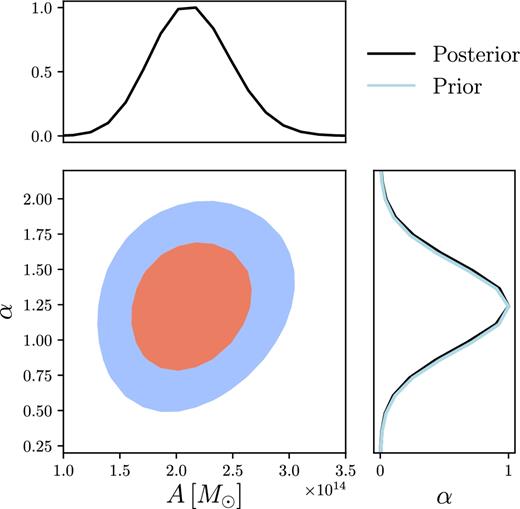
Constraints on the amplitude, A, and richness scaling, α, of the redMaPPer mass–richness relation obtained from fits to CMB lensing measurements. Contours represent 1σ and 2σ levels. The blue curve in the panel at right shows the prior on α, which dominates our constraint. Numerical results are summarized in Table 1.
We find |$\Delta \ln \mathcal {L} = 33.3$| between the peak of the likelihood and A = 0; a likelihood ratio test therefore allows us to reject the null hypothesis that A = 0 at 8.1σ significance. The significance of this detection can be compared to the 3.1σ detection obtained in B15 from 513 clusters. Those clusters were approximately twice as massive as the ones considered here, so we would expect that despite the increase in sample size our current measurement would yield a ∼4.0σ detection. The higher detection significance reported here is the result of the switch from the tSZ-free maps used in B15 to the lower noise 150 GHz SPT maps that we are able to use with the quadratic estimator in the current analysis.
7.3 Systematic errors
7.3.1 tSZ
The tSZ effect is caused by inverse Compton scattering of CMB photons with energetic electrons. The effect is especially pronounced in the direction of massive galaxy clusters, as these objects are reservoirs of hot gas. At 150 GHz – the frequency of observation for the CMB maps used in this analysis – the tSZ effect leads to a decrement in the observed CMB temperature near the cluster (for a review see Birkinshaw 1999). We do not attempt to model the tSZ in this analysis; consequently, its presence acts as a potential source of bias to our measurement of κ. Somewhat worryingly, the magnitude of the tSZ decrement for a massive cluster can be |${\sim } 100\, \mu {\rm K}$|, significantly larger than the magnitude of the CMB cluster lensing-induced distortion, which has amplitudes |${\lesssim } 10\, \mu {\rm K}$|. However, the situation is not so bad as it might first appear: unlike the CMB cluster lensing signal, the tSZ effect is not correlated with the CMB gradient behind the cluster. Because the quadratic estimator used to measure the lensing distortion is effectively picking out correlations between small-scale CMB distortions and the larger scale gradient field, it is expected to be fairly robust to tSZ contamination. Furthermore, the low-pass filtering imposed on the CMB maps to estimate the gradient field (Section 2) effectively filters out the small-scale tSZ decrements, reducing their contamination of the κ estimator. Finally, as noted in Section 3.2, we restrict our analysis to clusters with λ < 40 to reduce the amplitude of tSZ contamination.
To constrain the level of systematic error introduced to our κ estimates by the tSZ we rely on simulations. We introduce mock tSZ signals into the simulations described in Section 6 and re-analyse these simulations to determine how much the κ estimation is biased. The mock tSZ signals used for this purpose are taken from the hydrodynamical simulations of Le Brun et al. (2014). These simulations represent an extension of the OverWhelmingly Large Simulations project (Schaye et al. 2010), and are designed with applications to cluster cosmology in mind. To this end, the simulations are large volume (400 h−1 Mpc on a side) and include computation of maps of the Compton y parameter. We use their AGN 8.0 model in this analysis.
To introduce tSZ into our simulations, we extract tSZ cutouts measuring 256 arcmin on a side from the Le Brun et al. (2014) Compton y maps at the locations of massive haloes. We restrict the cutouts to those haloes with 1.75 × 10¹⁴ M⊙ < M < 3.25 × 10¹⁴ M⊙ and 0.24 < z < 0.56, as these should be well matched to the real clusters.4 A cluster with mass M200m ∼ 3.25 × 10¹⁴ M⊙ corresponds roughly to a richness of λ ∼ 40 assuming the mass–richness relation of M17. While some clusters with λ ∼ 40 in our sample may have masses larger than 3.25 × 10¹⁴ M⊙ owing to scatter in the mass–richness relation, we expect the constraint to be dominated by clusters below this mass. Comptonization maps are converted to temperature units assuming an observation frequency of 150 GHz. This process yields 135 simulated tSZ cutouts.
The simulated tSZ cutouts are added to simulated temperature maps at the locations of the mock clusters. We perform the κ estimation process on 2700 mock clusters with added mock tSZ signal. For each cluster, the tSZ signal is rotated by a random angle. With the mock tSZ profiles added to the simulations, the application of the beam, transfer function and noise then proceeds as before and the cutouts are processed through the κ estimation pipeline. The results of this analysis are then compared to a set of simulations that are identical in every way (i.e. the same realizations of CMB, noise, and foregrounds) except they do not have the added tSZ component.
Analysing the simulated cutouts with the mock tSZ signal reveals that the recovered mass in the presence of tSZ is biased low relative to the mass in the absence of tSZ by a few percent. This level of bias is significantly smaller than the statistical errors associated with our κ estimates.
There is some systematic uncertainty in the simulated tSZ profiles resulting from differences between the Le Brun et al. (2014) simulations and real galaxy clusters. Le Brun et al. (2014) showed that their simulations were able to accurately reproduce the relation between integrated Compton parameter and mass for a set of nearby galaxy clusters observed by Planck Collaboration XI (2011) and Planck Collaboration IV (2013). However, there is significant scatter between the different ‘sub-grid’ physics models considered by Le Brun et al. (2014). To account for this, we repeat the process of introducing the simulated tSZ profiles into the mock data after increasing the amplitude of the simulated tSZ profiles by 30 per cent. With this increased tSZ amplitude, we find that the bias in the recovered mass estimate increases to roughly 11 per cent. Again, this level of bias is smaller than our statistical error bar, but is certainly non-negligible. We emphasize that this bias is one-sided: it acts to reduce the inferred amplitude of the recovered κ estimate.
We have also repeated the above analysis using a more aggressive gradient filter scale of lG = 2000. This choice yields a higher signal to noise reconstruction of the cluster profile in the absence of tSZ. However, in the presence of tSZ (with amplitude fixed to that of the Le Brun et al. 2014 simulations), choosing lG = 2000 results in recovered mass estimates that are biased low by as much as 30 per cent. Our fiducial choice of lG therefore has the effect of significantly reducing the bias due to tSZ at the cost of increasing our error bars somewhat.
As a further test of tSZ contamination, we also consider the effect of varying the maximum richness threshold imposed in our analysis of the redMaPPer clusters. Because the amplitude of the tSZ signal for a cluster of mass M scales roughly as M5/3 while the lensing signal is roughly proportional to M, we expect high-richness clusters to be more impacted by tSZ bias. Indeed, we find that very high-richness clusters (λ > 100) tend to exhibit a preference for low masses. One cluster with richness λ ∼ 180 in particular exhibits a fairly significant preference for negative mass. As a result, if we include all the clusters in the analysis, the preference for A > 0 actually decreases slightly. However, when varying the richness threshold between 40 < λ ≲ 50, the preference for A > 0 tends to increase with increasing richness threshold. This suggests that tSZ contamination is fairly minimal for clusters in this richness range.
Another way to constrain the presence of tSZ bias in our analysis is to look at the posterior on α. Because high-richness clusters are expected to have their κ estimates biased low by the presence of tSZ, if such bias were significant in our measurement, we would expect the recovered posterior on α to prefer low values. Fig. 4 shows both the prior and posterior on α. The posterior on α is entirely consistent with the prior, suggesting that α is not being driven low by tSZ bias.
In addition to the tSZ effect, galaxy clusters are also expected to distort the CMB via the kinematic SZ effect (kSZ), caused by inverse Compton scattering of CMB photons with electrons that have large bulk velocities relative to the CMB frame. The kSZ is expected to be significantly smaller than the tSZ in most cases, and like the tSZ it is uncorrelated with the CMB gradient behind the cluster. Furthermore, since the sign of the kSZ signal depends on the direction of the cluster peculiar velocity relative to the line-of-sight direction, its effects should be suppressed in an average across many clusters. Consequently, the impact of kSZ on our analysis is expected to be negligible.
7.3.2 Foreground lensing
Our fiducial analysis assumes that all foreground emission is unlensed by the galaxy clusters. However, as described in Section 4.1, some foreground emission may be sourced from behind the cluster and will therefore be gravitationally lensed by the cluster. To determine the bias introduced into our analysis by the assumption of unlensed foreground, we repeat the analysis of the data assuming instead that all foreground emission originates from the surface of last scattering, and is therefore maximally lensed. In that case, the power spectrum of the foreground emission can be simply added to the CMB power spectrum when computing the quadratic estimator. These two extreme assumptions – no foreground lensing or maximal foreground lensing – bracket the possible levels of foreground lensing, and the difference between the two resultant κ estimates provides an (over)estimate of the systematic error introduced into our analysis by our foreground lensing assumption.
When we repeat the analysis of the data with the alternate foreground lensing assumption, we find that the change to the resultant mass constraints is less than |$1\,\,\rm{per\,\,cent}$|, well below our statistical uncertainty.
7.3.3 Miscentring
Our analysis assumes the best-fitting values for the miscentring parameters from Rykoff et al. (2016): fmis = 0.22 and ln cmis = −1.13. However, the Rykoff et al. (2016) constraints on the miscentring parameters carry non-negligible uncertainty. To quantify the impact of this uncertainty on our mass–richness constraints, we repeat our analysis with the miscentring parameters increased an amount equal to the 1σ uncertainties from Rykoff et al. (2016): σ(fmis) = 0.11 and σ(ln cmis) = 0.22.
We find that perturbing fmis and ln cmis by these uncertainties results in changes to A of 3 per cent and 4 per cent, respectively. Adding these uncertainties in quadrature, we therefore introduce a 5 per cent systematic uncertainty to our mass constraints to account for uncertainty on redMaPPer miscentring. This level of uncertainty is roughly |$29\,\,\rm{per\,\,cent}$| of our statistical uncertainty.
It may be surprising that uncertainty on the miscentring parameters introduces such a large systematic error on our mass constraints. Using cluster-galaxy lensing and a similar miscentring model, M17 found that miscentring introduced less than a 1 per cent error on the normalization of the mass–richness relation. This difference in amplitude can be understood as resulting from the different angular scales that contribute to the two constraints. As seen in Fig. 3, the inner most data points exclude M = 0 with high significance, suggesting that most of our constraining power is coming from small angular scales where miscentring can have a large impact. The constraint from M17, on the other hand, receives a large contribution from larger scales at which miscentring is unimportant. Indeed, fig. 11 of M17 shows that most of their signal comes from R > 1 Mpc, where the effects of miscentring are essentially negligible.
8 DISCUSSION
8.1 Cluster mass constraint from CMB cluster lensing
We have presented a 8.1σ detection of CMB cluster lensing around redMaPPer clusters. Our analysis relied on CMB temperature maps from the SPT-SZ survey and a sample of optically selected galaxy clusters identified in Y1 DES imaging. By fitting the CMB-κ measurements around the redMaPPer clusters, we constrained the amplitude of the mass–richness relation to roughly 17 per cent statistical precision.
Our systematics analysis suggests that the dominant systematics affecting our constraints on the redMaPPer mass–richness relation are cluster miscentring and the presence of tSZ. Cluster miscentring contributes a roughly 5 per cent systematic error to our mass constraints. Our analysis attempts to minimize bias due to the tSZ by restricting the cluster sample to λ < 40 and applying a conservative filter when estimating the CMB temperature gradient field. To estimate residual bias due to the presence of tSZ we analyse simulated data with tSZ profiles taken from the AGN 8.0 simulations of Le Brun et al. (2014) and also employ a data-only consistency test. Both of these tests suggest that there is negligible bias in our analysis due to the tSZ. However, after adjusting the simulations to (conservatively) account for uncertainty in the mock tSZ profiles, we find that the tSZ-caused bias increases to 11 per cent. Note that this bias acts to reduce the inferred amplitude of the mass–richness relation, and so should not be thought of as a two-sided uncertainty.
8.2 Comparison to other redMaPPer lensing measurements
The results presented in this work represent the first weak lensing mass calibration of the DES Y1 redMaPPer clusters, and therefore a direct comparison of these results to other weak lensing measurements with the same cluster sample is not yet possible. However, given that the redMaPPer mass–richness relation is expected to be survey-independent to a good approximation, it is possible to compare our results to other recent redMaPPer weak lensing mass constraints.
Fig. 5 compares the constraint obtained here on the cluster mass–richness relation to other constraints obtained from cluster-galaxy lensing. We evaluate all of the various mass–richness relations at z = 0.5, the pivot redshift of this analysis and that of M17. The most direct comparison to this work is with the weak lensing mass calibration of DES SV clusters by M17, since that work used the same telescope and similar modelling assumptions. Our constraint on the redMaPPer mass–richness relation is in good agreement with the constraint from M17 over the richness range considered in this work. We prefer a slightly lower normalization of the mass–richness relation, but this difference is not statistically significant. Note that our analysis uses ∼3700 clusters, while the M17 analysis used only ∼1600 clusters. Our constraint on the mass–richness relation is also in good agreement with recent constraints on the mass–richness relation of redMaPPer clusters in SDSS by S17, shown as the yellow band in Fig. 5. To translate the S17 constraint from the mean redshift of the SDSS sample to z = 0.5, we have assumed the redshift scaling and uncertainty from the M17 analysis, i.e. β = 0.18 ± 0.75. Were we to instead evaluate the S17 mass–richness relation at the mean redshift of the clusters in that work, the uncertainty on the mass–richness relation would be significantly reduced. Finally, we note that unlike the analyses of M17 and S17, we have imposed an informative prior on α in our analysis (see Table 1). However, as shown in Fig. 4, α is not significantly degenerate with A, given the prior used on α.
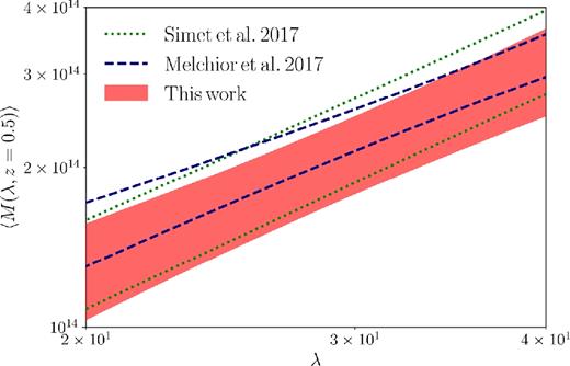
Comparison of constraints obtained on the redMaPPer mass–richness relation from CMB cluster lensing (this work) and cluster-galaxy lensing (Melchior et al. 2017; Simet et al. 2017). The solid band and lines illustrate the 1σ ranges allowed by the different constraints. Note that unlike the Melchior et al. (2017) and Simet et al. (2017) analyses, this work imposes an informative prior on the slope of the mass–richness relation.
8.3 Future prospects
As noted in Section 1, CMB cluster lensing can be used to provide constraints on systematic errors associated with other weak lensing cluster mass constraints. This is possible because the dominant systematics associated with CMB cluster lensing are expected to be essentially uncorrelated with those of galaxy lensing measurements (with miscentring being a notable exception). The weak lensing mass calibration of redMaPPer clusters in M17 obtained a systematic uncertainty of roughly 5 per cent. Their systematic error budget was dominated by photometric redshift uncertainty and shear calibration uncertainty, neither of which affect CMB cluster lensing. Reaching a 5 per cent mass calibration with CMB cluster lensing would require a factor of four improvement in the statistical uncertainties presented here (ignoring, for a moment, the contributions of systematic errors). As we discuss below, such improvements are certainly possible with future data.
One source of systematic uncertainty that is potentially worrying for CMB cluster lensing analyses is the presence of tSZ. Our analysis has shown that if one considers only clusters with masses below about 3.3 × 10¹⁴ M⊙, the bias introduced into the cluster mass constraints by the tSZ signal – after adopting conservative filtering choices – is at most |${\sim } 10\,\,\rm{per\,\,cent}$|. This is an acceptable level of bias for the analysis presented here given our large statistical error bars. However, with the expected increase in the size of the cluster catalogues from upcoming DES observations, it will be necessary to constrain tSZ biases to better than 10 per cent. There are several possible ways to achieve this goal. First, one can restrict the cluster sample to even lower mass clusters, although this comes at the cost of less signal to noise and reduced cosmological utility. One can also apply more aggressive filtering to remove the tSZ signal, although this will also reduce the signal to noise. Another option is to attempt to model the tSZ signal or apply estimators which are robust to its presence. Finally, one can use the known frequency dependence of the tSZ to construct multifrequency combinations of CMB maps for which the tSZ signal is minimized. It is likely that this last approach will prove essential for future CMB cluster lensing analyses.
Some potential sources of contamination, however, cannot be eliminated with multifrequency information. In particular, the kinematic SZ (kSZ) signal imprinted on the CMB by clusters has the same frequency dependence as the primordial CMB. Because kSZ signal appears as a monopole-like signal on the sky while the lensing signal is dipole-like, it may be possible to effectively fit out the kSZ. Alternatively, one may use polarization information to reconstruct the lensing signal. Because the polarized SZ signals are expected to be much smaller than their temperature-only counterparts, polarization-sensitive measurements (see below) offer a promising route to obtaining unbiased estimates of the CMB cluster lensing signal (e.g. Raghunathan et al. 2017).
To date, two methods have been applied to measure CMB lensing in the one-halo regime: quadratic estimators (i.e. Madhavacheril et al. 2015; Planck Collaboration XXIV 2016, and this work) and a maximum likelihood approach (i.e. B15). While the maximum likelihood approach in principle offers higher signal to noise, the quadratic estimator has the advantage that it is quite robust to sources of contamination (such as tSZ) in the CMB temperature maps.5 Indeed, the quadratic estimator approach was employed here because it enabled the use of the 150 GHz SPT-SZ maps despite the fact that these maps also have significant tSZ signal. The 150 GHz maps have significantly higher signal to noise than the tSZ-free linear combination of 90, 150, and 220 GHz maps generated for the maximum likelihood analysis of B15. Furthermore, as shown in Raghunathan et al. (2017), the increased statistical power of the maximum likelihood estimator relative to the quadratic estimator is small for SPT-SZ noise levels.
The reduced noise levels of future CMB experiments, however, make the maximum likelihood estimator approach worth pursuing. If low-noise levels can be achieved in tSZ-cleaned maps then maximum likelihood cluster mass estimation may prove more powerful than the quadratic estimator-based approach. It may also be possible to modify the maximum likelihood technique to increase its robustness to various contaminants by e.g. applying additional filtering to the maps before the estimator is applied.
The future of CMB cluster lensing with DES and SPT is exciting. For the Y1 cluster sample considered here, CMB cluster lensing is useful primarily as a consistency check on the galaxy-lensing-inferred cluster masses. However, five-year DES observations will cover more area and be significantly deeper than DES Y1 observations, resulting in significantly expanded cluster samples, especially at high redshifts. As pointed out in Section 1, it is at high redshifts that CMB cluster lensing has the potential to be competitive with galaxy lensing. Furthermore, new low-noise CMB experiments like SPT-3G (Benson et al. 2014), Advanced ACTpol (Henderson et al. 2016), Simons Array (Suzuki et al. 2016), Simons Observatory, and CMB-S4 (Abazajian et al. 2016) are coming online soon that will significantly improve the signal to noise of CMB cluster lensing measurements (e.g. Louis & Alonso 2017; Raghunathan et al. 2017). These new experiments will also provide low-noise measurements of the CMB polarization signal, which as discussed above, will be useful for constraining biases introduced by the SZ effect.
ACKNOWLEDGEMENTS
This paper has gone through internal review by the DES collaboration.
EB is partially supported by the US Department of Energy grant DE-SC0007901. The Melbourne group acknowledges the support from Australian Research Council’s Discovery Projects scheme (DP150103208). PF is funded by MINECO, projects ESP2013-48274-C3-1-P, ESP2014-58384-C3-1-P, and ESP2015-66861-C3-1-R. ER is supported by DOE grant DE-SC0015975 and by the Sloan Foundation grant FG- 2016-6443.
Funding for the DES Projects has been provided by the U.S. Department of Energy, the U.S. National Science Foundation, the Ministry of Science and Education of Spain, the Science and Technology Facilities Council of the United Kingdom, the Higher Education Funding Council for England, the National Center for Supercomputing Applications at the University of Illinois at Urbana-Champaign, the Kavli Institute of Cosmological Physics at the University of Chicago, the Center for Cosmology and Astro-Particle Physics at the Ohio State University, the Mitchell Institute for Fundamental Physics and Astronomy at Texas A&M University, Financiadora de Estudos e Projetos, Fundação Carlos Chagas Filho de Amparo à Pesquisa do Estado do Rio de Janeiro, Conselho Nacional de Desenvolvimento Científico e Tecnológico and the Ministério da Ciência, Tecnologia e Inovação, the Deutsche Forschungsgemeinschaft, and the Collaborating Institutions in the Dark Energy Survey.
The Collaborating Institutions are Argonne National Laboratory, the University of California at Santa Cruz, the University of Cambridge, Centro de Investigaciones Energéticas, Medioambientales y Tecnológicas-Madrid, the University of Chicago, University College London, the DES-Brazil Consortium, the University of Edinburgh, the Eidgenössische Technische Hochschule (ETH) Zürich, Fermi National Accelerator Laboratory, the University of Illinois at Urbana-Champaign, the Institut de Ciències de l'Espai (IEEC/CSIC), the Institut de Física d'Altes Energies, Lawrence Berkeley National Laboratory, the Ludwig-Maximilians Universität München and the associated Excellence Cluster Universe, the University of Michigan, the National Optical Astronomy Observatory, the University of Nottingham, The Ohio State University, the University of Pennsylvania, the University of Portsmouth, SLAC National Accelerator Laboratory, Stanford University, the University of Sussex, Texas A&M University, and the OzDES Membership Consortium.
Based in part on observations at Cerro Tololo Inter-American Observatory, National Optical Astronomy Observatory, which is operated by the Association of Universities for Research in Astronomy (AURA) under a cooperative agreement with the National Science Foundation.
The DES data management system is supported by the National Science Foundation under grants AST-1138766 and AST-1536171. The DES participants from Spanish institutions are partially supported by MINECO under grants AYA2015-71825, ESP2015-88861, FPA2015-68048, SEV-2012-0234, SEV-2016-0597, and MDM-2015-0509, some of which include ERDF funds from the European Union. IFAE is partially funded by the CERCA program of the Generalitat de Catalunya. Research leading to these results has received funding from the European Research Council under the European Union's Seventh Framework Program (FP7/2007-2013) including ERC grant agreements 240672, 291329, and 306478. We acknowledge support from the Australian Research Council Centre of Excellence for All-sky Astrophysics (CAASTRO), through project number CE110001020.
This manuscript has been authored by Fermi Research Alliance, LLC under Contract No. DE-AC02-07CH11359 with the U.S. Department of Energy, Office of Science, Office of High Energy Physics. The United States Government retains and the publisher, by accepting the article for publication, acknowledges that the United States Government retains a non-exclusive, paid-up, irrevocable, world-wide license to publish or reproduce the published form of this manuscript, or allow others to do so, for United States Government purposes.
The South Pole Telescope program is supported by the National Science Foundation through grant PLR-1248097. Partial support is also provided by the NSF Physics Frontier Center grant PHY-0114422 to the Kavli Institute of Cosmological Physics at the University of Chicago, the Kavli Foundation, and the Gordon and Betty Moore Foundation through grant GBMF#947 to the University of Chicago. Argonne National Laboratory’s work was supported under the U.S. Department of Energy contract DE-AC02-06CH11357.
Footnotes
Large scales do contain information about the halo–matter correlation, which in turn is related to the halo mass. However, our focus here is on measuring the halo mass directly in the ‘1-halo regime’.
A small offset in the peak of the recovered convergence map relative to the origin may be observed in Fig. 2, which we attribute to noise. A similar effect is seen when applying the quadratic estimator to the simulations described in Section 6; such an offset was also observed in Madhavacheril et al. (2015). Averaged over many realizations, though, we correctly recover the input convergence maps in the simulations.
Halo masses in M500c are converted to M200m assuming that the mass follows an NFW profile and using the mass-concentration relation from Duffy et al. (2008).
Note that this is not a fundamental limitation of maximum likelihood lensing mass estimation. In principle, one could modify the maximum likelihood estimator to improve its robustness to sources of contamination. However, the simple form of the maximum likelihood estimator considered in B15 was found to be quite sensitive to various contaminants.
REFERENCES
Author notes
NASA Postdoctoral Program Senior Fellow.
