


Abstract
We perform full spectrum fitting stellar population analysis and Jeans Anisotropic modelling of the stellar kinematics for about 2000 early-type galaxies (ETGs) and spiral galaxies from the MaNGA DR14 sample. Galaxies with different morphologies are found to be located on a remarkably tight mass plane which is close to the prediction of the virial theorem, extending previous results for ETGs. By examining an inclined projection (‘the mass–size’ plane), we find that spiral and early-type galaxies occupy different regions on the plane, and their stellar population properties (i.e. age, metallicity, and stellar mass-to-light ratio) vary systematically along roughly the direction of velocity dispersion, which is a proxy for the bulge fraction. Galaxies with higher velocity dispersions have typically older ages, larger stellar mass-to-light ratios and are more metal rich, which indicates that galaxies increase their bulge fractions as their stellar populations age and become enriched chemically. The age and stellar mass-to-light ratio gradients for low-mass galaxies in our sample tend to be positive (centre < outer), while the gradients for most massive galaxies are negative. The metallicity gradients show a clear peak around velocity dispersion log10 σe ≈ 2.0, which corresponds to the critical mass ∼3 × 10¹⁰ M⊙ of the break in the mass–size relation. Spiral galaxies with large mass and size have the steepest gradients, while the most massive ETGs, especially above the critical mass Mcrit ≳ 2 × 10¹¹ M⊙, where slow rotator ETGs start dominating, have much flatter gradients. This may be due to differences in their evolution histories, e.g. mergers.
1 INTRODUCTION
Early-type galaxies (ETGs) have been found to follow several scaling relations, for example the Fundamental Plane (Djorgovski & Davis 1987; Dressler et al. 1987), which describes the relationship between velocity dispersion σ, effective (half light) radius Re, and luminosity L (or surface brightness μ). There are similar relationships for the stellar mass plane (Hyde & Bernardi 2009) and the mass plane (Cappellari et al. 2006; Bolton et al. 2007), in which the luminosity is replaced by stellar mass and total mass, respectively. These scaling relations are related to the viral theorem (Faber et al. 1987). The edge-on views of these planes are thin, especially for the mass plane (Auger et al. 2010; Cappellari et al. 2013a).
For the face-on view, however, galaxies with different properties may be located in different regions. Graves, Faber & Schiavon (2009) and Graves & Faber (2010) studied the age, metallicity, and mass-to-light ratio of the galaxies on the Fundamental Plane using the SDSS (York et al. 2000) single fibre spectrum of quiescent galaxies, and found there are systematic variations of the stellar populations across the Fundamental Plane. Springob et al. (2012) performed a similar investigation using data from the 6dF galaxy survey.
With integral field unit (IFU) data, e.g. ATLAS3D (Cappellari et al. 2011), CALIFA (Sánchez et al. 2012), MASSIVE (Ma et al. 2014), SAMI (Bryant et al. 2015), and MaNGA (Bundy et al. 2015), one can estimate the dynamical mass much more accurately and study the mass plane relationship (e.g. Cappellari et al. 2013a). Cappellari et al. (2013b) and McDermid et al. (2015) studied the distribution of the mass-to-light ratio, angular momentum, stellar population, and star formation history on the mass plane for the 260 ETGs in the ATLAS3D survey. They found the ages, metallicity, elemental abundance, and gas content of galaxies vary systematically on the mass–size plane (see fig. 22 of Cappellari 2016).
Population gradients contain information on galaxy evolution, e.g. accretion, merger (Di Matteo et al. 2009; Hopkins et al. 2009), and radial migration (Roediger et al. 2012; Zheng et al. 2015). There are many previous studies focused on the gradients of galaxies, e.g. correlation between age, metallicity gradients, and galaxy properties such as stellar mass, colour, velocity dispersion (Mehlert et al. 2003; Sánchez-Blázquez et al. 2007; Koleva et al. 2009; MacArthur, González & Courteau 2009; Spolaor et al. 2009; Kuntschner et al. 2010; Rawle, Smith & Lucey 2010; Tortora et al. 2010; La Barbera et al. 2012; Kuntschner 2015), and environments (Sánchez-Blázquez, Gorgas & Cardiel 2006b; Roediger et al. 2011; Tortora & Napolitano 2012; Goddard et al. 2017; Zheng et al. 2017).
In this paper, we use the galaxies from the MaNGA DR14 (Abolfathi et al. 2017) sample, Jeans anisotropic model (JAM) (Cappellari 2008), and full spectrum fitting technique (ppxf, Cappellari & Emsellem 2004) to study the distribution of the stellar population properties (i.e. age, metallicity, stellar mass-to-light ratio, and their gradient) on the mass–size plane (the projection along σ direction of the mass plane) for galaxies with different morphologies. The structure of the paper is as follows. In Section 2, we describe the MaNGA data (Section 2.1), dynamical modelling (Section 2.2), and stellar population synthesis model (Section 2.3). In Section 3, we show our results concerning the mass plane relationship (Section 3.1), the distribution of the global population properties (Section 3.2), and the distribution of the population gradients on the mass–size plane (Section 3.3). In Section 4, we summarize our results and draw our conclusions. We make use of a flat ΛCDM cosmology with Ωm = 0.315 and |${\rm {\rm H}_0 = 67.3} \, {\rm km} \, {\rm s}^{-1} \, \rm {Mpc}^{-1}$| (Planck Collaboration XVI 2014).
2 DATA AND MODELS
2.1 MaNGA data and galaxy sample
The galaxies in this study are from the MaNGA Product Launch 5 (MPL5) catalogue (internal release, nearly identical to SDSS-DR14, Abolfathi et al. 2017), which includes 2778 galaxies of different morphologies. We base our galaxy morphologies on the Galaxy Zoo 1 (Lintott et al. 2008, 2011) by first matching the MPL5 sample with table 2 of Lintott et al. (2011). For galaxies with uncertain flags or not in the table, we classify them by their Sérsic index (Sérsic 1963) from the NASA-Sloan Atlas1 (NSA) catalogue which is based on SDSS imaging (Blanton et al. 2011). We take galaxies with |$n_{\rm S\acute{e}rsic}>2.5$| as ETGs and the remainder as spiral galaxies. We then visually check all the galaxies to adjust any misclassified galaxies and to exclude merging galaxies. Galaxies with low data quality (with fewer than 100 Voronoi bins with signal-to-noise, S/N, greater than 10) are also excluded. In total, we have 2110 galaxies in our final sample, with 952 ETGs and 1158 spirals. In order to test the effect of morphology classification, we also examine our results using a subsample with intermediate Sérsic index (|$2<n_{\rm S\acute{e}rsic}<3$|) excluded (932 spiral galaxies and 898 ETGs in this subsample), and find that our conclusions remain unchanged.
IFU spectra are extracted using the MaNGA data reduction pipeline (Law et al. 2016), and kinematical data are extracted using the MaNGA data analysis pipeline (Westfall et al., in preparation). The data analysis pipeline extracts the kinematic data from the IFU spectra by fitting absorption lines using the ppxf software (Cappellari & Emsellem 2004; Cappellari 2017) with a subset of the MILES (Sánchez-Blázquez et al. 2006a; Falcón-Barroso et al. 2011) stellar library, MILES-THIN. Before fitting, the spectra are Voronoi binned (Cappellari & Copin 2003) to S/N = 10. Readers are referred to the following papers for more details on the MaNGA instrumentation (Drory et al. 2015), observing strategy (Law et al. 2015), spectrophotometric calibration (Smee et al. 2013; Yan et al. 2016a), and survey execution and initial data quality (Yan et al. 2016b).
2.2 Dynamical modelling
2.3 Stellar population synthesis (SPS)
We estimate the stellar population properties by fitting the MaNGA IFU spectra with stellar population templates. Before spectrum fitting, we remove spectra with signal-to-noise ratio (S/N) less than 5 and bad sky subtractions. The data cubes are then Voronoi binned (Cappellari & Copin 2003) to S/N = 30. We also used S/N = 60, and find that our results (age, metallicity, stellar mass-to-light ratio, and their gradients) are nearly unchanged. The S/N for each spectrum is calculated as the ratio between the mean and the standard deviation of the flux within a window from 4730 to 4780 Å, which does not include obvious emission and absorption lines. We use the ppxf software (Cappellari & Emsellem 2004; Cappellari 2017) with the MILES-based (Sánchez-Blázquez et al. 2006a) SPS models of Vazdekis et al. (2010) and Salpeter (1955) initial mass function (IMF). We use 25 ages uniformly spaced in log10 Age (yr) between 7.8 and 10.25 and six metallicities ([Z/H] = [−1.70, −1.30, −0.70, −0.40, 0.00, 0.22]). We assume a Calzetti et al. (2000) reddening curve and do not allow for any polynomial and regularization in the fitting. The fitting is performed between ∼3500 and ∼7400 Å. During the spectrum fitting we do not mask the gas emission lines in ppxf, but instead, we fit them simultaneously to the stellar templates as Gaussians, while adopting the same kinematics for all the gas emission lines. We include the emissions from the Balmer series, the [O iii], [N ii] doublet (with a fixed ratio 1/3), the [O i] doublet (with a fixed ratio 3/1), the [O ii] and the [S ii]. We fit every spectrum twice. In the first pass, we fit all the good pixels and obtain the best-fitting model spectrum. In the second pass, we remove all the pixels outside 3σ from the first fitting. We use the results from the second fitting in our following analysis.
Having the log10 Age, [Z/H], and M*/L for each bin, we take the luminosity weighted mean values within one effective radius (an ellipse close to the half-light isophote) as the global population properties. For the gradients of these properties, we first calculate the radial profiles of those quantities by taking the median values in different elliptical annuli, with the global ellipticity measured around 1Re. We then fit the profiles (log Age, [Z/H], and log10 M*/L versus log10 R/Re) between Re/8 and 1Re to obtain the linear slopes as our gradients. A negative gradient means the central value is larger than the outer one.
To test the robustness of our approach and to get a sense of the possible systematics, we apply our full spectrum fitting method on seven galaxies with high S/N from the ATLAS3D survey, and compare our metallicity and log Age profiles with the results from Kuntschner et al. (2010), which are based on a radically different approach. The ATLAS3D results are in fact obtained by measuring three line indices, correcting them to a uniform velocity dispersion and then locating the values, in a χ2 sense, on a three-dimensional grid of individual SPS model predictions by Schiavon (2007), as a function of age, metallicity, and alpha enhancement. The comparisons are shown in Fig. 1. As one can see, two methods give comparable trends. Our results show small scatters since we use full spectrum fitting rather than just line indices. At the centre, our metallicities are slightly lower because our templates do not allow for non-solar abundances and in particular do not have [Z/H] > 0.22 as in Kuntschner et al. (2010). Correspondingly, the central ages are slightly higher. Although the measurements were obtained with quite significant differences both in the SPS model and in the fitting method, the agreement is quite good. In particular, the trends in both the age and the metallicity gradients are consistent between the two approaches.
![Comparison of the log Age and [Z/H] profiles for seven galaxies with high S/N from the ATLAS3D survey. The blue symbols are the results of each IFU bin from Kuntschner et al. (2010), using line indices based method. The red symbols are the results of each IFU bin using the full spectrum fitting method described in Section 2.3.](https://oup.silverchair-cdn.com/oup/backfile/Content_public/Journal/mnras/476/2/10.1093_mnras_sty334/2/m_sty334fig1.jpeg?Expires=1750255047&Signature=sRB46uB7iFyoL9EYzRijTIAWamhz7c1nNwo5M6lowFGknqCMphJ5~yjiBSUJDDHh3Wnu-~evIZWLRFRAMD4TyD5LKV-1oE1uvAZlaQMnfSH28oke1a0saCOJqHADbDEc-15E2xjgg~x2TNtWEtQ9oZsJPpoJ5f-COmFx4gZ0kofjeXeHyqBh7gu29d7lP529HQ8tL5kzeCBGXitTC0fLFSKY6KZnfYwM6neHfNYYotsWi2TMKl9j1gb5lX3Z21mD-e8t~Q15VN6Ro3BPFZv1V1fmnSRHrJP3NWtQsqGQNPbEwochdgWXM0iJz~m172iVCErCyeEUcE29ocoft4Wakw__&Key-Pair-Id=APKAIE5G5CRDK6RD3PGA)
Comparison of the log Age and [Z/H] profiles for seven galaxies with high S/N from the ATLAS3D survey. The blue symbols are the results of each IFU bin from Kuntschner et al. (2010), using line indices based method. The red symbols are the results of each IFU bin using the full spectrum fitting method described in Section 2.3.
Throughout this work, we use the ppxf software combined with the MILES stellar template library to obtain the stellar populations in galaxies. As a cross-check, we have also used the BC03 (Bruzual & Charlot 2003) SSP templates combined with the ppxf. With reasonable regularization, the BC03 library gives similar results as the MILES template.
3 RESULTS
3.1 Mass plane
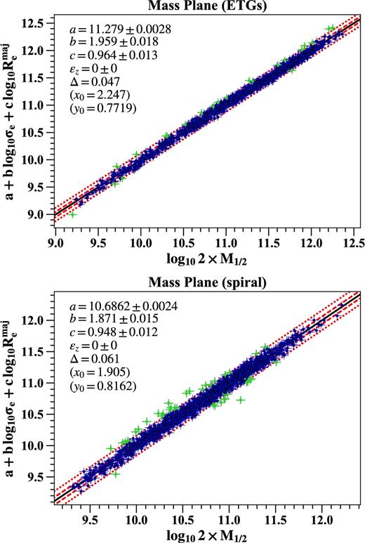
The edge-on view of the best-fitting mass plane for the ETGs (top) and the spiral galaxies (bottom) in our sample. The coefficients of the best-fitting plane a + b(x − x0) + c(y − y0) and the observed scatter Δ in z are shown at upper left of each panel. The red dashed lines show the 1σ (68 per cent) and 2.6σ (99 per cent). The outliers excluded from the fit by the LTS_PLANEFIT (Cappellari et al. 2013a) procedure are shown with green symbols.
As one can see, both ETGs and spiral galaxies are on a remarkably tight mass plane, with coefficients b and c close to the prediction from the virial theorem. This agrees with the results of b = 1.942, c = 0.991, and Δ = 0.077 in Cappellari et al. (2013b), and follow the virial theorem slightly better than the results of b = 1.67, c = 1.04, Δ = 0.059 from Scott et al. (2015) and α = 1.857, β = −1.279 in Auger et al. (2010), with α = 2, β = −1 being the prediction from the virial theorem in their formalism. The observed scatter Δ for spiral galaxies is 0.061, which is slightly larger than the value 0.047 for the ETGs. This is because the uncertainties in measuring the velocity dispersion, effective radius, and dynamical mass are larger for spiral galaxies due to the limited spectral resolution, the asymmetry of the galaxy and perturbation of the spiral arms. In the current data analysis pipeline for stellar kinematics, the extracted velocity dispersions under 50 km s−1 have larger scatters, and may be slightly overestimated due to the uncertainties of the instrumental resolution. This may account for the slightly larger deviation of the mass plane coefficients from the virial theorem for the spiral galaxies. The intrinsic scatters εz for both ETGs and spiral galaxies are consistent with being 0, until we reduce the error for the measured quantities in the fitting to 5 per cent (σe), 5 per cent (|$R_{\rm e}^{\rm maj}$|), and 3 per cent (M1/2). In the following sections, we use the ‘mass–size plane’ to refer to the projection of the mass plane along the σe direction. We choose this projection because it is close to face-on and the two axes have clear physical meanings (i.e. mass and size).
3.2 Stellar population on the mass–size plane
We estimate the stellar population properties for all the galaxies in our sample using the full spectrum fitting method described in Section 2.3. The distributions of the velocity dispersions, ages, metallicities, and stellar mass-to-light ratios of these galaxies on the mass–size plane are shown in Fig. 3. We use the python implementation3 (Cappellari et al. 2013b) of the two-dimensional Locally Weighted Regression (LOESS, Cleveland & Devlin 1988) method to obtain smoothed distributions, which are shown in Fig. 4. The velocity dispersions on the mass–size plane agree well with the prediction from the virial theorem, as indicated by the black dashed lines. The age, the metallicity, and the stellar mass-to-light ratio change systematically on the mass–size plane for both ETGs and spiral galaxies. The values increase roughly along the velocity dispersion direction, which trace the bulge mass fraction (Cappellari 2016). These systematic trends of the stellar population with velocity dispersion are consistent with a picture in which the bulge growth makes the population more metal rich and increases the likelihood for the star formation to be quenched (see fig. 23 of Cappellari 2016).
![Velocity dispersion σe, log Age, metallicity [Z/H], and stellar mass-to-light ratio M*/L (SDSS r band) distribution on the mass–size plane ($R_{\rm e}^{\rm maj}$ versus dynamical mass M1/2). Colours indicate the parameters as labelled at the top of each column. The results for early-type, spiral, and all galaxies are shown in the upper, middle, and bottom panels, respectively. In the bottom panels, coloured squares represent spiral galaxies and coloured circles represent ETGs. In each panel, dashed lines show lines of constant velocity dispersion: 50, 100, 200, 300, 400, and 500 km s−1 from left to right, as implied by the virial theorem. The magenta curve shows the zone of exclusion defined in Cappellari et al. (2013b).](https://oup.silverchair-cdn.com/oup/backfile/Content_public/Journal/mnras/476/2/10.1093_mnras_sty334/2/m_sty334fig3.jpeg?Expires=1750255047&Signature=Cli9M90Zy3F0KB98gmLRLxVcx5vpikLPpKnpcPl-Ty~OXso6C89vs6N5w1t03a-DyTmHDjcOGICuF2I3LwBQK0BtiSW2D~br-yGoLK2C~MTnohq7ftvU0vCPK6mjFRD1LzaBPOUIW~YuHMpJDp5BHg770kLpsemuC5KLFnlm-84rlBCVOvk1GAeA30~SuX6Qh1VaQbAgLcnfRq3qOhHCZPC-lCWH2IB5tRAzMJAtPobCOwyshPbPpHLVhjYJ-COvZZFQdXCoC4wXccTIqZTzPOwR1t6suc1xJXktgSIU8twyKmpiMQayXF0E1b3MxpDfvhYn2HvmBCmLR-vGJ31KHw__&Key-Pair-Id=APKAIE5G5CRDK6RD3PGA)
Velocity dispersion σe, log Age, metallicity [Z/H], and stellar mass-to-light ratio M*/L (SDSS r band) distribution on the mass–size plane (|$R_{\rm e}^{\rm maj}$| versus dynamical mass M1/2). Colours indicate the parameters as labelled at the top of each column. The results for early-type, spiral, and all galaxies are shown in the upper, middle, and bottom panels, respectively. In the bottom panels, coloured squares represent spiral galaxies and coloured circles represent ETGs. In each panel, dashed lines show lines of constant velocity dispersion: 50, 100, 200, 300, 400, and 500 km s−1 from left to right, as implied by the virial theorem. The magenta curve shows the zone of exclusion defined in Cappellari et al. (2013b).
![The same as Fig. 3, but with LOESS-smoothed σe, log Age, [Z/H], and M*/L.](https://oup.silverchair-cdn.com/oup/backfile/Content_public/Journal/mnras/476/2/10.1093_mnras_sty334/2/m_sty334fig4.jpeg?Expires=1750255047&Signature=hmOHWWon-2kHyqzlJlwROgfRgLt8NPGbto9FfQgh0x8Jr3y2MEjhf7U5oZvDWZ3qQwKGyo1tmS1TXpTdn39ex64ZGMSWsy8NtBspw3h7wZ~iyY9Pill6UC25alBtsmnXLVmJTDDBXuYixXz85-TBnybhC38jzwbfg6hVi-kNUoW4ASJeCQndIUBm~FG5Q0O7vM3p0t0fa5ewiUUBn0OmVNM3HQfoL3GBsBACfZGrSEKjg7OfWq~IkmehOyWmdQOgIIyE~OvT9EYpRtwXcjzrXMfgdGl~if-ByQli5ZMBbXVF~2rUUWhJZC7YMk9SfwmdW2DM72qly8Ccu~IIjj3psQ__&Key-Pair-Id=APKAIE5G5CRDK6RD3PGA)
The same as Fig. 3, but with LOESS-smoothed σe, log Age, [Z/H], and M*/L.
In a very recent work, Scott et al. (2017) showed similar results for ∼1300 galaxies with different morphologies from the SAMI IFU survey. Other than our sample being slightly larger (2110 versus 1300), our two studies differ in four aspects:
Their stellar population properties are derived from line indices, rather than full spectrum fitting as in our study.
They use stellar mass while we use dynamical mass.
They study the galaxy global properties only while we study both global properties and gradients in the stellar populations (see Section 3.3).
Finally, the two studies are based on quite different samples, observed with different IFUs, and analysed with different data pipelines.
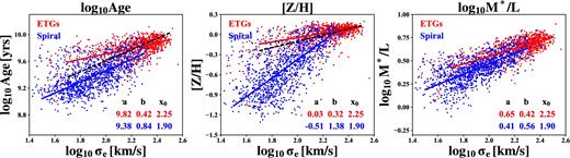
log Age (left), metallicity (middle), and stellar mass-to-light ratio (right) versus velocity dispersion. Early-type and spiral galaxies are shown with red and blue dots, respectively. The coloured solid lines show the best-fitting line a + b(x − x0) using the LTS_LINEFIT (Cappellari et al. 2013a) procedure. The coefficients are shown in the lower right in each panel while the black dashed line shows the results from Scott et al. (2017) for their galaxies in clusters.
3.3 Stellar population gradient on the mass–size plane
We use the method described in Section 2.3 to estimate the age, metallicity, and stellar mass-to-light ratio gradients for the galaxies in our sample. Similar to Figs 3 and 4, we show the distribution of these gradients on the mass–size plane in Figs 6 and 7. The systematic trends for the gradients are not as simple as the global properties which vary monotonically with the velocity dispersion as in Fig. 3, but there are several special features for the distribution of the population gradients on the mass–size plane:
Many galaxies with small size and mass have positive age and stellar mass-to-light ratio gradient (centre < outer), which may be due to the star formation in galaxy centre (Huang et al. 1996; Ellison et al. 2011; Oh, Oh & Yi 2012), while nearly all the galaxies with log102 × M1/2 > 11.2 have negative age and stellar mass-to-light ratio gradients. The age and the stellar mass-to-light ratio gradients for ETGs are correlated with galaxy mass.
The metallicity gradients for spiral galaxies increase (become more negative) with mass and size, while for ETGs, the metallicity gradients change with velocity dispersions. ETGs with higher and lower velocity dispersions have slightly shallower gradients.
Spiral galaxies with large size and mass have the steepest age, metallicity, and stellar mass-to-light ratio gradients. Although these galaxies are close to the massive ETGs on the mass–size plane, their gradient properties have significant differences. One can see a clear boundary between these two galaxy populations in Fig. 7, especially for the metallicity gradient. This may be due to the differences in their evolution histories, e.g. massive ETGs tend to have more mergers (Cappellari 2016). This also agree with the scenario that many of them are slow rotators (Graham et al. 2018), which are thought to be formed by mergers (Naab et al. 2014; Penoyre et al. 2017; Li et al. 2018).
![Age, metallicity, and stellar mass-to-light ratio gradient (Δlog Age, Δ[Z/H], and ΔM*/L) distribution on the mass–size plane. The gradients are defined in Section 2.3. A positive Δ value indicates a positive gradient, i.e. the central value is higher. Other labels are the same as in Fig. 3.](https://oup.silverchair-cdn.com/oup/backfile/Content_public/Journal/mnras/476/2/10.1093_mnras_sty334/2/m_sty334fig6.jpeg?Expires=1750255047&Signature=Y2-qgHRkwavZzcBOqV~dtTLHFi2U7EXrTk7PveA4-PtdUcceCPSmhYHVwJvQfb-rsmJotsk1sNCFtz1WCXkf2DYbGaFUHzoCKVjk6mh-M~ejLzCT0eEQyzOBUb7Yji5NDxdhLCv1WemICXV5yq4GgJCnfKcovfUeSL3YQsh3KDL-bU2W9NgkgnvaNx7-A5nl1f4b1UkV2hbXa2fJ0Vq76XP7vMNCuFTgYdHCKOw2l-24-Bm4HEtcV-6K4MLw8b8jOXnGbEN6Vu4SnJfB5Qb7FiLirMSR4VgQjmd36HIwYuIVVCD6SNUIIi9v6SuUp8RRbaZo0ilpgsij7qQUhfO6ag__&Key-Pair-Id=APKAIE5G5CRDK6RD3PGA)
![The same as Fig. 6, but with LOESS-smoothed Δlog Age, Δ[Z/H], and ΔM*/L.](https://oup.silverchair-cdn.com/oup/backfile/Content_public/Journal/mnras/476/2/10.1093_mnras_sty334/2/m_sty334fig7.jpeg?Expires=1750255047&Signature=TGCP-ZwUGB4K6IQIOGJ9UYiCMQgU00AObPrJuZV4Rbremv1I3rR6rHt4yAiEZTPk7tfvm9flHZbbQS0fXStsyc69RXXQakoex6q1uR9iUOhayIeCxRWF5XKFxDLEaB1jvi6SBwmjRcdVahd~JuGTx~dOmbFsz2dro53cGDQnvaejuQqUPXNtucjNWuSYrDZR4IxwoZWNDEGBclVUP~Pm8mNcfbhb62w7nJMaincrSV6r~NJAySlZYvnXi-rVYP4Eib-RiFc6Nuzka-zXsSyRDg1M-wICxbXwQeHNwL~hd57Lmc2wqlCqdTMxqwvNlrAmM~0N3eBu6ttFDFKlQHwVJg__&Key-Pair-Id=APKAIE5G5CRDK6RD3PGA)
The same as Fig. 6, but with LOESS-smoothed Δlog Age, Δ[Z/H], and ΔM*/L.
Here we note that our stellar mass-to-light gradients are based on the assumption of a constant Salpeter (1955) stellar IMF. The results will not be affected by the global variation of the IMF (e.g. Cappellari et al. 2012; Conroy & van Dokkum 2012; Li et al. 2017), but by a gradient of the IMF within galaxies (e.g. van Dokkum et al. 2017 for massive elliptical galaxies). The age and metallicity gradients will not be affected by the IMF.
In Fig. 8, we plot the histogram of the age, metallicity, and stellar mass-to-light ratio gradients and their relation with velocity dispersions. One can see that the age and the metallicity gradients peak around logσe = 2.0 (especially for metallicity gradients), which roughly corresponds to the critical mass ∼3 × 10¹⁰ M⊙ of the break in the mass–size relation (Cappellari 2016), below which no fully passive ETGs exist. The same critical mass is also shown in Kauffmann et al. (2003). This agrees well with the results in Spolaor et al. (2009), Tortora et al. (2010), Kuntschner et al. (2010), and Kuntschner (2015), but is slightly different from the results in Goddard et al. (2017), which did not show a clear decrease of the metallicity gradients with increasing stellar masses. The galaxies in our sample occupy similar region of the metallicity–velocity dispersion relationship with the simulated galaxies in Hopkins et al. (2009). We also construct Figs 6, 7, and 8 with intermediate Sérsic index (2–3) galaxies excluded, and find no significant differences from the main sample.
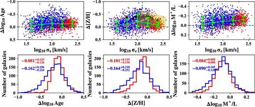
Top: gradients of log Age (left), metallicity (middle), and stellar mass-to-light ratio (right) versus velocity dispersion. Early-type and spiral galaxies are shown with red and blue dots, respectively. The green error bars show the median and scatter of all the galaxies in each bin, calculated as the 16th, 50th, and 84th percentiles. In the middle panel, black stars are the results from Kuntschner (2015), the pink dashed line shows the trend from Spolaor et al. (2009) while the yellow shaded region shows the galaxy distribution from the simulation Hopkins et al. (2009). Bottom: distribution of the log Age (left), metallicity (middle), and stellar mass-to-light ratio (right) gradients for the early-type and spiral galaxies. The medians and 1σ scatters of the distributions are shown in each panel.
In Fig. 9, to visually illustrate and confirm the reality of the statistical results of Figs 6 and 7, we show the metallicity profiles between Re/8 and 1Re of some galaxies with the best data qualities on the mass–size plane. The selected galaxies have more than 400 Voronoi bins with S/N greater than 30 for the top four rows in Fig. 9, and more than 200 Voronoi bins for the bottom row because small galaxies have lower data qualities. The spiral galaxies with large size and mass have very steep metallicity gradients, while the gradients for massive elliptical galaxies are much shallower. The morphology and the other measured properties for the galaxies in our sample are listed in Table A1.
![Metallicity profiles ([Z/H] versus log10 R/Re) for the selected high S/N galaxies in different regions of the mass–size plane. Blue lines are the profiles for the spiral galaxies, red lines are for the ETGs. In each panel, the black solid lines represent the gradient values of 0, −0.1, −0.3, and −0.5, respectively. All the panels have the same scales as shown in the upper left panel. All the profiles have been shifted to be 0 at Re/8.](https://oup.silverchair-cdn.com/oup/backfile/Content_public/Journal/mnras/476/2/10.1093_mnras_sty334/2/m_sty334fig9.jpeg?Expires=1750255047&Signature=BUxJX~VmF1DJ68Ow8riiO5L3FgDFpJUleqRa8dFvcD3Q-X1WG3j0GqfUcND46RmAGs0sLCddI~xgTt6b5A8P6sc1D-M28Odpj-evwmB6nX9fupnmYZg0ooxP0lktAq3TnGR3O4cWDC7K4DzIsZO4F8AmgkxbJKhl7L08RshZSozfOY4r8nclO-rzM6AXHwz2gILs-5tOkOR~bwVgIJYi1gbJhqEXAL9gfiBKpw5-uzImDoL7W4~Agtd40CCI6gBHI6Sfgz21fOyWhWAWnPWifp4vWgqaK7KuM73eeTRirOd1X5k6ugZCheVbN5VCDPyGpay8J5WcYzwVtjj-vDkf3A__&Key-Pair-Id=APKAIE5G5CRDK6RD3PGA)
Metallicity profiles ([Z/H] versus log10 R/Re) for the selected high S/N galaxies in different regions of the mass–size plane. Blue lines are the profiles for the spiral galaxies, red lines are for the ETGs. In each panel, the black solid lines represent the gradient values of 0, −0.1, −0.3, and −0.5, respectively. All the panels have the same scales as shown in the upper left panel. All the profiles have been shifted to be 0 at Re/8.
4 CONCLUSIONS
JAM and full spectrum fitting have been used to study the mass plane scaling relationship and the distribution of the stellar population properties on a inclined projection of the mass plane, i.e. the mass–size plane. The galaxies used in this study are from the MaNGA DR14 sample, which is currently the largest IFU sample including both early- and late-type galaxies.
Below we summarize our main results:
Both early-type and spiral galaxies are on a remarkably tight mass plane, with the best-fitting coefficients close to the predicted values from the virial theorem. This extends the previous result for ETGs population to the whole galaxy population.
The stellar population properties (i.e. age, metallicity, and stellar mass-to-light ratio) of the galaxies in our sample vary systematically on the mass–size plane along roughly the velocity dispersion direction. The stellar population of the galaxies with higher velocity dispersion are older and more metal rich, which are consistent with a picture in which the bulge growth makes the population more metal rich and increases the likelihood for the star formation to be quenched (Cappellari 2016).
The gradients of age and stellar mass-to-light ratio could be positive (centre < outer) for low-mass galaxies, while most massive galaxies have negative gradient.
The metallicity–velocity dispersion relation shows a clear peck around logσe ≈ 2.0, which corresponds to the critical mass ∼3 × 10¹⁰ M⊙ of the break in the mass–size relation (Cappellari 2016), below which no fully passive ETGs exist.
The distribution of the population gradients on the mass–size plane shows a clear boundary between massive spiral and early-type galaxies. Spiral galaxies with large size and mass have the steepest gradients. In contrast, the massive ETGs located in similar region have shallower gradients. This may be due to differences in their evolution histories, e.g. mergers.
The trends we see in this work, particularly the gradients shown in Figs 6 and 7, are puzzling and warrant further studies. Observationally, these trends are still subject to the age-metallicity degeneracy and the scatters are still somewhat high. Theoretically, the spatial resolutions in numerical simulations and the treatments of physical processes, such as the chemical enrichment and feedback processes, will affect the final predictions of the stellar populations and their gradients. For example, according to Taylor & Kobayashi (2017) the metallicity gradients are affected by the initial steep gradients from gas-rich assembly, passive evolution by star formation and accretion at outskirts and flattening by mergers (major and minor). In reality, all these processes may be operating at the same time, and it will take further efforts to decode the information we assembled here. More detailed comparisons with high-resolution cosmological simulations such as Illustris (Vogelsberger et al. 2014a,b) and EAGLE (Schaller et al. 2015) may be a fruitful next step.
Acknowledgements
We thank Harald Kuntschner for providing the stellar population profiles for the seven selected galaxies from the ATLAS3D survey and the referee for helpful comments. MC acknowledges support from a Royal Society University Research Fellowship. We performed our computer runs on the Zen high performance computer cluster of the National Astronomical Observatories, Chinese Academy of Sciences (NAOC), and the Venus server at Tsinghua University. This work was supported by the National Science Foundation of China (Grant No. 11333003, 11390372 to SM). This research made use of Marvin, a core python package and web framework for MaNGA data, developed by Brian Cherinka, José Sánchez-Gallego, and Brett Andrews (MaNGA Collaboration, 2017).
Funding for the Sloan Digital Sky Survey IV has been provided by the Alfred P. Sloan Foundation, the U.S. Department of Energy Office of Science, and the Participating Institutions. SDSS-IV acknowledges support and resources from the Center for High-Performance Computing at the University of Utah. The SDSS web site is www.sdss.org.
SDSS-IV is managed by the Astrophysical Research Consortium for the Participating Institutions of the SDSS Collaboration including the Brazilian Participation Group, the Carnegie Institution for Science, Carnegie Mellon University, the Chilean Participation Group, the French Participation Group, Harvard-Smithsonian Center for Astrophysics, Instituto de Astrofísica de Canarias, The Johns Hopkins University, Kavli Institute for the Physics and Mathematics of the Universe (IPMU) / University of Tokyo, Lawrence Berkeley National Laboratory, Leibniz Institut für Astrophysik Potsdam (AIP), Max-Planck-Institut für Astronomie (MPIA Heidelberg), Max-Planck-Institut für Astrophysik (MPA Garching), Max-Planck-Institut für Extraterrestrische Physik (MPE), National Astronomical Observatories of China, New Mexico State University, New York University, University of Notre Dame, Observatário Nacional / MCTI, The Ohio State University, Pennsylvania State University, Shanghai Astronomical Observatory, United Kingdom Participation Group, Universidad Nacional Autónoma de México, University of Arizona, University of Colorado Boulder, University of Oxford, University of Portsmouth, University of Utah, University of Virginia, University of Washington, University of Wisconsin, Vanderbilt University, and Yale University.
Footnotes
Available from http://purl.org/cappellari/software
Available from http://purl.org/cappellari/software
REFERENCES
SUPPORTING INFORMATION
Supplementary data are available at MNRAS online.
Please note: Oxford University Press is not responsible for the content or functionality of any supporting materials supplied by the authors. Any queries (other than missing material) should be directed to the corresponding author for the article.
APPENDIX : EXAMPLE DATA TABLE
Properties of all the galaxies in the sample.
| MaNGA ID | Morphology | log10 σe | log10 M1/2 | |$\log _{10} \,R_{\rm e}^{\rm maj}$| | log10 Age | [Z/H] | log10M*/Lr | Δlog10 Age | Δ[Z/H] | Δlog10 M*/Lr |
|---|---|---|---|---|---|---|---|---|---|---|
| (km s−1) | (M⊙) | (kpc) | (yr) | (M⊙/L⊙r) | ||||||
| (1) | (2) | (3) | (4) | (5) | (6) | (7) | (8) | (9) | (10) | (11) |
| 1-320664 | S | 2.17 | 10.66 | 0.76 | 9.95 | 0.06 | 0.75 | − 0.15 | 0.14 | − 0.08 |
| 1-321069 | E | 2.37 | 11.48 | 1.07 | 9.80 | 0.14 | 0.66 | − 0.12 | − 0.05 | − 0.12 |
| 1-235587 | E | 2.04 | 10.27 | 0.50 | 9.66 | 0.06 | 0.54 | 0.04 | − 0.33 | − 0.04 |
| 1-320677 | E | 2.27 | 11.41 | 1.14 | 9.70 | 0.12 | 0.60 | − 0.38 | 0.18 | − 0.30 |
| 1-235576 | S | 2.10 | 10.82 | 0.75 | 9.74 | − 0.57 | 0.68 | − 0.04 | 0.45 | − 0.14 |
| 1-235530 | E | 2.22 | 10.53 | 0.41 | 9.90 | 0.07 | 0.73 | − 0.33 | − 0.15 | − 0.28 |
| 1-235398 | S | 2.10 | 10.67 | 0.78 | 9.71 | − 0.21 | 0.57 | 0.13 | − 0.10 | 0.06 |
| 1-320606 | S | 1.86 | 10.46 | 0.93 | 9.04 | − 0.86 | 0.21 | − 0.43 | − 0.55 | − 0.31 |
| 1-321074 | E | 2.27 | 11.04 | 0.83 | 9.64 | 0.15 | 0.56 | − 0.10 | − 0.09 | − 0.10 |
| 1-235582 | E | 1.84 | 9.92 | 0.58 | 9.33 | 0.07 | 0.30 | 0.31 | − 0.20 | 0.26 |
| 1-320584 | E | 2.47 | 11.70 | 1.08 | 9.94 | 0.12 | 0.77 | − 0.19 | − 0.06 | − 0.16 |
| 1-235611 | S | 2.06 | 11.00 | 1.11 | 9.56 | − 0.15 | 0.56 | − 0.68 | − 0.52 | − 0.39 |
| 1-320655 | E | 2.37 | 11.25 | 0.78 | 9.85 | 0.12 | 0.70 | − 0.23 | 0.00 | − 0.16 |
| 1-24092 | E | 2.13 | 10.37 | 0.35 | 9.01 | − 0.73 | 0.42 | 0.08 | − 0.28 | 0.35 |
| 1-23979 | E | 2.00 | 10.25 | 0.53 | 9.59 | − 0.10 | 0.53 | 0.02 | − 0.22 | − 0.01 |
| 1-24099 | E | 2.07 | 10.23 | 0.38 | 9.68 | 0.10 | 0.57 | − 0.11 | − 0.17 | − 0.08 |
| 1-23929 | S | 1.80 | 10.25 | 0.83 | 9.34 | − 0.52 | 0.41 | − 0.41 | − 0.12 | − 0.08 |
| 1-24368 | S | 1.72 | 9.96 | 0.77 | 9.19 | − 0.76 | 0.20 | − 0.14 | 0.06 | − 0.33 |
| 1-24354 | S | 1.75 | 9.87 | 0.51 | 9.83 | − 0.26 | 0.56 | − 0.14 | 0.10 | − 0.07 |
| 1-595027 | S | 2.05 | 10.72 | 0.90 | 9.24 | − 0.75 | 0.48 | − 0.25 | − 0.72 | − 0.04 |
| 1-595093 | S | 2.17 | 10.99 | 1.03 | 9.66 | − 0.02 | 0.64 | − 0.40 | − 0.13 | − 0.19 |
| 1-24018 | E | 2.11 | 10.58 | 0.71 | 9.78 | 0.07 | 0.64 | − 0.11 | − 0.22 | − 0.14 |
| 1-23891 | S | 2.20 | 10.82 | 0.78 | 9.80 | 0.03 | 0.66 | − 0.26 | 0.06 | − 0.18 |
| 1-24148 | S | 2.10 | 10.61 | 0.71 | 9.81 | 0.05 | 0.69 | − 0.19 | 0.10 | − 0.13 |
| 1-25937 | S | 2.22 | 11.34 | 1.22 | 9.70 | − 0.00 | 0.60 | − 0.36 | − 0.39 | − 0.25 |
| 1-25911 | E | 2.37 | 11.57 | 1.14 | 9.72 | 0.09 | 0.59 | − 0.24 | − 0.09 | − 0.23 |
| 1-24124 | S | 1.68 | 9.74 | 0.53 | 9.43 | 0.04 | 0.43 | 0.06 | 0.07 | − 0.02 |
| 1-115062 | E | 2.12 | 10.02 | 0.00 | 9.80 | 0.11 | 0.65 | − 0.00 | 0.04 | − 0.02 |
| 1-114928 | E | 2.24 | 10.76 | 0.67 | 9.91 | − 0.02 | 0.71 | − 0.12 | − 0.31 | − 0.19 |
| 1-115128 | S | 1.99 | 10.70 | 0.94 | 9.23 | − 0.59 | 0.34 | − 0.16 | − 0.50 | − 0.15 |
Column (1): The MaNGA ID of the galaxy. Column (2): Galaxy morphology. E for ETGs, S for spiral galaxies. Column (3): Velocity dispersion within 1Re, as defined in equation (2). Column (4): Enclosed total mass within three-dimensional half-light radius from dynamical model, M1/2. Column (5): Major axis of the half-light isophote for the best-fitting MGE model. Column (6): Mean logAge within the effective radius. Column (7): Mean metallicity within the effective radius. Column (8): Mean stellar mass-to-light ratio within the effective radius in SDSS r band. Column (9): Age gradient. Column (10): Metallicity gradient. Column (11): Stellar mass-to-light ratio gradient in SDSS r band. Please see the journal website for the complete table.
