


Abstract
We performed an analysis of the main theoretical uncertainties that affect the radius of low- and very-low-mass stars predicted by current stellar models. We focused on stars in the mass range 0.1–1 M⊙, on both the zero-age main sequence (ZAMS) and on 1, 2, and 5 Gyr isochrones. First, we quantified the impact on the radius of the uncertainty of several quantities, namely the equation of state, radiative opacity, atmospheric models, convection efficiency, and initial chemical composition. Then, we computed the cumulative radius error stripe obtained by adding the radius variation due to all the analysed quantities. As a general trend, the radius uncertainty increases with the stellar mass. For ZAMS structures the cumulative error stripe of very-low-mass stars is about ±2 and ±3 per cent, while at larger masses it increases up to ±4 and ±5 per cent. The radius uncertainty gets larger and age dependent if isochrones are considered, reaching for M ∼ 1 M⊙ about +12(−15) per cent at an age of 5 Gyr. We also investigated the radius uncertainty at a fixed luminosity. In this case, the cumulative error stripe is the same for both ZAMS and isochrone models and it ranges from about ±4 to +7 and +9(−5) per cent. We also showed that the sole uncertainty on the chemical composition plays an important role in determining the radius error stripe, producing a radius variation that ranges between about ±1 and ±2 per cent on ZAMS models with fixed mass and about ±3 and ±5 per cent at a fixed luminosity.
1 INTRODUCTION
In recent years, accurate measurements of stellar radii for low- and very-low-mass stars have become available both for single stars, through interferometric measurements, and for eclipsing binary systems (see e.g. Ségransan et al. 2003; Berger et al. 2006; Mathieu et al. 2007; Demory et al. 2009; Torres, Andersen & Giménez 2010; Boyajian et al. 2012a,b).
The continuously growing sample of stars for which accurate mass and radius measurements are available suggests that stellar models tend to systematically underestimate the radius of low-mass (LM) and very-low-mass (VLM) stars by about 3–20 per cent, depending on the stellar mass (see e.g. Torres & Ribas 2002; Chabrier et al. 2005; Berger et al. 2006; Morales et al. 2009; Boyajian et al. 2012b; Spada et al. 2013; Torres 2013). Such a sizeable disagreement prompted a renewed interest on theoretical models of low-mass stars and on their evolution.
In spite of the significant improvement of stellar evolution computations in the last decades, models are still affected by uncertainties coming from the adopted input physics [i.e. equation of state (EOS), radiative opacity, boundary conditions (BCs)], initial chemical composition, and from the still oversimplified treatment of the convection in superadiabatic regimes (i.e. the largely adopted mixing length theory, MLT; Böhm-Vitense 1958). This last point is particularly important for stars with deeper superadiabatic envelopes (i.e. M ≳ 0.3–0.4 M⊙, for solar chemical composition). The discrepancy between the expected and observed mass–radius relation leaded also to investigate possible non-standard mechanisms that might produce the observed radius inflation.
From the observational point of view, Kraus et al. (2011) claimed a possible correlation between the radius inflation and the orbital period of binary stars. They found that short period (<1.5 d) tidally locked stars seem to exhibit larger radius than longer period counterparts. However, the correlation is still debated (Feiden & Chaboyer 2012a). Moreover, Spada et al. (2013) found similar levels of radius inflation in both single and binary stars.
Systems with inflated radii tend to show also an high level of magnetic activity and/or spot coverage (Torres & Ribas 2002; Chabrier, Gallardo & Baraffe 2007; López-Morales 2007; Ribas et al. 2008; Stassun et al. 2012; Feiden & Chaboyer 2013; Somers & Pinsonneault 2015), although a clear correlation has not yet been found (Mann et al. 2015). Moreover, the presence of stellar spots alters also the stellar properties derived from the light-curve analysis of binary systems (see e.g. Morales et al. 2010; Windmiller, Orosz & Etzel 2010).
The effect of a relatively strong magnetic field in stellar models has been recently investigated in several papers (Chabrier et al. 2005; Feiden & Chaboyer 2012b, 2013, 2014b, and references therein). Feiden and collaborators showed that the introduction of a magnetic field acts to reduce the convection efficiency in the external superadiabatic region. The magnetic field strength can be tuned to improve the agreement between data and models, at least in stars with radiative cores and convective envelopes (Feiden & Chaboyer 2013). On the other hand, in the case of fully convective stars, extremely large and unrealistic magnetic fields are required. As such, magnetic field is unlikely to be the sole mechanism acting to inflate the radius (Feiden & Chaboyer 2014a,b, 2014c). Interestingly, Feiden & Chaboyer (2013) showed also that the main effect of magnetic convection inhibition can be reproduced, in standard models with no magnetic fields, by simply changing the mixing length parameter (αML). In particular they showed that a value of αML much lower than the solar calibrated one allows to mimic the main effects of the presence of an internal magnetic field. Models of main sequence (MS) and pre-MS low-mass stars with reduced external convection efficiency (αML ≤1) show, in some cases, a better agreement with observational data (i.e. radius or surface lithium abundance; see e.g. Chabrier, Gallardo & Baraffe 2007; Tognelli, Degl’Innocenti & Prada Moroni 2012).
Another aspect related to the presence of strong magnetic fields is surface stellar spots phenomenon. The presence of spots with long enough lifetime, which depends on thermal time-scales of the convective envelope (Spruit & Weiss 1986), might lead to a reduction of surface energy flux, due to the presence of spotted cooler regions, thus inducing a radius inflation and a change in the expected colours [spectral energy distribution (SED)]. Depending on the assumptions made on the spots (i.e. their depth, temperature, and coverage fraction) a radius variation up to about 10 per cent can be obtained (depending on stellar mass and age; see e.g. Somers & Pinsonneault 2015). Chabrier et al. (2007) showed that models that account for both spots and magnetic convection inhibition lead to a better agreement with observed low-mass stars radii.
Recently Chen et al. (2014) were able to get a good agreement between models and data for low-mass stars by modifying the temperature profile in the atmospheric models used as BC for the computation of stellar models. They suggested that a possible reason for part of the disagreement between the observed and predicted mass–radius relation might be found in the still not satisfactory synthetic atmospheric structures used to obtain outer BCs for stellar models. However, such models systematically underestimate the effective temperature of VLM and LM stars in clusters, as shown by Randich et al. (2017).
The aim of this paper is to focus on the prediction of standard models (i.e. without the presence of magnetic fields, spots, or rotation) and to give a quantitative estimation of the actual uncertainty in the predicted stellar radius, due to the uncertainty in the adopted input physics, initial chemical composition, and convection efficiency. As a result we obtained a cumulative error stripe in the predicted radius, when all the uncertainty sources are accounted for at the same time.
The paper is structured as it follows. In Section 2 we introduce the standard set of models. Then, we analyse the contribution to the radius uncertainty due to the errors of several adopted input physics in Section 3 and due to the uncertainty in the adopted initial chemical composition in Sections 4. In Section 5 the cumulative error stripe for the stellar radius computed, by adding all the contribution to the radius uncertainty analysed in the paper, is presented. In Section 6 we summarize the main results of this work.
2 THE MODELS
We computed LM and VLM stellar models using the Pisa version of the franec code (prosecco; Tognelli, Prada Moroni & Degl’Innocenti 2011; Dell’Omodarme et al. 2012), described in details in Tognelli, Prada Moroni & Degl’Innocenti (2015a) and Tognelli et al. (2015b). Here we briefly recall the main input physics relevant for the present analysis. We adopted opal 2005 radiative opacities in the interior for log T(K) ≥ 4.5 extended with the Ferguson et al. (2005, hereafter F05) at lower temperatures. Both the opal and the F05 opacities are computed for the Asplund et al. (2009, hereafter AS09) solar mixture. The EOS has been obtained using the opal EOS 2006 (Rogers & Nayfonov 2002) as reference, extended by the scvh95 EOS (Saumon, Chabrier & van Horn 1995) in the low temperature–high pressure regime. The outer BCs have been extracted from the non-grey Allard, Homeier & Freytag (2011, hereafter AHF11)1 atmospheric structures. The atmosphere adopts the same heavy elements mixture (i.e. AS09) and mixing length parameter (i.e. αML = 2.0) used in the interiors. To be noted that αML = 2.0 is the solar calibrated value we obtained with our models.
Besides the reference value αML = 2.00, we also computed models for a much lower mixing length parameter value, namely αML = 1.00, corresponding to a much less efficient superadiabatic convection. To this regard, Chabrier et al. (2007) showed that the reduction of superadiabatic convection efficiency might partially reduce the disagreement level between the predicted and observed radii of low-mass stars. The availability of two sets of stellar tracks with significantly different αML values allows us to investigate whether the theoretical uncertainty on the stellar radius depends on such a poorly constrained parameter.
For the standard set of stellar tracks we chose [Fe/H] = +0.0, which corresponds to an initial helium abundance Y = 0.274 and metallicity Z = 0.013 by assuming the AS09 solar heavy-element mixture.
The stellar models cover the mass range [0.1, 1.0] M⊙, with a variable mass spacing of 0.02 M⊙ for M ∈ [0.1, 0.5] M⊙ and 0.05 M⊙ for M > 0.5 M⊙. From the stellar tracks we then built the zero-age main sequence (ZAMS), identified as the sequence of models of different mass whose central hydrogen abundance has been reduced by 0.02 per cent with respect to the initial one. Although this is not the rigorous definition of ZAMS, we checked that it is a good approximation, with the advantage of being easily and consistently implementable in all the mass range we analysed.2 We recall that the models on ZAMS do not share the same age. Indeed, stars with a different mass ignite the central hydrogen burning at different ages, and the lower is the stellar mass, the larger is the ZAMS age. In particular, in the selected mass range, the ZAMS sequence is populated by models with ages from 50 Myr (∼1.0 M⊙) up to about 5 Gyr (∼0.1 M⊙). To investigate the uncertainty in the stellar radius at fixed age, isochrones for three ages, namely 1, 2, and 5 Gyr, have been calculated.
We show in Fig. 1 a comparison between the theoretical stellar radius as a function of the mass obtained from our reference models on the ZAMS and on the 1, 2, and 5 Gyr isochrone sequences.
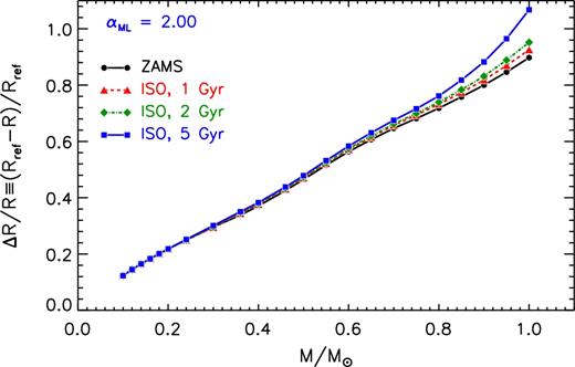
Stellar radius (in solar units) as a function of the mass for our reference set of models located on the ZAMS (black solid line) and on 1, 2, and 5 Gyr isochrones (coloured lines).
3 UNCERTAINTY IN THE ADOPTED INPUT PHYSICS
As a first step of our analysis, we quantified the uncertainty in the stellar radius caused by the uncertainty in the adopted input physics by varying, separately, each of the main quantities relevant for the stellar evolution up to the ZAMS/MS phase.
We followed two approaches when analysing the effect of one perturbed quantity on the stellar radius. In one case, we simply take the relative difference between the radius prediction – at a given mass – of the reference set and of the set with one perturbed quantity. The latter have been computed by changing/perturbing a single input physics and keeping the other quantities to their reference values. In the second approach, we performed a new solar calibration of the mixing length parameter in the models with the perturbed input physics. This second case deserves a brief explanation.
As previously mentioned, the reference set of models adopted a solar calibrated mixing length parameter (αML⊙). Such a value has been obtained by requiring that a 1 M⊙ stellar model, at the age of the Sun, must reproduce simultaneously the radius, luminosity, and surface (Z/X) of the Sun. The solar calibration is performed by tuning three initial parameters, namely αML⊙, the initial helium Y⊙, and the metal Z⊙ content, which affect the solar luminosity, radius, and surface (Z/X). However, in the present analysis we did not fully use the solar calibrated values, in the sense that the initial chemical composition adopted for the computation is fixed and derived assuming [Fe/H] = 0 (see Section 4) and it is not that resulting from the solar calibration. Thus, here with solar calibration we mean models computed with only the solar calibrated αML.
In this second approach we thus performed the solar calibration for models with the perturbed input physics, to assure that the 1 M⊙ model reproduces the solar characteristics. This approach is different from the first one where no calibration is done. In some cases and for masses close to the 1 M⊙, it might happen that the differences between the reference set of models and that with the perturbed input physics can be partially counterbalanced by the recalibrated αML⊙ value.
In the following, we will discuss the results of adopting these two approaches in each analysed case.
3.1 Outer boundary conditions: atmospheric models
The outer BCs necessary to integrate the stellar structure equations consist of the pressure Pbc ≡ P(τbc) and temperature Tbc ≡ T(τbc) – obtained from an atmospheric model – at a given optical depth τbc, corresponding to the point where the atmosphere matches the interior of the star (defined as the region where τ > τbc). When considering the uncertainty due to the adopted BCs, two aspects have to be analysed: (1) the atmospheric model used to obtain Pbc and Tbc; and (2) the adopted τbc value.
Concerning the first point, at the moment no estimation of the uncertainty on the results of atmospheric model computations is available. As such, a firm evaluation of the uncertainty in the adopted Pbc and Tbc values cannot be consistently obtained. A possible way to estimate the effect of the BCs on the models is to compare the results obtained adopting different atmospheric structures in the stellar evolutionary code. To do this we used the BCs provided by two detailed (non-grey) sets of atmospheric models, namely the Brott & Hauschildt (2005, hereafter BH05) and the Castelli & Kurucz (2003, hereafter CK03). We also computed a set of models using the still largely used Krishna Swamy (1966, hereafter KS66) atmosphere that adopts an empirical T = T(Teff, τ) relation calibrated on the Sun. In the latter case the atmospheric structure is calculated directly inside the stellar evolutionary code, with exactly the same input physics used for the computation of the interior.
The top panel of Fig. 2 shows the relative radius variation due to the adoption of the quoted BCs instead of the reference AHF11 for ZAMS models, at a fixed value of the stellar mass. To better understand the radius variation due to the BCs, more details are required. The BH05 have been computed by means of the same atmospheric code (phoenix; see e.g. Hauschildt & Baron 1999) used to compute our reference set of atmospheres (AHF11), but the latter has been recently upgraded to better describe the atmospheric structure of LM and VLM stars. The two sets of phoenix atmosphere models differ in several aspects: (1) updated solar mixture (metal abundances), which has a crucial role in determining the opacity in the atmosphere (molecules/dust); (2) updated opacity lines (especially for H2O, CH4, NH3, and CO2); and (3) updated treatment of cloud/dust formation/diffusion (important for cool atmospheres, below 2600–2700 K). The global effect of all the differences between the two sets of atmospheric structures is to produce a radius variation that depends on the stellar mass. For M ≲ 0.5 M⊙ the radius variation is very small and less than 1 per cent, while it progressively increases reaching about +2 per cent at 1 M⊙.

As previously stated, one of the differences between the AHF11 and the BH05 atmosphere is the adopted solar mixture. The recent AHF11 atmospheric structures are computed using the AS09 – which is consistent with the interior calculation – while the BH05 used the Grevesse & Noels (1993, hereafter GN93). It is evident that the adoption of the BH05 BCs produces an inconsistency between the interior and atmospheric structures, at least for what concerns the metals abundances. Unfortunately, the BH05 are not available for the AS09 mixture, so we cannot analyse the effect of the mixture in this case. However, the AHF11 have been made available also for the GN93 mixture (AHF11+GN93 set of models in Fig. 2). This allows us to estimate the effect of a mixture change in the atmosphere, keeping fixed that in the interior (AS09). As clearly visible in figure, the radius variation due to the adoption of a different solar mixture in the atmosphere is very small in VLM stars, below 0.6–0.7 M⊙, and it reaches a plateau at about 1 per cent for larger masses. It is interesting to compare the result found for the BH05 and the AHF11+GN93 models. The two cases show a very similar behaviour, but the two sets of models are shifted by an almost constant offset, which indicates that part of the effect on the radius is caused by the different mixture used in the interior and in the atmosphere, while the remaining part has to be found in the other differences between the two adopted atmospheric structures, as discussed above.
It is interesting to analyse also the effect of adopting a totally different atmospheric models. To do this we showed also the comparisons with the atlas code atmosphere (Kurucz 1970), in the CK03 configuration. To be noted that the CK03 are available only for Teff ≥ 3500 K, which in our case corresponds to about 0.36 M⊙, in ZAMS. From Fig. 2 it is evident that the maximum radius variation strongly depends on the stellar mass, reaching about −1.5 per cent for M ≲ 0.4 M⊙ and +1.5 per cent at about 0.7 M⊙. The atlas code is different from the phoenix one in many aspects, so it is difficult to clearly identify the discrepancy sources. Some of possible relevant differences might be found in (1) the opacity sampling/calculation, (2) opacity lines list, (3) solar mixture (i.e. Grevesse & Sauval 1998, in CK03), and (4) αML (1.25 in CK03). All these quantities have a role in determining the final BCs, but the detailed analysis of their individual impact in the models is beyond the scope of the present work.
We also showed the effect on the radius of adopting the semi-empirical solar calibrated KS66 atmosphere. We emphasize that such an atmospheric model is a too rough approximation for VLM stars, being calibrated on the Sun. However, grey T(τ) hydrostatic atmosphere had been adopted in the past in the regime of LM and VLM stars to compute still used stellar evolutionary libraries (e.g. D’Antona & Mazzitelli 1994, 1997). We thus used the KS66 as representative of this class of stellar models. The KS66 BCs produce the largest radius variation in almost the whole analysed mass range, which reaches about −3 per cent. To be noted that in the KS66 models the radius is systematically larger than the reference one and the resulting models are cooler.
The bottom panel of Fig. 2 shows the relative radius variation obtained by adopting the same BCs discussed above, but for models on the 1, 2, and 5 Gyr isochrones. In almost all the cases, the radius change is similar to that obtained for the ZAMS in the whole selected mass range, with no evident dependence on the age. Only in the case of the KS66 BCs, the radius variation slightly increases with the age for masses larger than about 0.8 M⊙.
These results have been obtained adopting αML = 2.00. We performed the same analysis using αML = 1.00, to evaluate the dependence on αML. The adoption of the non-grey BCs (i.e. BH05, CK03, or AHF11+GN93) produces a radius variation almost identical to that obtained in the models with αML = 2.00. On the contrary, the use of the KS66 results in a larger surface radius variation that reaches values about 1.5 times larger than those obtained in the models with αML = 2.00 in both the ZAMS and the isochrone case, but only for M ≳ 0.3 M⊙. We want to precise that, when changing the αML value, we actually change it in the interiors (τ > τbc), as in the non-grey atmosphere αML is fixed. Thus, we do not properly account for the effect of αML in the whole structure. Moreover, the dependence of the KS66 models on the adopted αML probably resides in the fact that KS66 adopt τbc = 2/3, as suggested in the original paper, instead of τbc = 10 (our reference in non-grey models). This means that when the KS66 BCs are used, the interior calculations extend to lower values of τ, thus covering a portion of the star that in non-grey BCs is incorporated in the atmosphere and thus independent of the value of αML used for the interiors. Such most external regions can be superadiabatic, especially at progressively larger values of the stellar mass analysed here, and sensitive to the adopted αML. Such an effect is almost inconsequential in VLM, which have adiabatic external layers that extend to the bottom of the atmosphere. This qualitatively explains the dependence of the KS66 models to the adopted αML, as the mass increases.
We also analysed the radius change due to the adoption of different BCs when the solar calibration is performed for each set of perturbed models. To be noted that the outer BCs mainly affect the radius of the star. As a consequence, the solar calibration results in the same initial Y⊙ and Z⊙ values but in different αML⊙. In particular we obtained the following values: αML⊙ = 1.74 for BH05, αML⊙ = 1.88 for AHF11+GN93, αML⊙ = 1.95 for CK03, and αML⊙ = 2.25 for KS66. The constancy of the initial chemical composition means that all the radius change due to the use of different BCs is counterbalanced in 1 M⊙ model by the adoption of a properly tuned αML⊙. Thus, around 1 M⊙ the radius change is cancelled if the solar calibrated αML⊙ is adopted. However, star of different masses are sensitive in a different way to the αML, so we do not expect that the solar calibrated αML⊙ is able to counterbalance the radius change in all the selected mass range.
Fig. 3 shows the radius variation in ZAMS induced by the adopted BCs for solar calibrated αML⊙ values. It is clearly visible that the radius change is not affected by the adopted αML⊙ value for M ≲ 0.6 M⊙, while for larger masses, as expected, the adoption of a solar value of αML progressively reduces the radius variation.

As in Fig. 2 but for solar calibrated αML values.
3.2 Outer boundary conditions: τbc
As anticipated in the previous section, the BCs are also affected by the choice of τbc. This quantity is freely chosen and generally it assumes values in the interval 2/3 ≲ τbc ≲ 100 (see e.g. table 2 in Tognelli et al. 2011). The choice of τbc is not trivial. Here we limit to recall that in the computations of the stellar interior (i.e. for τ > τbc) the diffusive radiative approximation has to be fulfilled. To this regard, Morel et al. (1994) showed that a value of τbc ≥ 10 should be adopted (see also Trampedach et al. 2014). To test the dependency of the predicted radius on τbc, we computed models for three values of τbc, namely 2/3, 10 (our reference), and 100 (with the reference AHF11 atmosphere). We also computed a set of models where the atmosphere and the interior are matched at the point where the temperature in the atmosphere is equal to the star effective temperature, i.e. where Tbc ≡ T(τbc) = Teff. This condition – adopted by some authors – does not correspond to a unique value of τbc during the whole stellar evolution, but to a range of values that generally are lower than 1 and close to 2/3.
Fig. 4 shows the relative radius variation induced by the use of the quoted τbc in the case of ZAMS models. The adopted value of τbc has a small impact on the radius, being smaller than 1 per cent. To be noted that the largest radius variation (about 1 per cent) occurs when small values of τbc are adopted, i.e. τbc = 2/3 or T(τbc) = Teff.
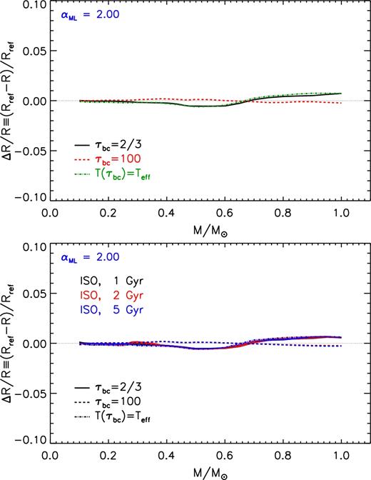
Relative radius variation as a function of the stellar mass due to the adoption of different τbc values (i.e. τbc = 2/3, 100, and T(τbc) = Teff) with respect to the reference one (τbc = 10). Top panel: models on the ZAMS. Bottom panel: models on the 1, 2, and 5 Gyr isochrones.
We performed the same analysis using the isochrones, as shown in bottom panel of Fig. 4. We found that the effect on the radius of the adopted τbc is independent of the age and it is the same shown for the ZAMS.
If αML = 1.00 is adopted, the same variations of τbc discussed above produce an effect much larger on the radius, but only for M ≳ 0.5 M⊙, as shown in Fig. 5. For τbc = 100, the effect on the radius progressively increases from about +1 per cent at 0.5 M⊙ to about +2.5 per cent at 1 M⊙. If τbc = 2/3 (or T(τbc) = Teff) is adopted, the maximum of radius change occurs between 0.4 M⊙ (−1 per cent) and 0.7 M⊙ (about −1 per cent), with a peak at about 0.6 M⊙ (about −2.5 per cent). For larger masses there is a constant variation of about −1.5 per cent. The dependence of the effect of a τbc change on the αML value is probably caused by the fact that we cannot consistently modify the αML in the atmosphere, which in all the cases, is computed for αML = 2.00. This introduces a possible discontinuity in the temperature gradient at the matching point, i.e. at τbc. However, depending on the stellar mass, if τbc is large enough the αML step change occurs in a region where the superadiabaticity is not large. In this case the αML variation (from interior to atmosphere) has a small impact, leading to a very small discontinuity in the temperature gradient. This happens, for example, when one adopts large values of τbc in VLM stars. On the other hand, if small value of τbc are used, the match between interior and atmosphere occurs where the superadiabaticity is larger, thus more sensitive to the adopted αML. In this case, the temperature gradient discontinuity can be sizeable, depending on the stellar mass, leading to an appreciable effect on the stellar structure and on its radius.
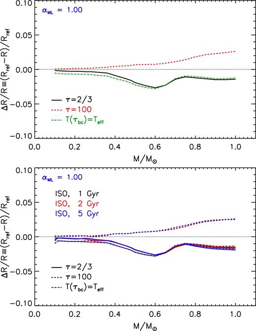
The same as in Fig. 4 but for models with αML = 1.0.
As done for the atmospheric models, we analysed the effect on the radius of adopting a solar calibrated αML in the models with perturbed τbc. Fig. 6 shows the radius variation in ZAMS induced by the quoted τbc with the corresponding solar calibrated αML, namely αML⊙ = 1.92 (τbc = 2/3), αML⊙ = 1.93 (T(τbc) = Teff), and αML⊙ = 2.05 (τbc = 100). The adoption of different values of τbc in the solar calibration does not modify the initial chemical composition but only the adopted αML. The radius variation due to the adopted τbc is progressively counterbalanced in models larger than about 0.7 M⊙ by the use of a calibrated αML⊙, as shown in figure. For lower masses, the solar calibration has no effect on the stellar radius.
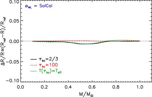
As in Fig. 4 but for solar calibrated αML values.
3.3 Radiative opacity
The uncertainty in the Rosseland radiative opacity |$\overline{\kappa }_{\rm R}$| is not provided in the opacity tables. However, it is possible to obtain an estimate of the uncertainty by comparing our reference tables (opal05) with other tables used in the literature, i.e. the OP (Badnell et al. 2005). Valle et al. (2013a, see also Tognelli et al. 2012, 2015a) showed that such a comparison suggests an average uncertainty on |$\overline{\kappa }_{\rm R}$| of about ±5 per cent in the temperature–density regime we are interested in. Such an uncertainty is approximatively the same found by Le Pennec et al. (2015) when comparing the opal and the opas (Blancard, Cossé & Faussurier 2012; Mondet et al. 2015) new set of Rosseland mean opacity tables, in solar conditions (about 6 per cent). If a wider range of temperature–pressure is considered, Mondet et al. (2015) showed that the differences between the opas and the opal tables are a bit larger reaching about 12–13 per cent, but mainly in region of low temperature and low density. We also note that recently Bailey et al. (2015) found that, in conditions similar to those at the bottom of the solar convective envelope, the predicted monochromatic iron opacity in specific wavelength ranges is drastically underestimated when compared to measured values. They also suggested that the effect of using the measured iron opacity would increase the global Rosseland mean opacity by about 4–10 per cent, at least for conditions similar to those at the bottom of solar convective envelope.
For the purpose of our investigation, we preferred to adopt an average value for the uncertainty on the radiative opacity instead of a temperature–density-dependent error. To be consistent with the uncertainty values quoted above, we adopted a rigid uncertainty of ±5 per cent in the whole temperature–density domain covered by our calculations.
The top panel of Fig. 7 shows the effect on the radius of a radiative opacity variation of ±5 per cent with respect to the reference value for the ZAMS sequence. Notice that such an opacity variation is limited to the internal region of the star, i.e. τ > τbc since the models shown in figure are computed adopting the AHF11 BCs. In this case we cannot vary the opacity in the atmosphere, since the atmospheric structure is provided as a pre-computed table.
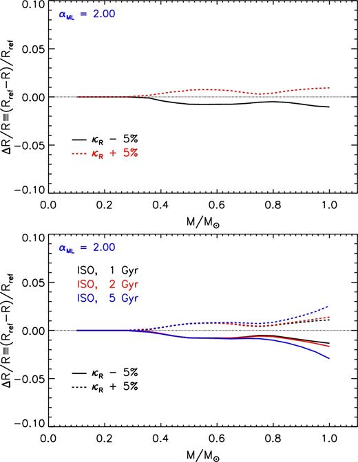
Relative radius variation as a function of the stellar mass due to the adoption of an uncertainty of ± 5 per cent on the radiative opacity coefficients (only in the stellar interior) with respect to the reference one. Top panel: models on the ZAMS. Bottom panel: models on the 1, 2, and 5 Gyr isochrones.
For M ≲ 0.3 M⊙ the opacity variation is inconsequential. This is expected as the internal structure of a star with M ≲ 0.3 M⊙ is almost adiabatic in ZAMS/MS. Under this condition the temperature gradient is mainly determined by the EOS (through the adiabatic gradient) and it is completely independent of the radiative opacity. On the other hand as the stellar mass increases, the temperature gradient in the external convective region becomes progressively more and more super adiabatic, thus more sensitive to the adopted |$\overline{\kappa }_{\rm R}$|. In addition, as the stellar mass increases above 0.4–0.5 M⊙, the ZAMS/MS model is no more fully convective, as it has developed a radiative core during the pre-MS evolution. In this cases, the opacity plays a role in determining the temperature profile also inside the internal radiative region, thus also this part of the star is sensitive to |$\overline{\kappa }_{\rm R}$| variation. The effect of varying |$\overline{\kappa }_{\rm R}$| of ±5 per cent is about 1 per cent for M ≳ 0.4 M⊙.
The bottom panel of Fig. 7 shows the effect of the opacity perturbation on the radius for models on the isochrones of 1, 2, and 5 Gyr. The relative radius variation is similar to that discussed for the ZAMS for M ≲ 0.7–0.8 M⊙, while it becomes progressively more and more sensitive to the stellar age as the mass increases. In the worst case, i.e. 5 Gyr and 1 M⊙, the perturbed radiative opacity leads to a radius variation of about 3 per cent.
The radius variation shown in Fig. 7 does not account for the opacity change in the atmosphere. Thus, to estimate the effect of an opacity variation of ±5 per cent in the whole structure, atmosphere included, we computed sets of perturbed and reference models with the KS66 BCs. In these cases, the atmospheric structure is actually computed inside our stellar code together with the interiors, allowing us to modify the opacity in the atmosphere too.3
The top panel of Fig. 8 shows the effect of an opacity variation of ±5 per cent in the whole structure when the KS66 BCs are adopted for the ZAMS sequence. For M ≲ 0.3 M⊙ the models are almost unaffected by the opacity variation even in the atmosphere, but the dependency on |$\overline{\kappa }_{\rm R}$| increases with the stellar mass. For M ≳ 0.4 M⊙ the relative differences in radius are less than 1 per cent, slightly smaller than those obtained using the non-grey BCs. Comparing the results shown in Figs 7 and 8 it emerges that the effect due to the opacity variation in the atmosphere partially counterbalances that caused by the opacity change in the interiors, thus slightly reducing the total effect on the stellar radius.
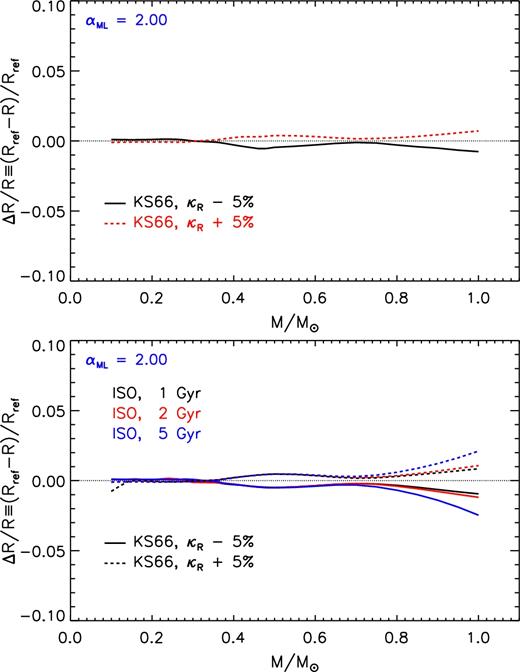
Relative radius variation as a function of the stellar mass due to the adoption of an uncertainty of ± 5 per cent on the radiative opacity coefficients in the whole structure with respect to the reference one. The perturbed and reference models have been computed adopting the KS66 atmospheric structure. Top panel: models on the ZAMS. Bottom panel: models on the 1, 2, and 5 Gyr isochrones.
The bottom panel of Fig. 8 shows the effect on the isochrones of the same opacity perturbation. The effect on the radius of the perturbed opacity depends on the age. The largest variation occurs for the 1 M⊙ model at an age of 5 Gyr, with a relative radius change of about 2–3 per cent.
Another point that deserves to be discussed is the dependence of |$\overline{\kappa }_{\rm R}$| on the adopted heavy elements abundance (i.e. elements heavier than boron). Indeed, it is well known that metals strongly contribute to the radiative opacity coefficients, especially in the external regions of a star (see e.g. Sestito et al. 2006). In the present models we assumed that the metals relative abundances are equal to those of the Sun (solar scaled mixture). However, the solar metal abundances issue is still under debate, as witnessed by the several solar abundance revisions released in recent years (e.g. Asplund, Grevesse & Sauval 2005; Caffau et al. 2008, 2011; AS09). Thus, it is worth to evaluate the effect of adopting different solar metal abundances. To do this, we compared the results obtained using the AS09 compilation (reference) and the still largely adopted Grevesse & Sauval (1998, hereafter GS98) mixture, when computing the |$\overline{\kappa }_{\rm R}$| coefficients.
Top panel of Fig. 9 shows the relative variation of the surface radius in ZAMS at a given mass if the GS98 mixture is adopted (instead of the AS09) in the |$\overline{\kappa }_{\rm R}$| coefficient computations. We used exactly the same opacity tables used for the standard models, i.e. the F05 (for low temperatures) and the opal (for high temperatures), but with the GS98 solar heavy elements abundances. The KS66 BCs have been used to check the effect of the opacity variation also in the atmosphere. The effect of the mixture on the stellar radius is almost negligible (if compared to the other uncertainty sources), being generally smaller than 1 per cent over the whole selected mass range.

Bottom panel of Fig. 9 shows the effect of the opacity variation due to the heavy element abundances on the radius for models on the isochrones. As in the previous cases, only for M ≳ 0.7 M⊙ the radius change gets sensitive to the age. The maximum effect reaches 2 per cent at 1 M⊙. We obtained similar results (for ZAMS and isochrones) using the non-grey AHF11 BCs.
For both the ZAMS and isochrones models the radius variation due to the radiative opacity change (i.e. ±5 per cent perturbation or heavy element abundance modification) is slightly dependent on the adopted αML. In particular we found that the peculiar ‘waving’ around 0.70–0.85 M⊙ tends to disappear if αML = 1.00 models are used in both ZAMS and isochrones models. The other masses are not affected by the adopted αML value.
We also checked the impact of the solar calibration on the models with the perturbed radiative opacity. A perturbation of |$\overline{\kappa }_{\rm R}$| affects not only the stellar radius but also its luminosity and temporal evolution. As a consequence, the solar calibration procedure yields values of αML⊙ and of the initial chemical composition (Y⊙ and Z⊙) different from those obtained for the reference case. In particular, by varying |$\overline{\kappa }_{\rm R}$| of +5 and −5 per cent we obtained, respectively, (Y⊙, Z⊙) = (0.2705, 0.01510) and (0.2540, 0.01537), while the initial chemical composition of the solar calibrated model in the reference case is (0.2624, 0.01523). It is evident that the radiative opacity perturbation induces a change in the initial helium (3 per cent) and metal content (1 per cent) in the Sun. On the other hand the variation of αML, due to the solar calibration, is very small, about 0.02–0.03 (KS66 BCs) or 0.03–0.04 (AHF11 BCs). Given such a situation, the change due to the different initial helium content (and metallicity) is much larger than that caused by the solar use of the calibrated αML⊙. However, keeping fixed the initial chemical composition (as discussed), we do not account for such an effect. As a consequence, the radius variation for the ZAMS or isochrones models obtained in the case of solar calibration of αML on the perturbed models is the same obtained when no calibration is performed at all, even at masses close to 1 M⊙. The same occurs if the opacity variation is caused by the adoption of a different mixture, i.e. the GS98, and the solar calibration does not change the results shown in Fig. 9.
3.4 Equation of state
As in the case of the radiative opacity, the current generation of EOS tables do not provide the uncertainties affecting the thermodynamical quantities. As such, a proper analysis of their propagation in stellar models cannot be performed. Even the simplified approach followed in the previous section for radiative opacity – by rigidly increasing/decreasing the EOS values by a constant factor – is not feasible since the different thermodynamical quantities of interest (i.e. pressure, density, adiabatic gradient, specific heat, etc.) are strictly correlated among each other. To have a first idea of the impact of the EOS uncertainty on stellar radius, we thus simply computed sets of models by changing the EOS tables, keeping fixed all the other input physics and parameters. We used two EOS largely adopted in the literature, namely the scvh95 (Saumon et al. 1995) and the FreeEOS4 (Irwin 2008). This comparison is intended to give an estimation of the agreement/disagreement level between few EOS largely used in the regime of LM and VLM stars. Note that, less recent and out-dated EOS that neglects non-ideal effects or approximatively treat partial ionizations might strongly affect the characteristics of VLM and LM stars (see e.g. Chabrier & Baraffe 1997; Siess 2001; di Criscienzo, Ventura & D’Antona 2010).
The results of the computations are shown in Fig. 10. For M ≳ 0.65 M⊙ the sole scvh95 EOS is not able to fully cover the temperature–pressure range of ZAMS models, thus the comparison is restricted on the mass range M < 0.65 M⊙.
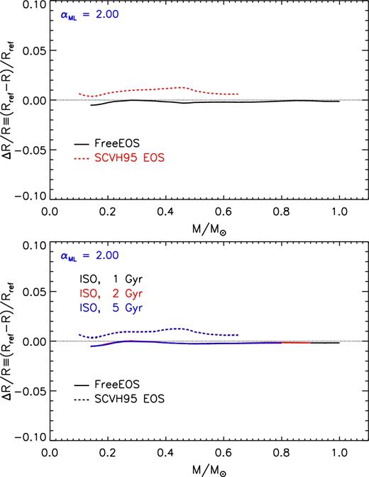
Relative radius variation as a function of the stellar mass due to the adoption of a different EOS (i.e. scvh95 and FreeEOS) with respect to the reference one (opal06+scvh95). Top panel: models on the ZAMS. Bottom panel: models on the 1, 2, and 5 Gyr isochrones.
As previously mentioned, our reference EOS is the opal extended with the scvh95 in the low-temperature–high-density regime. As such, in M ≲ 0.2 M⊙, both the EOS are used (but in different regions of the structure).
From Fig. 10 it is evident that the effect of the EOS variation on the radius is very small if the FreeEOS is adopted. This is expected as the FreeEOS has been developed to produce results similar to the opal. The largest differences between the predicted radii reaches about 1–1.5 per cent if the sole scvh95 is adopted.
It is not easy to clearly address the main cause of such differences. We checked that in the typical temperature–pressure regime of LM and VLM stars the opal06 and the FreeEOS tables provides similar values of the thermodynamical quantities of interest (i.e. CP and ∇ad), usually within ±1–2 per cent, with slightly larger values in the worst cases. On the other hand the scvh95 is sensitively different with respect to the opal. For temperatures lower than about 105 K, the relative differences of the adiabatic gradient (and specific heat) range between ±5 per cent, but they can reach, in the hydrogen and helium ionizations regions, differences up to about ±10–15 per cent.
The uncertainty due to the EOS is independent of both the stellar age (bottom panel of Fig. 10) and the αML value.
In this case we did not perform a comparison between solar calibrated αML models because (1) the sole scvh95 does not allow to compute a solar model, and (2) the FreeEOS is very similar to the opal at 1 M⊙ and the solar calibration is inconsequential.
3.5 Nuclear cross-sections
We analysed the effect of perturbing the proton–proton (pp)-chain reaction rates, namely, p(p, e+, νe)d, p(d, γ)3He, 3He(3He, 2p)4He, 3He(4He, γ)7Be, p(7Be, γ)8B, and 7Be(e−, νe)7Li, within their current uncertainty. The perturbation of the selected burning channels does not affect the radius of models in ZAMS. We also verified that it does not change the radius of models on the 1, 2, and 5 Gyr isochrones. In the following we have neglected these uncertainty sources.
3.6 Mixing length
The radius of stars with a convective envelope depends on the efficiency of the convective transport and, following the mixing length formalism, on the mixing length parameter αML. A decrease of αML translates into a less efficient energy transport – hence into a larger temperature gradient – and into a larger radius. In order to quantify such an effect in the regime of LM and VLM stars, we computed two set of models, one with the reference solar calibrated αML value (i.e. αML = 2.00) and the other with αML = 1.00. We recall that in the reference atmospheric table (AHF11) αML is fixed to 2.00 and it cannot be modified. So, we can actually analyse the impact of the adopted αML only the interior of the star. However, for VLM stars the value of αML used in the atmosphere should be not crucial, because this objects are so dense (in ZAMS) to be almost adiabatic even in the layers at the bottom of the atmosphere, which mainly determine the (Tbc, Pbc) used to derive the outer BCs (see e.g. Chabrier & Baraffe 1997; Baraffe et al. 2015). For larger masses with partially convective and superadiabatic atmosphere the situation might be different, and the effect is not quantifiable without proper atmospheric models.
Top panel of Fig. 11 shows the radius relative differences between ZAMS model computed with αML = 2.00 and 1.00. The effect of changing αML is negligible for M ≲ 0.3–0.4 M⊙, while it progressively increases up to about 14 per cent with the stellar mass. The reason of such a behaviour relies in the superadiabaticity degree inside the star. In the VLM star tail of the explored range, stars are so compact that even the convective envelope is adiabatic and hence the temperature gradient is independent of αML. On the other hand, for more massive stars the extension of the superadiabatic region in the convective envelope increases with stellar mass leading to a progressively larger sensitivity of the radius on the mixing length parameter value.
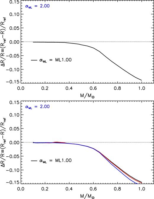
Relative radius variation as a function of the stellar mass due to the adoption of αML = 1.00 with respect to the reference one (αML = 2.00). Top panel: models on the ZAMS. Bottom panel: models on the 1, 2, and 5 Gyr isochrones.
Bottom panel shows the effect of the mixing length on the radius of models along the isochrones. There is a slight dependence on the age for the larger masses. The maximum radius variation is achieved for the 1 M⊙ at 5 Gyr (i.e. 15–16 per cent).
4 UNCERTAINTY IN THE ADOPTED INITIAL CHEMICAL COMPOSITION
To compute a stellar model, suitable initial chemical abundances have to be provided (i.e. initial helium Y, total metallicity Z, and heavy elements mixture). Unfortunately, helium abundance cannot be observed and in most of the cases only [Fe/H] is available from spectroscopy.
To estimate the effect of the initial chemical composition uncertainty on the stellar radius, we first analysed the effect of perturbing separately Y and Z, using the error in [Fe/H] and ΔY/ΔZ. To do this, first we fixed Z to its reference value (Z = 0.013) and vary ΔY/ΔZ to compute the approximated values for the perturbed Y. Secondly, we fixed Y to its reference value (Y = 0.274) and vary [Fe/H] to obtain the approximated perturbed Z values.
However, Y and Z are not independent among each other, consequently, as a second step, we analysed the effect on the total radius of simultaneously varying the couple (Y, Z) as obtained directly from equations (1) and (2) once [Fe/H], ΔY/ΔZ, and (Z/X)⊙ are perturbed within their maximum variability range.
Where not explicitly stated, we used Y = 0.274, Z = 0.013 as reference. We set the initial deuterium abundance to Xd = 2 × 10⁵ and the light elements abundances (inconsequential for this work) to the same values given in Tognelli et al. (2015a). The heavy elements abundances are obtained assuming a solar-scaled metal distribution with the AS09 abundances.
4.1 Independent variation of the initial helium abundance
The variation of the initial helium abundance Y comes essentially from the uncertainty on ΔY/ΔZ and YP. Regarding YP we used the recent value YP = 0.2485 ± 0.0008 (Cyburt 2004). Given its relatively small uncertainty, in the following, we will neglect the error of YP.
Keeping fixed the total metallicity to its reference value Z = 0.013 (and the other parameters) and perturbing only ΔY/ΔZ in equation (1), we obtained the following extreme values for Y, 0.262 and 0.287, which correspond to a variation of Y of about ±4 per cent.
Top panel of Fig. 12 shows the relative radius difference between the models with the varied initial helium abundance and the reference one for the ZAMS models. An increase of the helium content produces, at a fixed mass, a star brighter and hotter in ZAMS. The total effect is to increase the stellar radius less than 1 per cent for M ≲ 0.3–0.4 M⊙ and of about 1 per cent for larger masses. The opposite effect is achieved if the initial helium is reduced. The amount of the radius variation is symmetric because a symmetric perturbation on Y is assumed.

Relative radius variation as a function of the stellar mass due to the adoption of a different initial helium abundance (i.e. Y = 0.262 and 0.287) with respect to the reference one (Y = 0.274). Top panel: models on the ZAMS. Bottom panel: models on the 1, 2, and 5 Gyr isochrones.
Bottom panel of Fig. 12 shows the effect of the helium variation on the radius for models on the isochrones. As in the other cases, only for masses above 0.7–0.8 M⊙ the radius variation depends on the age. The maximum radius change occurs at 5 Gyr, reaching about 4 per cent.
Such differences are only marginally affected by the change of αML from 2.00 to 1.00. Only stars in the mass range 0.70–0.85 M⊙ are affected. The waving disappears and the radius variation is essentially constant to ±1 per cent. The same occurs for isochrones models.
4.2 Independent variation of the initial metallicity
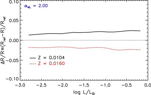
The metallicity variation δZ depends mainly on the [Fe/H] error, which we set to a conservative value of ±0.1 dex. Keeping the initial helium abundance fixed to its reference value Y = 0.274 and perturbing only [Fe/H] we obtained Z = 0.0104 and 0.0160, hence a variation of about 20 per cent with respect to the reference value.
Fig. 13 shows the total radius relative differences between models computed with the perturbed initial metallicity and the reference ones. A variation of Z affects the radiative opacity coefficients, thus producing an effect on both the interior and the atmosphere. As already discussed, depending on the stellar mass, the star reacts differently to an opacity variation in the atmosphere or in the interior. For fully convective and adiabatic ZAMS stars (M ≲ 0.4 M⊙) the variation of Z (i.e. the change of |$\overline{\kappa }_{\rm R}$|) is inconsequential in the stellar interior (τ > τbc). For such models the change of Z in the atmosphere produces a slight modification of the outer BCs that reflects in a small relative variation of the radius (less than 1 per cent). For larger masses (M ≳ 0.4 M⊙) the interior gets progressively more and more sensitive to the metallicity change through the opacity, as discussed. In this case the effect on the stellar interior dominates over the effect of δZ on the atmosphere. As a result, an increase of Z leads to a reduction of the radius (the opposite occurs if Z decreases). However, even in this case, the total effect on the radius of the metallicity is small, being of the order of about 1 per cent.
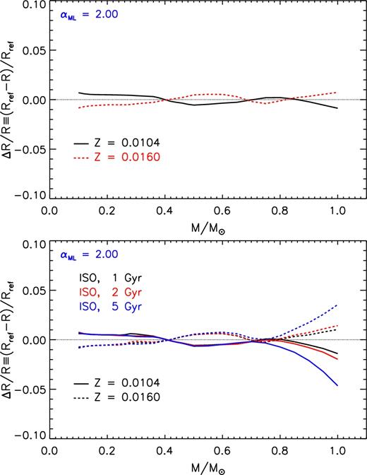
Relative radius variation as a function of the stellar mass due to the adoption of a different initial metallicity (i.e. Z = 0.0104 and 0.0160) with respect to the reference one (Z = 0.013). Top panel: models on the ZAMS. Bottom panel: models on the 1, 2, and 5 Gyr isochrones.
The effect of the initial metallicity variation on the radius depends on the age for M ≳ 0.7 M⊙. The maximum variation of the surface radius is attained by the 1 M⊙ model at 5 Gyr (i.e. about 4–5 per cent).
The radius change slightly depends on the αML in the mass range 0.70–0.85 M⊙, where the use of αML = 1.00 leads to an almost constant radius change of about 1 per cent.
4.3 Simultaneous variation of the initial helium and metallicity
As discussed in the previous section, Y and Z are correlated and the value of the couple (Y, Z) is determined by specifying the values of a triplet defined by ([Fe/H], ΔY/ΔZ, and (Z/X)⊙), as a consequence the uncertainty on these last three quantities propagates into the final uncertainty on Y and Z. In this section we discuss the variation of the stellar radius caused by the uncertainty on [Fe/H], ΔY/ΔZ, and (Z/X)⊙.
Fig. 14 shows the total radius variation for the ZAMS and isochrone models due to the uncertainty in ΔY/ΔZ. A variation of ΔY/ΔZ of ±1 affects primarily the initial helium abundance (δY/Y ∼ 4 per cent) changing the metallicity at the level of δZ/Z ∼ 1–2 per cent. As the total radius variation is mainly due to the perturbation of Y, the net effect on the models is similar to that discussed in Section 4.1.
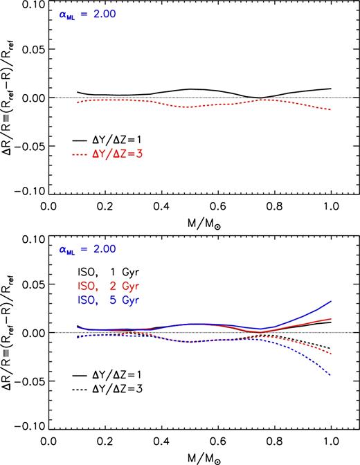
Relative radius variation as a function of the stellar mass due to the adoption of a different helium-to-metal enrichment ratio (i.e. ΔY/ΔZ = 1 and 3) with respect to the reference one (ΔY/ΔZ = 2). Top panel: models on the ZAMS. Bottom panel: models on the 1, 2, and 5 Gyr isochrones.
Top panel of Fig. 15 shows the radius relative difference between models computed with the reference and the perturbed [Fe/H] values for models along the ZAMS. A variation of [Fe/H] affects both Y and Z, but the effect on Z (about 20 per cent) is larger than that on Y (about 2 per cent). Referring to Fig. 12, a decrease of initial helium content causes a radius reduction in all the selected mass range. On the other hand the effect of Z is much complicated (Fig. 13), as for M ≲ 0.4 M⊙ the star shrinks (if Z decreases), while for larger masses it slightly increases. As a consequence of such a behaviour, the radius change due to the variation of Y almost counterbalances that caused by the metallicity perturbation for M ≳ 0.4–0.5 M⊙, while for lower values of the mass the two effects add up producing a total radius change by about ±1 per cent.
![Relative radius variation as a function of the stellar mass due to the adoption of an uncertainty of ±0.1 dex on [Fe/H] (i.e. [Fe/H] = −0.1 and +0.1) with respect to the reference one ([Fe/H] = 0). Top panel: models on the ZAMS. Bottom panel: models on the 1, 2, and 5 Gyr isochrones.](https://oup.silverchair-cdn.com/oup/backfile/Content_public/Journal/mnras/476/1/10.1093_mnras_sty195/1/m_sty195fig15.jpeg?Expires=1750500009&Signature=ruq5bW5d8vjEUbdqTEon2lujIcTLsAz6Z030vpWHHOOtwrHKdQMu9g0EScgRV-ToPgBlcPxJ59REa8bGvSBxWFsSOItufTDhw3rXoIw3y-1zotCzbUhoeLPlWOfW~IAT~KEsxWnsB2ERe2pa~IYTeVEkdvLGSadduIOyogBcJ5Vk1nAJMXXgjVvM8FcSVEhfnqXvAa7c33ucszpRluVwvDx1sS6HB1xaEZafzePhW5keJqQ6qhJR3v-e0XWAbyezp9majBlGlDnVEKY0UBq3Se9ngayMeKr4Z5dYguTQaCTZiMxUeKQNrBjODwV3VrfmR2TyDqWANrJqi7Q5~NmtNA__&Key-Pair-Id=APKAIE5G5CRDK6RD3PGA)
Relative radius variation as a function of the stellar mass due to the adoption of an uncertainty of ±0.1 dex on [Fe/H] (i.e. [Fe/H] = −0.1 and +0.1) with respect to the reference one ([Fe/H] = 0). Top panel: models on the ZAMS. Bottom panel: models on the 1, 2, and 5 Gyr isochrones.
Bottom panel of Fig. 15 shows the effect on the radius of the same variation of [Fe/H] for models on the isochrones. Only for M ≳ 0.7 M⊙ the radius variation gets progressively more and more sensitive to the stellar ages, reaching a maximum relative difference (with respect to the reference case) of about 3 per cent for 1 M⊙ at 5 Gyr.
The uncertainty on [Fe/H] produces a radius modification that is almost independent of the adopted αML. The only effect is to further flatten the radius change in the 0.70–0.85 M⊙ region leaving unchanged the variation found in the other models.
Fig. 16 shows the effect on the radius of the variation of ±15 per cent on (Z/X)⊙. We recall that the heavy elements mixture – the relative abundances of the elements heavier than boron – affects the stellar computations in two different ways: (1) through the opacity coefficients; and (2) through the total metallicity-over-hydrogen ratio (Z/X)⊙, needed to compute Z and Y (see equation 2). We already discussed the impact of the heavy element mixture on the opacity in Section 3.3, so here we limit to discuss its effect on the derived values of Y and Z.
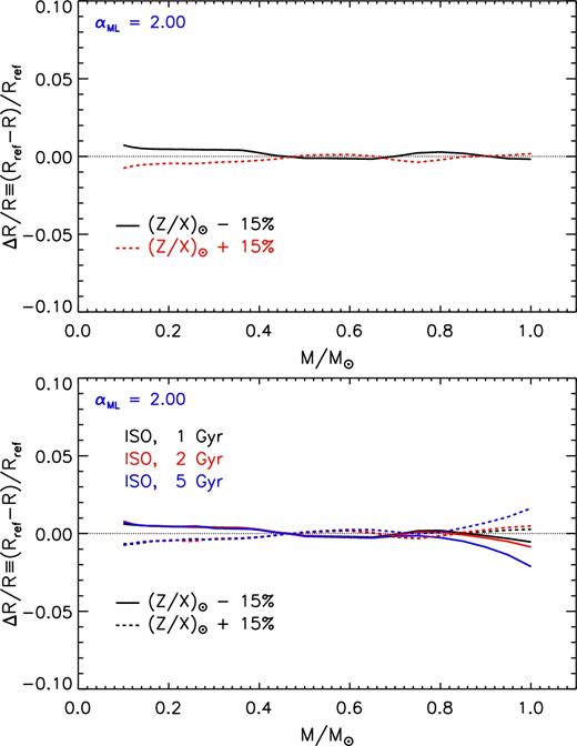
Relative radius variation as a function of the stellar mass due to the adoption of an uncertainty of ± 15 per cent on (Z/X)⊙ with respect to the reference one ((Z/X)⊙ = 0.0181; Asplund et al. 2009). Top panel: models on the ZAMS. Bottom panel: models on the 1, 2, and 5 Gyr isochrones.
An uncertainty of ±15 per cent on (Z/X)⊙ results in a variation of about 1–2 per cent in Y and about 15 per cent on Z, which is similar to that obtained by a perturbation of ±0.1 dex on [Fe/H]. Thus, the effect on the radius is essentially the same already discussed and shown in Fig. 15.
5 CUMULATIVE UNCERTAINTY
In the previous sections we quantified the individual contribution to the uncertainty of the predicted radius of each quantity, keeping fixed all the others to their reference value. Here, we evaluate the cumulative uncertainty caused by simultaneously perturbing all the investigated input physics and parameters. To do this, we started from the results obtained in previous papers, which showed that the models respond almost linearly to the perturbation/change of the quantities analysed here (Valle et al. 2013a,b; Tognelli et al. 2015a). Thus, instead of computing a huge amount of models sets where several parameters are simultaneously perturbed, we preferred to follow a more simple – but robust – approach. The edges of the variability region (i.e. the cumulative error stripe) can be obtained by linearly adding the contribution of each individual perturbation.
In the following we did not include the effect of changing αML in the total error bar, but we preferred to treat it separately from the other uncertainty sources, analysing the results for αML = 2.00 and 1.00.
The input physics and parameters that contribute to the cumulative error stripe are listed in Table 1. In many of the cases we were able to use symmetric perturbations, as in the case of the chemical composition and radiative opacity, thus obtaining upper and lower values for the radius change. In the other cases such as the EOS and BCs this was not possible, and we obtained only one edge of the error stripe. This will introduce an asymmetry in the cumulative error stripe. As for the impact of the atmospheric models on the radius we took as representative the differences between our reference (AHF11) and the BH05, neglecting both the out of date KS66 and the CK03 BCs, which is less suitable for LM stars and not available for VLM (for M ≲ 0.36 M⊙). For the evaluation of the uncertainty due to the adopted τbc we used models with τbc = 100 and 2/3.
Quantities varied in the computation of perturbed stellar models and their corresponding uncertainty/range of variation. The quantity marked with the flag ‘Yes’ has been taken into account in the calculation of the cumulative uncertainty on the stellar radius.
| Quantity | Perturbation | Cumulative |
|---|---|---|
| Input physics | ||
| τph | T(τbc) = Teff | No |
| τbc = 2/3 | Yes | |
| τbc = 100 | Yes | |
| BCs | BH05 | Yes |
| AHF11+GN93 | No | |
| CK03 | No | |
| KS66 | No | |
| |$\overline{\kappa }_\mathrm{rad}$| | ± 5 per cent | Yes |
| Solar mixture | GS98 | Yes |
| EOS | scvh95 | Yes |
| FreeEOS | Yes | |
| αML | 1.00, 2.00 | No |
| Chemical composition | ||
| [Fe/H] | ±0.1 dex | Yes |
| ΔY/ΔZ | ±1 | Yes |
| (Z/X)⊙ | ± 15 per cent | Yes |
When analysing the impact on the models of the radiative opacity uncertainty, we computed models with both non-grey AHF11 and semi-empirical KS66 BCs to take into account the opacity change in the atmosphere too. The contribution of the opacity uncertainty to the cumulative error stripe has been computed considering both cases, i.e. adding the two (quite similar) contributions to the radius change and then dividing the resulting radius variation by 2. In other words we adopted the mean value of the two sets.
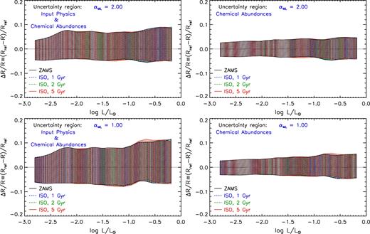
Left-hand panels of Fig. 17 show the resulting cumulative error stripe on the stellar radius that accounts for the uncertainty on both the adopted input physics and initial chemical composition in the case of ZAMS and isochrones models, for the reference mixing length parameter (i.e. αML = 2.00, upper panel, and for αML = 1.0, bottom panel).
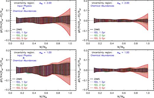
Cumulative relative radius difference for models on the ZAMS and on the 1, 2, and 5 Gyr isochrones, as a function of the stellar mass. Left-hand panels: total uncertainty due to both the errors on the adopted input physics and initial chemical composition. Right-hand panels: uncertainty due to only the errors on the initial chemical composition. Top panels: models with αML = 2.00. Bottom panels: models with αML = 1.00.
In the case of αML = 2.00, the ZAMS cumulative radius error stripe is almost symmetric, ranging from about ±2, ±3 per cent for VLM stars to about ±4, ±5 per cent at larger masses. If αML = 1.0 is used, the uncertainty on VLM and LM stars (i.e. M ≲ 0.4–0.5 M⊙) is similar to that for αML=2.00 models, while at larger masses the stripe gets progressively broader (and less symmetric), in particular for masses between 0.5 and 0.8 M⊙, where it reaches values of ±6 per cent.
Fig. 17 shows also the resulting cumulative error stripe for models on the 1, 2, and 5 Gyr isochrones, compared to the ZAMS case. The cumulative error stripe on the radius is the same of that obtained for the ZAMS for M ≲ 0.7 M⊙, while for larger masses the stripe gets progressively more and more sensitive to the chosen age, at least for ages larger than about 2 Gyr. The maximum value of the error stripe is achieved by the 1 M⊙ model at 5 Gyr, which reaches about +12(−15) per cent for αML = 2.00. The stripe for isochrones models is sensitive to the adopted mixing length parameter similarly to the ZAMS, getting broader if αML = 1.00 for M ≳ 0.5 M⊙.
We want also to clearly identify the total effect on the stellar radius due to the error on the sole initial chemical composition (i.e. helium and metal abundances). Right-hand panels of Fig. 17 show the error stripe when only the chemical composition errors are accounted for in the radius variation. The uncertainty on the initial helium and metal abundance produces a symmetric variation of the radius between ±1 and ±2 per cent for ZAMS models. The isochrone models are similar to the ZAMS for M ≲ 0.7 M⊙, while for larger masses the stripe depends on the age. In this case, the largest variation reaches about +7, −10 per cent at 5 Gyr. The uncertainty due to the chemical composition on ZAMS/isochrone models is only slightly dependent on the adopted αML (as discussed in Section 4).
The presented results showed the effect of the quoted uncertainties on the stellar radius at a fixed mass. However, it is worth to provide also the cumulative error stripe as a function of the luminosity for a direct comparison with observations when the stellar mass is not available. The perturbation of the input physics and/or chemical composition might modify both the stellar radius and the luminosity. Consequently, at the same log L/L⊙ value, the reference and the perturbed models might have different masses. Thus, in this case, the uncertainty on the stellar radius is the result of the combined variation of the radius caused by the perturbed quantity at a given mass plus the variation of the radius due to the mass change to get the same luminosity.
We verified that only in the case of perturbed outer BCs (atmospheric structures and τbc) and αML the luminosity does not change appreciably, and the radius variation at a fixed luminosity is the same of that at a fixed mass. In the other cases, the luminosity depends on the adopted value of the perturbed quantity. It might happen that the luminosity variation at a fixed mass, due to a certain perturbed quantity, shifts the radius–luminosity sequence in such a way to amplify the radius difference found at a fixed mass. This is exactly what happens, as an example, if Z is perturbed. In this case, the luminosity variation (due to the opacity enhancement/decrease) overrides the intrinsic radius change at a constant mass, producing a larger radius variation if compared to that obtained at a fixed mass. We show this effect, as a representative example, in Fig. 18. To be noted that the radius change is essentially the same in the whole luminosity range.
Relative radius variation caused by the perturbation of Z at a fixed luminosity, between the reference (Z = 0.0130) and the perturbed (Z = 0.0104 and 0.0160) ZAMS models.
Fig. 19 shows the cumulative error stripe on the radius for models on the ZAMS and on the 1, 2, and 5 Gyr isochrones as a function of the luminosity. The error stripe for ZAMS or isochrone models is essentially the same. In the case of αML = 2.00, the cumulative error stripe is asymmetric and ranges from ±4 per cent (for VLM) to about +7, +9(−5) per cent in the selected luminosity range, with the largest uncertainties occurring at higher luminosities. The stripe has a slight dependence on the adopted αML. If αML = 1.00 is considered, the cumulative error stripe ranges from +4(−6) to +8, +10(−6) per cent.
Cumulative relative radius difference between the perturbed and reference models as a function of the stellar luminosity, for models on the ZAMS and on the 1, 2, and 5 Gyr isochrones. Left-hand panels: total uncertainty due to both the errors on the adopted input physics and initial chemical composition. Right-hand panels: uncertainty due to only the errors on the initial chemical composition. Top panels: models with αML = 2.00. Bottom panels: models with αML = 1.00.
Right-hand panels of Fig. 19 show the impact of the sole chemical composition on the radius, which is between about ±3 and ±5 per cent in the whole luminosity range considered (increasing with the luminosity). Such an effect is independent of the adopted αML. Regarding the effect on the cumulative error stripe of the adoption of a solar calibrated αML⊙, we have showed in previous sections that the mixing length parameter calibration produces an effect only in the case of the BCs, reducing the radius change for M ≳ 0.7 M⊙. In all the other cases, the solar calibration is inconsequential, in particular when dealing with the chemical composition.
Fig. 20 shows the cumulative error stripe (input physics and chemical composition) for solar calibrated perturbed models as a function of the stellar mass (left-hand panel) and luminosity (right-hand panel). It is evident that the stripe is unaffected by the solar calibration for M ≤ 0.7 M⊙, while it is slightly smaller than that shown in Figs 17 and 19 for larger masses. In particular, at a fixed mass (left-hand panel of Fig. 20) for M ≳ 0.7 M⊙ the radius variation in ZAMS is almost constant to ±2, ±3 per cent, while in not solar calibrated cases it reaches 4–5 per cent. A similar behaviour can be found in the isochrone models. The effect of solar calibration is visible also at a fixed luminosity, for log L/L⊙ ≳ −1. The radius change is slightly smaller (about +6, + 7( − 4) per cent) than that obtained for not solar calibrated models (see Fig. 19). However, comparing the results found for not calibrated and calibrated αML perturbed models, we can safely conclude that the effect of the solar calibration of αML does not drastically affect the estimated error stripe.
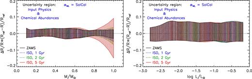
Cumulative error stripe for solar calibrated perturbed models. Left-hand panel: error stripe as a function of the stellar mass. Right-hand panel: stripe as a function of the luminosity.
6 CONCLUSIONS
We performed an analysis of the uncertainties affecting the radius predicted by stellar models of LM and VLM stars due to the errors in the adopted input physics and chemical composition.
As a first step, we analysed the impact on the radius of each input physics quantity, initial helium and metal abundance by perturbing/varying only a single quantity and fixing the other to its reference value, at a fixed mass. This method allows us to clearly address the role of each analysed quantity in determining the stellar radius variation.
Then, we computed the cumulative error stripe on the radius by adding each individual perturbation, for two different values of the superadiabatic convection efficiency, namely αML=2.0 (our solar calibrated value) and αML=1.0 first at fixed mass and then at fixed luminosity.
The cumulative error stripe at a fixed mass for ZAMS models with αML = 2.00 ranges between ±2, ±3 per cent for M = 0.1 M⊙ to about ±4, ±5 per cent at M = 1.0 M⊙. The relative error is less symmetric and broader if αML=1.0 is adopted especially for masses in the range 0.5–0.8 M⊙ reaching about ±6 per cent for M = 1.0 M⊙.
We evaluated the impact on the radius for models along the 1, 2, and 5 Gyr isochrones. For masses smaller than about 0.6–0.7 M⊙, the cumulative error stripe is essentially that given for ZAMS models, while for larger masses the radius uncertainty gets sensitive to the age, increasing with the isochrone age and reaching about +12( − 15) per cent at 5 Gyr. Similarly to the ZAMS, the cumulative stripe for the isochrones gets slightly larger if αML=1.0 is adopted.
We also showed the impact of the sole uncertainty on the adopted initial chemical composition on the radius, which is about ±1, ±2 per cent in all the selected mass range for the ZAMS, while it is larger for the isochrones, reaching +7(−10) per cent for the 5 Gyr isochrone.
We also analysed the error stripe at a fixed luminosity. In this case we found that the radius uncertainty is independent of the age and consequently the ZAMS and isochrones cumulative error stripes are coincident. The uncertainty ranges from about ±4 per cent for the faintest stars to about +7, +9(−5) per cent for the brightest stars, for αML = 2.0. The stripe gets larger if αML=1.0 is considered ranging from about +4(−6) per cent (faint stars) to +8, +10(−6) per cent (bright stars). The contribution of the sole chemical composition produces a radius variation between about ±3 and ±5 per cent in the selected luminosity range.
We also discussed the impact of a solar calibration on each of the perturbed model. We showed that only models with masses larger than about 0.7 M⊙ are actually affected by the solar calibration and that the error stripe slightly reduces in such a mass range.
ACKNOWLEDGEMENTS
We thank Gregory Feiden for his useful comments that helped to improve the paper. ET acknowledges Osservatorio Astronomico di Teramo (Modelli di accrescimento per stelle di Pre Sequenza Principale e confronto teoria-osservazione con metodi bayesiani, PI: S. Cassisi), INFN (Iniziativa specifica TAsP), and Universitá di Pisa (PRA 2016, Modellistica di stelle di piccola massa in fase di Pre-Sequenza Principale, PI: S. Degl’Innocenti).
Footnotes
The AHF11 tables are available at the URL: https://phoenix.ens-lyon.fr/Grids/BT-Settl/AGSS2009/.
A different definition/approximation of ZAMS might be adopted; however, the impact on the final results is completely negligible if compared to the variation produced by the perturbed quantities discussed in this work.
We are aware that the KS66 is not a good choice for low-mass stars, but here we are interested in a differential analysis, which is only marginally affected by the use of such atmosphere.
We used the FreeEOS in the EOS 1 configuration (as recommended by the author), which accounts for all the available ionizations states treated in detail. This configuration should give the best agreement with the opal and scvh95 EOS.
