


Abstract
Massive galaxies display extended light profiles that can reach several hundreds of kiloparsecs. We use data from the Hyper Suprime-Cam (HSC) survey that is simultaneously wide (∼100 deg2) and deep (>28.5 mag arcsec−2 in i band) to study the stellar haloes of a sample of ∼7000 massive galaxies at z ∼ 0.4. The depth of the HSC data enables us to measure surface mass density profiles to 100 kpc for individual galaxies without stacking. As in previous work, we find that more massive galaxies exhibit more extended outer profiles than smaller galaxies. When this extended light is not properly accounted for (because of shallow imaging and/or inadequate profile modelling), the derived stellar mass function can be significantly underestimated at the high-mass end. Across our sample, the ellipticity of outer light profile increases substantially with radius. We show for the first time that these ellipticity gradients steepen dramatically as a function of galaxy mass, but we detect no mass dependence in outer colour gradients. Our results support the two-phase formation scenario for massive galaxies in which outer envelopes are built up at a later time from a series of merging events. We provide surface mass density profiles in a convenient tabulated format to facilitate comparisons with predictions from numerical simulations of galaxy formation.
1 INTRODUCTION
Massive early-type galaxies (ETGs) are predicted to assemble according to a ‘two-phase’ formation scenario (e.g. Oser et al. 2010, 2012): a rapid growth phase at high redshift that is dominated by intense dissipative in situ star formation (e.g. Hopkins et al. 2008; Dekel, Sari & Ceverino 2009), and a second phase that is driven by non-dissipative processes such as dry mergers (e.g. Naab, Khochfar & Burkert 2006; Khochfar & Silk 2006), with an important role played by minor mergers (e.g. Hilz et al. 2012; Hilz, Naab & Ostriker 2013; Oogi & Habe 2013; Bédorf & Portegies Zwart 2013; Laporte et al. 2013). Both numerical simulations (e.g. Oser et al. 2010) and semi-analytic models (SAM; e.g. Lee & Yi 2013, 2017) agree that the fraction of stellar mass accreted in the second phase (the ex situ component) should increase with total galaxy stellar mass (e.g. Lackner et al. 2012; Cooper et al. 2013; Qu et al. 2017). For instance, recent results from the Illustris1 simulation (Vogelsberger et al. 2014, Genel et al. 2014) predict that the fraction of accreted stars increases significantly with galaxy mass, reaching faccreted > 0.5 at log (M⋆/M⊙) >11.5 (Rodriguez-Gomez et al. 2016).2
Given the success of the ‘two-phase’ scenario in explaining the properties of high-z massive quiescent galaxies (e.g. van Dokkum et al. 2010; van der Wel et al. 2011; van de Sande et al. 2011; Belli, Newman & Ellis 2014) and the dramatic increase of their effective radii (Re; e.g. Newman et al. 2012; van der Wel et al. 2014), it is time to confront this model with additional observations, in particular, the detailed surface mass density profiles of low-redshift massive galaxies. Early studies based on 1D light profiles found that the surface mass density profiles of nearby ETGs are well described by single-Sérsic profiles (e.g. Kormendy et al. 2009; except for the most central regions) and that the Sérsic index increases with total luminosity (e.g. Graham 2013). A more recent study of the surface brightness profiles of ETGs revealed that ETGs belong to two families: those that follow single-Sérsic law, versus those that significantly deviate from the single-Sérsic profile (Schombert 2015). 2D analyses have also found that the stellar distributions of massive ETGs are often better described by multiple-component models (e.g. Huang et al. 2013a; Oh, Greene & Lackner 2017). Huang et al. (2013b), further suggesting a connection between the multicomponent nature of massive galaxies and their two-phase assembly histories.
To further confront the two-phase scenario requires very deep observations of large samples of massive ETGs to correctly estimate their total stellar masses (e.g. Bernardi et al. 2013; D'Souza et al. 2014), as well as to quantify the amplitude and scatter among outer envelopes (e.g. Capaccioli et al. 2015; Iodice et al. 2016, 2017). To date, large samples of massive galaxies with deep imaging have been lacking. Even in the nearby universe, it is not trivial to map the low surface brightness outskirts of massive galaxies (e.g. Capaccioli et al. 2015; Iodice et al. 2016, 2017; Spavone et al. 2017; Mihos et al. 2017). Some of these measurements are based on image stacking methods (e.g. Tal & van Dokkum 2011; D'Souza, Vegetti & Kauffmann 2015). The number of very massive galaxies is also very limited in the local universe. For example, according to the MASSIVE survey (Ma et al. 2014), there are only ∼60–70 massive galaxies with log (M⋆/M⊙)>11.6 (based on K-band luminosity) within 108 Mpc.
In addition to mass density profiles, the radial profile of ellipticity also contains information about the 3D geometry (e.g. Tremblay & Merritt 1995, 1996; Chang et al. 2013; Rodríguez & Padilla 2013; Mitsuda et al. 2017) and kinematics (e.g. Cappellari et al. 2012; Weijmans et al. 2014) of stars in massive galaxies. If the stellar haloes of massive galaxies are indeed dominated by accreted stars, their ellipticities could be systematically different with the inner regions and may contain clues about the assembly history of massive galaxies (e.g. average time since last merger and average merger mass ratio). These issues have not been fully explored in both simulation and observation. Certain simulation predicts that a more massive ETG should have rounder shape (e.g. Wu et al. 2014), while others generate massive galaxies with very elongated haloes (e.g. Li et al. 2017). On the observational side, constraints are only available from a few works that use either an image stacking method (e.g. Tal & van Dokkum 2011; D'Souza et al. 2015) or a small sample of nearby galaxies (e.g. Spavone et al. 2017).
In this paper, we take advantage of the high-quality deep images from the Hyper Suprime-Cam (HSC) Subaru Strategic Program (SSP, Aihara et al. 2017a, see Section 2.1 for details) to characterize the light profiles of massive galaxies out to 100 kpc. We select a large sample (∼7000) of massive central galaxies at 0.3 < z < 0.5 using ∼100 deg2 of data from the HSC wide layer.
We use this sample to (1) reliably estimate individual surface mass density (μ⋆) profiles of massive galaxies out to 100 kpc, (2) investigate the dependence of their outer stellar haloes on total stellar mass and (3) examine the implications in terms of evaluating the high-mass end of the galaxy stellar mass function (SMF). In the second paper in this series (Huang et al. in preparation), we will investigate the environmental (dark matter halo mass) dependence of the sizes of massive ETGs (Huang et al. in preparation) .
This paper is organized as follows. Section 2 presents our data and initial sample selection. Section 3 describes our procedure for extracting 1D surface brightness profiles. Section 4 describes how we estimate stellar mass. Section 5 summarizes the final sample selection procedure. Our main results are presented in Section 6 and discussed in Section 7. Section 8 presents our summary and conclusions.
Magnitudes use the AB system (Oke & Gunn 1983), and are corrected for galactic extinction using calibrations from Schlafly & Finkbeiner (2011). In this work, we assume H0 = 70 km s−1 Mpc−1, Ωm = 0.3, and ΩΛ = 0.7. Stellar mass is denoted M⋆ and has been derived using a Chabrier initial mass function (IMF; Chabrier 2003). Halo mass is defined as |$M_{\rm 200b}\equiv M(<r_{\rm 200b})=200\bar{\rho } \frac{4}{3}\pi r_{\rm 200b}^3$| where r200b is the radius at which the mean interior density is equal to 200 times the mean matter density (|$\bar{\rho }$|).
We emphasize that in this work we do not attempt to disentangle the galaxy light from any ‘intracluster’ light component (ICL; e.g. Carlberg, Yee & Ellingson 1997; Lin & Mohr 2004; Gonzalez, Zabludoff & Zaritsky 2005; Mihos et al. 2005). Although the rising stellar velocity dispersion in the outskirts of massive brightest cluster galaxy (BCG) hints at a kinematically separated ICL component (e.g. Dressler 1979; Carter, Bridges & Hau 1999; Kelson et al. 2002; Bender et al. 2015; Longobardi et al. 2015), it is extremely difficult to reliably isolate it photometrically. Moreover, both the stellar halo of the main galaxy and the ICL component carry important information regarding the assembly history of the central galaxy and its dark matter halo. Therefore, we adopt the view that the light of the main galaxy and the ICL component trace different scales of a single, smooth, and continuous distribution.
2 DATA AND SAMPLE SELECTION
2.1 The Hyper Suprime-Cam Survey
The SSP (Aihara et al. 2017b, 2017a) makes use of the new prime-focus camera, the HSC (Miyazaki et al. 2012, Miyazaki in preparation), on the 8.2-m Subaru telescope at Mauna Kea. The ambitious multilayer HSC survey takes advantage of the large field of view (1|$_{.}^{\circ}$|5 in diameter) of this camera and will cover >1000 deg2 of sky in five broad-bands (grizy) to a limiting depth of r ∼ 26 mag in the WIDE layer. This work is based on the internal data release (DR) S15B, which covers ∼110 deg2 in all five bands to full WIDE depth. The regions covered by this release overlap with a number of spectroscopic surveys [e.g. Sloan Digital Sky Survey (SDSS)/Baryon Oscillation Spectroscopic Survey (BOSS): Eisenstein et al. 2011, Alam et al. 2015; Galaxy And Mass Assembly (GAMA): Driver et al. 2011, Liske et al. 2015. S15B release has similar sky coverage with the Public DR 1 (Please see table 3 in Aihara et al. 2017a for detailed comparison).
The HSC WIDE survey is about 3.0–4.0 mag deeper in terms of the i-band surface brightness limit than SDSS. Combined with the excellent imaging resolution (the median i band seeing is 0.6 arcsec ) and the wide area, the HSC survey represents an ideal data set to perform statistical studies of the surface brightness profiles of massive galaxies out to their distant outskirts. Fig. 1 illustrates the quality of HSC imaging compared to SDSS for three low-redshift ETGs, and shows that HSC survey data are well suited for mapping the stellar distribution of massive galaxies out to large radii.
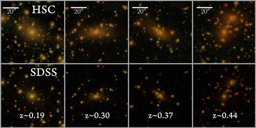
A comparison between the depth and imaging quality of SDSS and the HSC wide layer for a sample of nearby massive elliptical galaxies at 0.2 < z < 0.5. These images are generated using gri-band images with an arcsinh stretch (Lupton et al. 2004). The HSC WIDE layer is 3.0–4.0 mag deeper than SDSS.
HSC i-band images typically have the best seeing compared to other bands because of strict requirements driven by weak-lensing science. We therefore use i-band images to measure the stellar distributions of massive galaxies.
2.2 HSC data processing
The full details of the HSC data processing can be found in Bosch et al. (2017) and are briefly summarized here. The HSC SSP data are processed with hscPipe 4.0.2, a derivative of the Large Synoptic Survey Telescope (LSST) pipeline (e.g. Jurić et al. 2015; Axelrod et al. 2010), modified for HSC. hscPipe first performs a number of tasks at the single exposure level (bias subtraction, flat fielding, background modelling, object detection, and measurements). Astrometric and photometric calibrations are performed at the single exposure level. hscPipe then warps different exposures on to a common World Coordinate System and combines them into co-added images. At this stage, hscPipe updates the images with a better astrometric and photometric calibrations using stars that are common among exposures.
The pixel scale of the combined images is 0.168 arcsec. Photometric calibration is based on data from the Panoramic Survey Telescope and Rapid Response System (Pan-STARRS) 1 imaging survey (Schlafly et al. 2012, Tonry et al. 2012, Magnier et al. 2013). To achieve consistent deblending and photometry across all bands, hscPipe performs multiband post-processing at the coadd level. First, hscPipe performs object detection on coadd images in each band independently and records the flux peak and the above-threshold region (referred as a footprint) for each source. Next, footprints and peaks from different bands are merged before performing deblending and measurements. Finally, hscPipe selects a reference band for each object based on the signal-to-noise ratio (S/N) in different bands. (For most galaxies in this work, the reference band is the i band.) After fixing the centroids, shape, and other non-amplitude parameters of each object in this reference catalogue, hscPipe performs forced photometry on the coadd image in each band. This forced photometry approach is optimized to yield accurate galaxy colours at iCModel ≤ 25.0 mag (see Huang et al. 2017).
For each galaxy, hscPipe measures a cModel magnitude using an approach that is similar to SDSS (Bosch et al. 2017). However, as opposed to SDSS, the HSC cModel is based on forced multiband photometry, which means that it can accurately measure both the fluxes and colours of galaxies. The HSC cModel algorithm fits the flux distribution of each object using a combination of a de Vaucouleur and an exponential component and accounts for the point spread function (PSF). The performance of this algorithm has been tested using synthetic objects (Huang et al. 2017), and the results indicate that, generally speaking, the HSC cModel photometry is accurate down to i > 25.0 mag. However, cModel currently systematically underestimates the total fluxes of massive ETGs with extended stellar distributions. This is caused by an intrinsic limitation of cModel, as it is incapable of modelling profiles with extremely extended outskirts, a problem that is exacerbated at the depth of the HSC survey. In addition, at the depth of the HSC survey, it is challenging to accurately deblend in the vicinity of large ETGs, where satellites and background galaxies often blend with the low surface brightness stellar envelope. The deblending method currently implemented in hscPipe tends to ‘overdeblend’ the outskirts of bright galaxies and leads to an underestimation of the total flux of massive ETGs. (This is discussed further in Bosch et al. 2017.) For these reasons, our results are based on custom-developed code to measure the luminosities and stellar masses of massive galaxies. We use the HSC hscPipe photometry for two purposes: (1) to perform a first broad sample selection, and (2) to estimate the average colour of massive galaxies.
2.3 Initial massive galaxy sample
We begin by using a broad flux cut to select an initial sample of massive galaxies at z < 0.5 from the HSC photometric catalogue. Based on Leauthaud et al. (2016), iSDSS, cModel ≤ 21.0 mag can define a sample that includes almost all log (M⋆/M⊙)≥11.5 galaxies. We therefore perform an initial conservative selection of massive galaxies with iHSC, cModel ≤ 21.5.3 We also limit our sample to regions that have reached the required depth of the WIDE survey in i band as defined in Aihara et al. (2017a).
We further select extended objects with no deblending errors, with well-defined centroids, and with useful cModel magnitudes in all five bands. After removing objects that have pixels affected by saturation, cosmic rays, or other optical artefacts,4 this sample corresponds to 1760 845 galaxies and is referred to as hscPho.
Here, we limit our study to the very high-mass end where the majority of galaxies have either a spectroscopic redshift or a robust red-sequence photo-z from the redMaPPer galaxy cluster catalogue5 (e.g. Rykoff et al. 2014; Rozo et al. 2015).
We match the hscPho sample with a spec-z catalogue compiled by the HSC team. The catalogue is created by matching HSC objects with a series of publicly available spectroscopic redshifts (e.g. SDSS DR 12, Alam et al. 2015; GAMA DR2, Liske et al. 2015). The spec-z quality flags from different catalogues are homogenized into a single flag that indicates secure redshifts. Please see section 4.4.2 of Aihara et al. (2017a) for details of this catalogue. To ensure reasonable M⋆ completeness at the high-M⋆ end, we focus on the redshift range 0.3 ≤ z ≤ 0.5.
Objects without a spectroscopic redshift are matched with central galaxies from the redMaPPer SDSS DR8 (Rykoff et al. 2014) catalogue using a 2.0 arcsec matching radius. Matched objects with a red-sequence photo-z (0.3 ≤ zλ < 0.5) are included in our sample. The accuracy of the red-sequence photo-z is sufficient (median |zλ − zSpec| ∼ 0.01) for our purpose. The redMaPPer catalogue provides an additional 133 unique redshifts for massive galaxies in our sample.
In total, at 0.3 ≤ z ≤ 0.5, our sample consists of 25 286 galaxies with reliable redshift information (referred as hscZ).
The majority of our redshifts comes from the BOSS and SDSS ‘legacy’ luminous red galaxy (LRG) samples. The GAMA survey provides an additional 14 per cent of all spectroscopic redshifts. Although the GAMA survey only covers parts of the S15B DR, and hence affects the homogeneity of our sample, it does not affect the results of this work. We discuss this more in Section 5.
We choose the redshift range 0.3 ≤ z ≤ 0.5 to make sure that (1) the inner region of massive galaxies can be resolved, and M⋆ within 10 kpc can be reliably measured; (2) the background noise and cosmological dimming are not major issues so that the μ⋆ profile can be measured out to >100 kpc; and (3) redshift evolution in the stellar population properties can be largely ignored. Also, at higher redshift, the completeness of the spec-z sample starts to decline; at lower redshifts, the oversubtraction of the background level becomes a more serious issue.
We now describe our 1D photometric analysis (Section 3) and our stellar mass estimates (Section 4). We define the final sample in Section 5.
3 MEASUREMENTS OF 1D SURFACE BRIGHTNESS PROFILES
The surface brightness profiles of massive ETG are not well modelled by the de Vaucouleurs or single-Sérsic law, especially at the imaging depth of HSC. These models fail to simultaneously describe the profile in both the inner and the outer regions and also cannot account for any radial variations in ellipticity and position angle. Although they can still be described by more complex models (e.g. Huang et al. 2013a,b; Oh et al. 2017), the results are sensitive to the choice of model, the number of components, and internal degeneracies among parameters. 2D modelling is also very sensitive to background subtraction method, especially for massive ETGs (e.g. Huang et al. 2013a).
We therefore perform elliptical isophote fitting using the Image Reduction and Analysis Facility (iraf) Ellipse algorithm (Jedrzejewski 1987) to estimate the total luminosities of massive galaxies and to measure their 1D stellar mass surface density profiles (μ⋆) . This 1D method is less affected by the issues mentioned above. Also, we only study galaxies in the radial range where our results are less sensitive to either the PSF or the background subtraction. We ignore the inner ∼6 kpc, which is twice the size of 1 arcsec seeing at z = 0.5. Using this conservative choice, we can safely ignore the smearing effect of seeing outside this radius. As we discuss below, we confirm this by comparing our HSC profiles with observations with higher spatial resolution. As for the impact from background subtraction, we focus on the profiles within 100 kpc. This is an empirical but also conservative choice based on the tests, we conducted on background-corrected postage stamps. Once the surrounding objects are appropriately masked out, the extracted 1D surface brightness profiles rarely see unphysical truncation or fluctuation within 100 kpc, especially for the log (M⋆, 100kpc/M⊙)>11.6 galaxies. Please see Appendix B for more details on these tests.
We generate a postage stamp of each galaxy that extends to 750 kpc in radius, along with the bad pixel mask and the PSF model. The postage stamps are large enough to evaluate the local background. We choose to use i-band images since they trace the stellar mass distributions of 0.3 ≤ z ≤ 0.5 massive galaxies reasonably well (corresponds to rest-frame g or r band). i-band images also enable better seeing and lower background levels than the z- and y-band images, although these bands are better tracers of μ⋆.
To overcome the hscPipe ‘overdeblending’ issue, we use a customized procedure on each postage stamp to detect and aggressively mask out neighbouring objects. Furthermore, hscPipe tends to oversubtract the background around bright objects. To improve the background subtraction, we first aggressively mask out all objects (including the central massive galaxy), and derive an empirical background correction using SExtractor. These procedures are described in detail in Appendix B. We should point out that we do not use the photometric results from our customized process, but simply rely on them for improved local background model and appropriate object mask.
Then, we run Ellipse on the background-corrected, masked postage stamp following the methodology of Li et al. (2011). In short, we first fit each isophote using a free centroid and shape (ellipticity and position angle). We then fix the centroid (using the mean flux-weighted centroid) and estimate the mean ellipticity and position angles of all isophotes. Finally, we extract a 1D surface brightness profile along the major axis using the mean ellipticity and position angle. We correct these profiles for galactic extinction and cosmological dimming, and we integrate them to various radii to get the luminosity within different physical (elliptical) apertures. Fig. 2 shows an example of the 1D surface brightness and ellipticity profile for a massive galaxy at z ∼ 0.2 and also highlights a few isophotes.
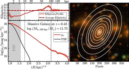
Left: example of the 1D surface brightness and ellipticity profile of a massive galaxy at z = 0.23 in the i band extracted using Ellipse. In this work, we always show the radial profile using an R1/4 scaling on the x-axis. By using this scale, the de Vaucouleurs profile will appear as a straight line on this figure. We also plot the relative brightness profile of the PSF model normalized at the central surface brightness of the galaxy to highlight the region most strongly affected by seeing. The grey shading highlights the region (r < 6 kpc) that is equivalent to twice the size of the half-width of a 1 arcsec seeing at z ∼ 0.5. Because it is a very conservative estimate of the region, we cannot reliably extract a 1D profile due to the smearing effect of seeing. On the top panel, the dashed line shows the mean ellipticity used for the final isophote. Right: the three-colour image of this galaxy with isophotes extracted by Ellipse. The thick dotted line highlights the isophote with μi ∼ 28.5 mag arcsec−2.
We test our procedure using different mask sizes and different Ellipse parameters; we also test the procedure with and without our background correction. Based on these tests, we find that our 1D surface brightness profiles are reliable up to surface brightness levels of i ∼ 28.5 mag arcsec−2. Beyond that, some of our profiles show signs of truncation and/or large fluctuations, which are due to either the uncertainty in the background subtraction or the unmasked flux from other objects. We choose to limit our study to surface brightness levels up to ∼28.5 mag arcsec−2. This is a conservative choice, but is sufficient to enable us to measure light profiles out to 100 kpc on a galaxy-by-galaxy basis (no stacking). The 1D method fails to extract profiles for ∼10 per cent of the sample due to severe contamination of other objects; these profiles are excluded from the analysis. For additional technical details on the Ellipse procedure, please see Appendix B.
4 STELLAR MASSES AND MASS DENSITY PROFILES
4.1 Stellar masses from SED fitting
To convert luminosities into M⋆, we assume that these massive galaxies can be well described by an average M⋆/L. This is a reasonable assumption considering that they are mostly dominated by old stellar populations and are known to have only shallow colour gradients (e.g. Carollo, Danziger & Buson 1993; Davies, Sadler & Peletier 1993; La Barbera et al. 2012; D'Souza et al. 2014). We discuss more about this point in Appendix C, and our own measurements of colour profiles (see Section 6.3) also demonstrate this point.
We use the broad-band spectral energy distribution (SEDs) fitting (see Walcher et al. 2011 for a recent review) code iSEDFit6 (Moustakas et al. 2013) to estimate the average M⋆/L and k-corrections using five-band HSC cModel fluxes. iSEDFit uses a simplified Bayesian approach to estimate the posterior probability distribution functions (PDF) of key stellar population parameters. Although cModel tends to underestimate the total fluxes of bright, extended objects, it can still yield accurate average colours thanks to the forced-photometry method that takes the PSF convolution into account (e.g. Huang et al. 2017).
Here, we estimate average M⋆/L using the Flexible Stellar Population Synthesis7 (FSPS; v2.4; Conroy & Gunn 2010a, Conroy & Gunn 2010b) model based on the Medium-resolution Isaac Newton Telescope Library of empirical Spectra (MILES)8 (Sánchez-Blázquez et al. 2006, Falcón-Barroso et al. 2011) stellar library, with a Chabrier (2003) IMF between 0.1 and 100 M⊙and metallicity ([M/H] = log(Z/Z⊙)) between 0.004 and 0.03. We assume a delayed-τ model with stochastic star bursts for the star formation history (SFH; see Appendix C) of low-z massive galaxies (e.g. Kauffmann et al. 2003). The Calzetti et al. (2000) extinction law is adopted in this work. The massive ETGs in our sample are not very sensitive to the SFH shape or the internal dust extinction.
We construct five-band SEDs using the forced-photometry cModel magnitudes corrected for Galactic extinction. Presently, cModel only accounts for the statistical error on the flux measurement and it certainly underestimates the true flux errors of bright galaxies. For this work, we supply iSEDFit with simplified flux errors assuming S/N = 100 for the riz bands, and S/N = 80 for the g and y band (on average, images in gy bands are shallower in depth and/or have higher background noise). These empirical S/N choices still only provide lower limits of the true systematic uncertainties from the model-fitting process. In Huang et al. (2017), we evaluate the accuracy of HSC cModel photometry using synthetic galaxies, and show that cModel provides excellent measurements of five-band colours, which are crucial for reliable M⋆/L estimates. The typical uncertainty of log (M⋆/M⊙) is around 0.06–0.08 dex at log (M⋆/M⊙)∼11.5.
In Appendix C, we briefly summarize the basic statistics of the sample by showing the relationships between M⋆, 100kpc and stellar age, metallicity, and internal dust extinction. All these properties behave reasonably for massive galaxies in this sample. Using the k-corrected optical colour, we can also confirm that the sample follows a tight ‘red sequence’.
4.2 Definitions of different aperture stellar masses
iSEDFit helps us estimate the best-fitting M⋆ based on the cModel photometry (noted as M⋆, cModel) and the average M⋆/L in the i band. Then, we can convert the 1D luminosity density profiles into stellar mass surface density (μ⋆) profiles with the average M⋆/L and estimate M⋆ within different radius by integrating the μ⋆ profiles. Given exquisite μ⋆ profiles extending to >100 kpc, the definition and meaning of ‘total’ M⋆ becomes nuanced. At the same time, motivated by the two-phase scenario, M⋆ within different radius may help us trace different physical components. Considering this, here we define a few benchmark physical apertures throughout this work:
The M⋆ within the inner 10 kpc (hereafter noted M⋆, 10kpc). Suggested by recent observation (e.g. van Dokkum et al. 2010) and simulation (e.g. Rodriguez-Gomez et al. 2016), the in situ component dominates the M⋆ within one effective radius (Re, or 5–10 kpc) of z ∼ 0 massive ETGs. We therefore use M⋆, 10kpc as the M⋆ of the inner ‘core’ and as a proxy for the in situ M⋆. The high-quality HSC data enable us to reliably measure M⋆, 10kpc at 0.3 < z < 0.5 (1.0 arcsec in radii equal 4.4 and 6.1 kpc at redshifts 0.3 and 0.5, respectively). We should point out that in simulation an (e.g. Rodriguez-Gomez et al. 2016), in situ component can extend outside the inner 10 kpc, while an ex situ component may contribute to M⋆, 10kpc at the same time. We further discuss this assumption in Section 7.1.
The M⋆ within 100 kpc (hereafter noted M⋆, 100kpc). For massive galaxies in our sample, 100 kpc aperture corresponds to 5–10 × Re and should contain the majority of the M⋆. Here, we use M⋆, 100kpc as a measure of the ‘total’ M⋆. We show that, although not perfect, M⋆, 100kpc is a better tracer of total M⋆ than model-dependent results from shallower images that rely on extrapolating the light profiles out to large radii. We should point out that the S/N for surface brightness measurement at S/N is still above the limit set by the intrinsic fluctuation of the background for our massive galaxies (e.g. see Pohlen & Trujillo 2006).
The M⋆ within the largest available aperture (hereafter noted M⋆, Max). We know that the μ⋆ profiles of massive galaxies extend way beyond 100 kpc with no clear sign of truncation (e.g. Gonzalez et al. 2005; Tal & van Dokkum 2011; D'Souza et al. 2014). Therefore, M⋆, 100kpc should be only considered as the lower limit of the ‘total’ M⋆. Here, we also integrate the μ⋆ profile to the edge of the postage stamp, and we select the isophote that gives us the highest M⋆ and define the M⋆, Max. These procedures help us quantify how much extra M⋆ may be kept at >100 kpc.
All aperture M⋆ are measured after adopting an isophote with fixed ellipticity and position angle, and instances of 10ss and 100 kpc refer to the radius along the major axis of the elliptical isophote.
In Fig. 3, we compare the different definitions of M⋆. As expected, directly measured light out to 100 kpc helps us recover more M⋆ compared to M⋆, cModel. At high-M⋆ end (e.g. log (M⋆, 100kpc/M⊙)>11.6), the average difference is larger than 0.1 dex and can be as large as 0.2–0.3 dex. For the cModel photometry in the current hscPipe, the average difference relates to both the intrinsic limitations cModel algorithm and the oversubtracted background. In Section 6.2, we use the μ⋆ profiles to show that a large fraction of these galaxies have μ⋆ profiles shallower than the de Vaucouleurs profile; it is therefore not surprising that cModel systematically underestimates the luminosity. More importantly, the differences clearly depend on total stellar mass, as M⋆, cModel tends to miss more M⋆ in more massive galaxies. This limitation in M⋆, cModel relates to the mass-dependent nature of the stellar haloes of massive galaxies (see Section 6.2 too). These differences have important implications for estimates of the SMF and for studies of the environment dependence of galaxy structure.
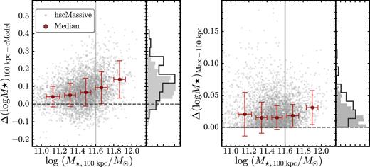
Left:difference between M⋆, cModel and M⋆, 100kpc for massive galaxies (grey dots). The running median of the mass difference is shown by large red hexagons. On average, M⋆, cModel underestimates the total stellar mass of massive galaxies by 0.1 dex, while in some cases, the difference can exceed 0.2 dex. Vertical histograms indicate the mass difference for all galaxies (shaded histogram) and for the ones with log (M⋆, 100kpc/M⊙)>11.6 (empty histogram). Right: difference between M⋆, Max and M⋆, 100kpc in the same format. The average difference is small (0.02 dex) and has no clear mass dependence. Please note that the scales of the vertical axes are different for these two figures.
The right-hand panel of Fig. 3 compares M⋆, Max and M⋆, 100kpc. Uncertainties in the background subtraction and the impact of neighbouring objects make M⋆, Max more uncertain than M⋆, 100kpc. None the less, we still see that M⋆, Max becomes larger than M⋆, 100kpc. The differences are on average very small (∼0.02–0.03 dex) and do not show strong mass dependence. This confirms that, at the current depth of HSC images, M⋆, 100kpc can be used as a good proxy of ‘total’ stellar mass.
4.3 Stellar mass completeness
With the help of the Stripe82 Massive Galaxy Catalogue (S82-MGC, Bundy et al. 2015),9 we investigate the M⋆ completeness of our samples. The S82-MGC sample matches the deeper SDSS photometric data in the Stripe 82 region (Annis et al. 2014) with the near-infrared data from the United Kingdom Infrared Telescope Infrared Deep Sky Survey (UKIDSS; Lawrence et al. 2007), and is complete to log (M⋆/M⊙)≥11.2 at z < 0.7, which makes it sufficient to evaluate the completeness of our HSC sample. Leauthaud et al. (2016) use this sample to show that the BOSS spec-z sample, which is our main source of redshifts, is about 80 per cent complete at log (M⋆/M⊙)≥11.6 at 0.3 < z < 0.5.
Fig. 4 compares the number density distributions of galaxies from S82-MGC with the 20 453 galaxies that are also in our sample.10 To be consistent with the S82-MGC catalogue, we estimate the M⋆, cModel of these galaxies using iSEDFit. We find excellent agreement between HSC M⋆, cModel and the ones from the S82-MGC catalogue.
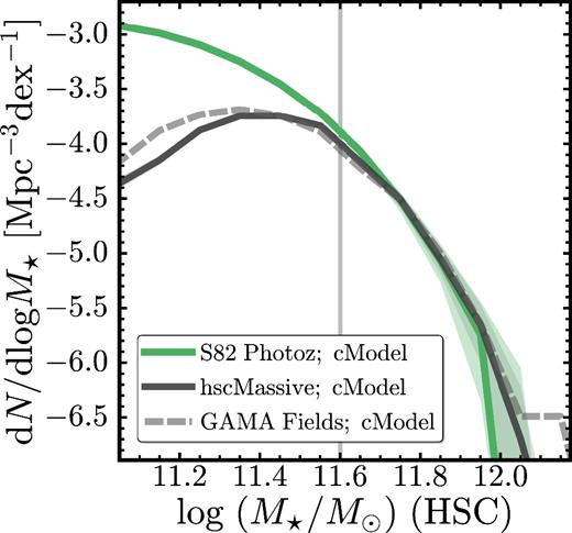
Evaluation of the M⋆ completeness of the HSC massive galaxy sample. We compare the volume number density function of the massive galaxies for this work (black line) with the one of a much more complete sample from the S82-MGC catalogue (green line). The grey dashed line shows the number density function of HSC massive galaxies in the three GAMA fields for comparison. The associated uncertainties derived from bootstrap resampling are shown in shaded regions. The vertical grey line highlights the log (M⋆/M⊙)=11.6 limit. Below the limit, the HSC massive galaxy sample becomes significantly incomplete in stellar mass.
We conclude that our sample of massive galaxies is reasonably complete down to log (M⋆, cModel/M⊙)∼11.5 at 0.3 ≤ z ≤ 0.5. Given the average difference between M⋆, 100kpc and M⋆, cModel, we chose to focus on galaxies with log (M⋆, 100kpc/M⊙)>11.6. In Section 7, we also show results for massive galaxies with 11.4 ≤log (M⋆, 100kpc/M⊙)<11.6, but we caution that our sample is incomplete in this lower mass bin mainly due to the intrinsic incompleteness of the SDSS/BOSS spec-z (see Leauthaud et al. 2016).
5 THE FINAL SAMPLE
5.1 Candidate massive central galaxies
Typically, a ‘central’ galaxy is defined as a galaxy located in the centre of its own dark matter halo, while a galaxy in a sub-halo orbiting within the virial radius of a more massive halo is referred to as a ‘satellite’ (e.g.Yang et al. 2007). We wish to focus on massive central galaxies here as they are essential to the study of galaxy–halo connection. Although the satellite fraction is expected to be very low (<10 per cent; e.g. Reid et al. 2014; Hoshino et al. 2015; Saito et al. 2016) at log (M⋆, 100kpc/M⊙)>11.6, we further use the redMaPPer cluster catalogue (v5.10; e.g. Rykoff et al. 2014; Rozo et al. 2015) based on SDSS DR8 (Aihara et al. 2011) to help us identify centrals of cluster-level dark matter haloes and reduce satellite contamination.
After matching the hscZ sample with the central galaxies of redMaPPer clusters with richness λ ≥ 2011 and central probability PCen ≥ 0.7, we find 164 matched galaxies at 0.3 ≤ z ≤ 0.5. According to available calibration (e.g. Saro et al. 2015; Farahi et al. 2016; Melchior et al. 2016; Simet et al. 2017), they represent the central galaxies in dark matter haloes with log (M200b/M⊙)<14.0; we refer to these galaxies as the cenHighMh sample .
As the next step, we identify and remove all galaxies within a cylindrical region around each redMaPPer cluster. We use a radius equal to R200b and set the length of the cylinder to twice the value of the photometric redshift (zλ) uncertainty of each cluster.12 After we remove galaxies associated with redMaPPer clusters from our sample, the remaining galaxies are dominated by central galaxies living in haloes with log (M200b/M⊙)<14.0; we refer to these galaxies as the cenLowMh sample. Using the model presented in Saito et al. (2016), we estimate that in dark matter haloes with log (M200b/M⊙)<11.4, ∼7 per cent of galaxies with log (M⋆, cModel/M⊙)>11.5 are satellites.
5.2 Summary of sample construction
Using ∼100 deg2 of HSC data, we select a large sample of massive central galaxies with reliable redshift information, and broadly separate them into two categories based on Mhalo.
The following is a summary of our sample construction.
hscPho sample. This parent sample consists of bright galaxies with icModel ≤ 21.0, good quality imaging, and reliable cModel photometry in all five HSC bands in the S15BDR. This sample is described in Section 2.3, and it contains 1760 845 galaxies.
hscZ sample. We limit this hscZ sample to galaxies with reliable redshift information. This sample is described in Section 2.3. It provides us 25 286 useful galaxies at 0.3 < z < 0.5.
With the help of the redMaPPer cluster catalogue, we further select candidates of massive central galaxies. We broadly divide the hscZ sample into central galaxies living in haloes with log (M200b/M⊙)≥14.0 (cenHighMh) and central galaxies from the haloes with log (M200b/M⊙)<14.0 (cenLowMh). To ensure the sample is M⋆ complete and has minimal satellite contamination, we further focus on the 950 massive galaxies with log (M⋆, 100kpc/M⊙)>11.6 in this work.13
The division of our sample into two halo mass bins is mainly relevant for the second paper in this series (Huang et al. in preparation). For this paper, we consider only the halo mass dependence on our sample when we evaluate impact of mass estimates on the SMF in Section 6.1. We show the distributions of redshift, M⋆, 100kpc, and M⋆, 10kpc of the massive galaxy sample in Appendix A, along with its M⋆, 100kpc–(g − r) rest-frame colour relation.
6 RESULTS
6.1 Impact of missing light on the galaxy stellar mass function
The SMF is critical to our understanding of galaxy evolution. Photometric method and definitions of M⋆ can affect the high-M⋆ end of SMF (e.g. Bernardi et al. 2013; D'Souza et al. 2015; Bernardi et al. 2017). The cited works show that, despite being widely adopted in the literature, cModel photometry can significantly underestimate the M⋆ of massive galaxies. Still, these works are based on more complex 2D modelling or stacking of shallow images that suffer from various systematics. Now, we characterize the impacts of different photometric measurements on the high-M⋆ end of the SMF using M⋆ directly measured out to large radius on deep images (see Fig. 5).
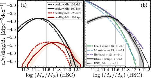
(a) Impact of using M⋆, 100kpc on the galaxy SMF. Dashed lines correspond to the observed volume density distribution computed using M⋆, cModel, whereas solid lines correspond to the distribution computed using M⋆, 100kpc. We do not apply any completeness correction to the distributions here. We separate our HSC sample into centrals in haloes more massive than log (M200b/M⊙)∼14.2 (red lines) and centrals in haloes with log (M200b/M⊙)<14.0 (black lines). The impact on the SMF can exceed 0.2 dex for massive central galaxies in very massive haloes. (b) The M⋆ volume density distributions of massive HSC galaxies, using both M⋆, 100kpc (black solid line) and M⋆, Max (black dotted line). Vertical lines on both plots highlight the log (M⋆, 100kpc/M⊙)=11.6 mass limit. The grey shaded region shows the resampling error on the HSC SMF plus an additional 20 per cent uncertainty to account for the fact that we do not include satellite galaxies and that we fail to extract a 1D profile for ∼10 per cent of our galaxies. These issues will be addressed in forthcoming work (Huang et al. in preparation). We compare our results with previous studies: (1) SDSS galaxies at z ∼ 0.1 from Bernardi et al. (2017) with M⋆ values based on photometry from 2D Sérsic +Exponential model fitting (purple); (2) SDSS galaxies at z ∼ 0.1 from Moustakas et al. (2013) based on improved SDSS cModel photometry (blue); and (3) S82-MGC galaxies at 0.15 < z < 0.43 from Leauthaud et al. (2016) based on PSF-matched SDSS–UKIDSS photometry (green).
The left-hand panel of Fig. 5 show the volume density distributions (referred to as SMF for simplicity) of massive galaxies using M⋆, cModel and M⋆, 100kpc for both the cenHighMh and cenLowMh samples. As shown in Fig. 3, the mass-dependent differences between these two measurements lead to noticeable differences in SMF at high-M⋆ end. cModel photometry leads to underestimation of volume density at the high-M⋆ end of SMF. More importantly, it shows that the impact of missing M⋆ becomes more significant for central galaxies in very massive haloes. We demonstrate that this occurs because galaxies in more massive haloes have more extended stellar envelopes than those in lower mass haloes at fixed M⋆, 100kpc in Huang et al. (in preparation). On the right-hand panel of Fig. 5, we also compare the SMFs using M⋆, 100kpc and M⋆, Max. As mentioned in Section 4.2, M⋆, 100kpc is still a lower limit of the total M⋆ of these massive galaxies, and M⋆, Max helps us check how much M⋆ could be left out. Although there is still visible difference at the high-M⋆ end, the impact of going from M⋆, 100kpc to M⋆, Max is relatively small. It suggests that M⋆, 100kpc captures the majority of the total M⋆. Here, we do not attempt to apply any completeness correction, so the SMFs turn over at the low-M⋆ end. For now, we add a constant ∼20 per cent uncertainty to the SMF to account for the satellite galaxies and the galaxies for which we fail to extract 1D profiles (see Appendix B), although these uncertainties should be smaller at high-M⋆ end.
On the right-hand panel of Fig. 5, we also compare our SMFs with the following works:
The SMF of 0.15 < z < 0.30 galaxies from the S82-MGC sample (Leauthaud et al. 2016), where M⋆ is based on PSF-matched aperture photometry and iSEDfit fitting using BC03 model. We account for the 0.08 dex average difference with the FSPS ones seen in the Appendix C
The SMF for the SDSS–GALEX sample at z ∼ 0.1 using SDSS cModel photometry and iSEDfit stellar mass based on similar assumptions [see Moustakas et al. (2013) for details].
The SMF for z ∼ 0.1 SDSS galaxies using 2D SerExp models14(Bernardi et al. 2013; Meert, Vikram & Bernardi 2015) and stellar mass by Mendel et al. (2014).15(See Bernardi et al. 2017 for details.)
Due to several systematics (see e.g. Bernardi et al. 2013, 2017), we do not attempt to perform detailed comparisons among these SMFs. We are currently working to address these issues in Huang et al. (in preparation). Here, we simply note that the HSC M⋆, 100kpc SMF is closer to the one derived by Bernardi et al. (2017) using SDSS data at z ∼ 0.1 and the SerExp model. Meanwhile, the differences between the HSC M⋆, 100kpc SMF with the others are likely caused by the photometric methods: SDSS cModel and small-aperture photometry underestimate M⋆ of massive galaxies. Even before a more in-depth study, it already illustrates an important issue: It is crucial to understand the impacts from photometric data and methods on the estimates of SMF before using HSC M⋆, 100kpc SMF to study galaxy evolution or comparing it with predictions from models and simulation. This is particularly relevant since a method like cModel will still be widely adopted in ongoing and future imaging surveys.
6.2 Surface mass density profiles
6.2.1 General trends and comparison with previous work
Previous work on the structural evolution of massive galaxies has often focused on scaling relations such as the ‘M⋆–size’ relation. We argue that by comparing μ⋆ profiles directly, we can capture more information than afforded by the M⋆–size relation. The comparison also has the advantage that it bypasses difficult questions about how to accurately define and measure galaxy ‘sizes’ and ‘masses’.
Fig. 6 shows the median μ⋆ profiles of massive central galaxies at 0.3 < z < 0.5 in three M⋆, 100kpc bins. These median profiles along with their uncertainties are derived using the bootstrap resampling method. Note that our sample is not complete in the lowest M⋆, 100kpc bin, although the median μ⋆ profile may not be significantly affected. As shown in the left-hand panel of Fig. 6, we can confidently trace the μ⋆ profiles of these massive galaxies out to 100 kpc individually. At large scales, some of our μ⋆ profiles show signs of unphysical truncation and fluctuation related to inaccurate sky subtraction. In this paper, we do not use profiles beyond 100 kpc, even though the median μ⋆ profiles for the two most massive bins behave reasonably well out to ∼200 kpc.
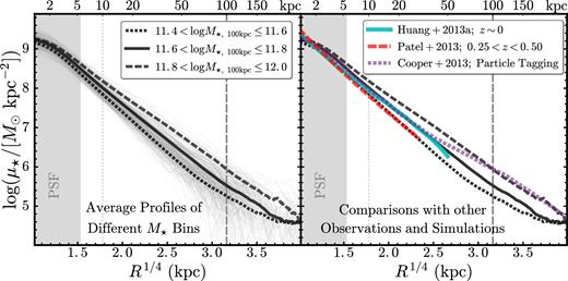
Left: median μ⋆ profiles in three total stellar mass bins. Thin grey lines in the background show a random subset of individual profiles. The scatter between the thin grey lines reflects the true scatter in the profiles of massive galaxies (not measurement error). The shaded region highlights the region that is most strongly affected by the seeing. Two vertical lines indicate 10 kpc (thin, dotted line) and 100 kpc (thick, dashed line). Right: comparison between our μ⋆ profiles, previous observations, and simulations. The solid cyan line shows the median profile of massive elliptical galaxies at z ∼ 0 from Huang et al. (2013a). The red long-dashed line shows the median profile of massive galaxies at 0.25 ≤ z < 0.50 observed by HST from Patel et al. (2013). The purple short-dashed line shows the median radial stellar distributions in massive haloes from simulation using the particle tagging method (Cooper et al. 2013).
From Fig. 6, we can see the galaxies in our sample have homogeneous profiles on small radial scales. The amplitude of μ⋆ increases with galaxy mass on 10 kpc scales but the slope of μ⋆ remains similar. From previous work on this topic, we already know that the inner regions of massive elliptical galaxies display relatively uniform structural (e.g. μ⋆ profile, isophotal shape: e.g. Lauer et al. 2007; Kormendy et al. 2009; Schombert 2015; and kinematic: e.g. Cappellari et al. 2013) properties. However, Fig. 6 reveals a significant diversity in the outer envelopes of massive galaxies. Given the S/N of HSC images at these surface brightness levels, the scatter shown in Fig. 6 corresponds to intrinsic scatter in the stellar envelopes of massive galaxies. Importantly, Fig. 6 shows that the global μ⋆ profiles of galaxies at these masses are clearly not self-similar out to 100 kpc and have outskirts with larger scatter.
In the right-hand side of Fig. 6, we compare our μ⋆ profiles with results from previous work. Most previous studies have focused on surface brightness profiles instead of mass density profiles. Results can also depend on the stacking technique or the model used to extract the profile (e.g. Tal & van Dokkum 2011; D'Souza et al. 2014). Huang et al. (2013a) derived μ⋆ profiles for a small sample of very nearby ellipticals (within 100 Mpc; median log (M⋆/M⊙) ∼11.3) based on relatively shallow images from the Carnegie–Irvine Galaxy Survey (Ho et al. 2011).16 This sample is at very low redshift (z < 0.02), and so the μ⋆ profiles from Huang et al. (2013a) galaxies are accurate to smaller scales (down to r = 1 kpc) than our HSC profiles. Our μ⋆ profiles show good agreement with the Huang et al. (2013a) sample in the radial range of overlap (out to 50 kpc). The median profiles from Huang et al. (2013a) only reach to ∼50 kpc for z < 0.02 massive galaxies, while our deep HSC images can reliably deliver individual μ⋆ profiles for z ∼ 0.4 galaxies out to at least 100 kpc.
Patel et al. (2013) extracted a median μ⋆ profile for massive ETGs at 0.25 < z < 0.50 using stacked Hubble Space Telescope [HST/Advanced Camera for Surveys (ACS)] images. These galaxies are selected at a constant cumulative number density and are thought to be the progenitors of z = 0 massive ETGs (e.g. Leja, van Dokkum & Franx 2013). The median M⋆ of the Patel et al. (2013) sample is ∼1011.2M⊙, which is lower than our lowest mass bin. However, Patel et al. (2013) uses the BC03 stellar population model, which leads to M⋆ that are roughly 0.1 dex lower than our FSPS estimates (see Appendix C). Furthermore, the Patel et al. (2013) images are shallower than ours which means that their M⋆ could still be underestimated due to missing light in the outskirts. Given these two considerations, it is reasonable to roughly compare the Patel et al. (2013) profile with the one in our lowest M⋆, 100kpc bin. The superb resolution of the HST/ACS images allows Patel et al. (2013) to accurately measure the μ⋆ profile down to 1 kpc without worrying about the smearing effect of seeing. The good agreement between our profiles and the ones derived from HST imaging demonstrates that our profiles are robust at r ≥ 3 kpc; therefore, we can accurately measure M⋆, 10kpc.
Finally, we also compare our HSC profiles with the predicted median μ⋆ profile of central galaxies in massive haloes (13.5 < log M200, c < 14.0) from a cosmological simulation where the μ⋆ profiles of galaxies are calculated using the particle tagging technique (e.g. Cooper et al. 2010). The simulated μ⋆ profile is affected by the resolution limit of the simulation in the inner region but is in good agreement with our median μ⋆ profile for the 11.6 < log (M⋆, 100kpc/M⊙) <11.8 bin within 40 kpc. However, when compared to our data for the 11.6 < log (M⋆, 100kpc/M⊙) <11.8 bin outside 40 kpc, the particle tagging method seems to predict an overly prominent stellar halo that has a much shallower outer slope.
Table 1 provides tabulated values for the median profiles that are displayed in Fig. 6. These profiles are also available here: http://www.ucolick.org/k~bundy/massivegalaxies. (The files will be made available after the paper is accepted.)
Average μ⋆ Profiles of Massive Galaxies in Different Stellar Mass Bins.
| Radius | [μ⋆]; Combined samples | [μ⋆]; M⋆, 100 kpc-matched | [μ⋆]; M⋆, 10 kpc-matched | ||||
|---|---|---|---|---|---|---|---|
| kpc | log (M⊙/kpc2) | log (M⊙/kpc2) | log (M⊙/kpc2) | ||||
| |$\log \frac{M_{\star ,100\mathrm{kpc}}}{M_{\odot }}\in$|[11.4, 11.6] | [11.6, 11.8] | [11.8, 12.0] | cenHighMh | cenLowMh | cenHighMh | cenLowMh | |
| (1) | (2) | (3) | (4) | (5) | (6) | (7) | (8) |
| 0.0 | |$9.23^{+0.00 }_{ -0.00}$| | |$9.31^{+0.00 }_{ -0.01}$| | |$9.32^{+0.01 }_{ -0.01}$| | |$9.31^{+0.02 }_{ -0.02}$| | |$9.34^{+0.01 }_{ -0.01}$| | |$9.31^{+0.02 }_{ -0.02}$| | |$9.34^{+0.02 }_{ -0.02}$| |
| 0.6 | |$9.20^{+0.00 }_{ -0.00}$| | |$9.28^{+0.00 }_{ -0.01}$| | |$9.29^{+0.01 }_{ -0.01}$| | |$9.27^{+0.02 }_{ -0.02}$| | |$9.31^{+0.01 }_{ -0.01}$| | |$9.28^{+0.02 }_{ -0.02}$| | |$9.31^{+0.02 }_{ -0.02}$| |
| 1.0 | |$9.16^{+0.00 }_{ -0.00}$| | |$9.24^{+0.00 }_{ -0.00}$| | |$9.26^{+0.01 }_{ -0.01}$| | |$9.24^{+0.02 }_{ -0.02}$| | |$9.27^{+0.01 }_{ -0.01}$| | |$9.25^{+0.02 }_{ -0.02}$| | |$9.27^{+0.02 }_{ -0.02}$| |
| 1.4 | |$9.12^{+0.00 }_{ -0.00}$| | |$9.20^{+0.00 }_{ -0.00}$| | |$9.23^{+0.01 }_{ -0.01}$| | |$9.20^{+0.02 }_{ -0.02}$| | |$9.23^{+0.01 }_{ -0.01}$| | |$9.21^{+0.02 }_{ -0.01}$| | |$9.23^{+0.02 }_{ -0.01}$| |
| 1.7 | |$9.06^{+0.00 }_{ -0.00}$| | |$9.15^{+0.00 }_{ -0.00}$| | |$9.19^{+0.01 }_{ -0.01}$| | |$9.15^{+0.02 }_{ -0.02}$| | |$9.19^{+0.01 }_{ -0.01}$| | |$9.16^{+0.01 }_{ -0.01}$| | |$9.18^{+0.01 }_{ -0.01}$| |
| 2.0 | |$9.00^{+0.00 }_{ -0.00}$| | |$9.10^{+0.00 }_{ -0.00}$| | |$9.15^{+0.01 }_{ -0.01}$| | |$9.09^{+0.01 }_{ -0.02}$| | |$9.13^{+0.01 }_{ -0.01}$| | |$9.11^{+0.01 }_{ -0.01}$| | |$9.12^{+0.01 }_{ -0.01}$| |
| 2.4 | |$8.93^{+0.00 }_{ -0.00}$| | |$9.03^{+0.00 }_{ -0.00}$| | |$9.09^{+0.01 }_{ -0.01}$| | |$9.03^{+0.02 }_{ -0.02}$| | |$9.07^{+0.01 }_{ -0.01}$| | |$9.05^{+0.01 }_{ -0.01}$| | |$9.05^{+0.01 }_{ -0.01}$| |
| 2.7 | |$8.87^{+0.00 }_{ -0.00}$| | |$8.97^{+0.00 }_{ -0.00}$| | |$9.04^{+0.01 }_{ -0.01}$| | |$8.97^{+0.01 }_{ -0.01}$| | |$9.01^{+0.01 }_{ -0.01}$| | |$9.00^{+0.01 }_{ -0.01}$| | |$8.99^{+0.01 }_{ -0.01}$| |
| 3.0 | |$8.80^{+0.00 }_{ -0.00}$| | |$8.90^{+0.00 }_{ -0.00}$| | |$8.98^{+0.01 }_{ -0.01}$| | |$8.90^{+0.01 }_{ -0.01}$| | |$8.95^{+0.01 }_{ -0.01}$| | |$8.93^{+0.01 }_{ -0.01}$| | |$8.92^{+0.01 }_{ -0.01}$| |
| 3.4 | |$8.72^{+0.00 }_{ -0.00}$| | |$8.83^{+0.00 }_{ -0.00}$| | |$8.92^{+0.01 }_{ -0.01}$| | |$8.83^{+0.01 }_{ -0.01}$| | |$8.88^{+0.01 }_{ -0.01}$| | |$8.86^{+0.01 }_{ -0.01}$| | |$8.85^{+0.01 }_{ -0.01}$| |
| 3.7 | |$8.66^{+0.00 }_{ -0.00}$| | |$8.78^{+0.00 }_{ -0.00}$| | |$8.87^{+0.01 }_{ -0.01}$| | |$8.78^{+0.01 }_{ -0.01}$| | |$8.83^{+0.01 }_{ -0.01}$| | |$8.81^{+0.01 }_{ -0.01}$| | |$8.79^{+0.01 }_{ -0.01}$| |
| 4.1 | |$8.60^{+0.00 }_{ -0.00}$| | |$8.72^{+0.00 }_{ -0.00}$| | |$8.82^{+0.01 }_{ -0.01}$| | |$8.72^{+0.01 }_{ -0.01}$| | |$8.77^{+0.01 }_{ -0.01}$| | |$8.76^{+0.01 }_{ -0.01}$| | |$8.73^{+0.01 }_{ -0.01}$| |
| 4.4 | |$8.54^{+0.00 }_{ -0.00}$| | |$8.66^{+0.00 }_{ -0.00}$| | |$8.77^{+0.01 }_{ -0.01}$| | |$8.66^{+0.01 }_{ -0.01}$| | |$8.72^{+0.01 }_{ -0.01}$| | |$8.70^{+0.01 }_{ -0.01}$| | |$8.67^{+0.01 }_{ -0.01}$| |
| 4.8 | |$8.48^{+0.00 }_{ -0.00}$| | |$8.60^{+0.00 }_{ -0.00}$| | |$8.71^{+0.01 }_{ -0.01}$| | |$8.60^{+0.01 }_{ -0.01}$| | |$8.66^{+0.01 }_{ -0.01}$| | |$8.65^{+0.01 }_{ -0.01}$| | |$8.61^{+0.01 }_{ -0.01}$| |
| 6.2 | |$8.26^{+0.00 }_{ -0.00}$| | |$8.40^{+0.00 }_{ -0.00}$| | |$8.53^{+0.01 }_{ -0.01}$| | |$8.41^{+0.01 }_{ -0.01}$| | |$8.46^{+0.01 }_{ -0.01}$| | |$8.46^{+0.02 }_{ -0.02}$| | |$8.40^{+0.02 }_{ -0.02}$| |
| 7.6 | |$8.09^{+0.00 }_{ -0.00}$| | |$8.24^{+0.00 }_{ -0.00}$| | |$8.39^{+0.01 }_{ -0.01}$| | |$8.27^{+0.01 }_{ -0.01}$| | |$8.31^{+0.01 }_{ -0.01}$| | |$8.31^{+0.02 }_{ -0.02}$| | |$8.23^{+0.02 }_{ -0.02}$| |
| 9.0 | |$7.95^{+0.00 }_{ -0.00}$| | |$8.10^{+0.00 }_{ -0.00}$| | |$8.27^{+0.01 }_{ -0.01}$| | |$8.14^{+0.02 }_{ -0.02}$| | |$8.18^{+0.01 }_{ -0.01}$| | |$8.19^{+0.02 }_{ -0.02}$| | |$8.09^{+0.02 }_{ -0.02}$| |
| 10.3 | |$7.82^{+0.00 }_{ -0.00}$| | |$7.99^{+0.00 }_{ -0.00}$| | |$8.16^{+0.01 }_{ -0.01}$| | |$8.03^{+0.02 }_{ -0.01}$| | |$8.06^{+0.01 }_{ -0.01}$| | |$8.09^{+0.02 }_{ -0.02}$| | |$7.97^{+0.02 }_{ -0.02}$| |
| 11.7 | |$7.70^{+0.00 }_{ -0.00}$| | |$7.88^{+0.00 }_{ -0.00}$| | |$8.06^{+0.01 }_{ -0.01}$| | |$7.93^{+0.02 }_{ -0.02}$| | |$7.96^{+0.01 }_{ -0.01}$| | |$7.99^{+0.02 }_{ -0.02}$| | |$7.85^{+0.02 }_{ -0.02}$| |
| 13.0 | |$7.60^{+0.00 }_{ -0.00}$| | |$7.78^{+0.00 }_{ -0.00}$| | |$7.98^{+0.01 }_{ -0.01}$| | |$7.85^{+0.02 }_{ -0.02}$| | |$7.87^{+0.01 }_{ -0.01}$| | |$7.90^{+0.02 }_{ -0.02}$| | |$7.75^{+0.02 }_{ -0.02}$| |
| 14.5 | |$7.50^{+0.00 }_{ -0.00}$| | |$7.69^{+0.00 }_{ -0.00}$| | |$7.90^{+0.01 }_{ -0.01}$| | |$7.76^{+0.02 }_{ -0.02}$| | |$7.78^{+0.01 }_{ -0.01}$| | |$7.82^{+0.02 }_{ -0.02}$| | |$7.65^{+0.02 }_{ -0.02}$| |
| 16.0 | |$7.39^{+0.00 }_{ -0.00}$| | |$7.60^{+0.00 }_{ -0.00}$| | |$7.82^{+0.01 }_{ -0.01}$| | |$7.68^{+0.02 }_{ -0.02}$| | |$7.69^{+0.01 }_{ -0.01}$| | |$7.74^{+0.02 }_{ -0.03}$| | |$7.56^{+0.02 }_{ -0.03}$| |
| 17.3 | |$7.31^{+0.00 }_{ -0.00}$| | |$7.52^{+0.00 }_{ -0.00}$| | |$7.76^{+0.01 }_{ -0.01}$| | |$7.61^{+0.02 }_{ -0.02}$| | |$7.62^{+0.01 }_{ -0.01}$| | |$7.67^{+0.03 }_{ -0.03}$| | |$7.48^{+0.03 }_{ -0.03}$| |
| 18.7 | |$7.23^{+0.00 }_{ -0.00}$| | |$7.45^{+0.00 }_{ -0.00}$| | |$7.69^{+0.01 }_{ -0.01}$| | |$7.55^{+0.02 }_{ -0.02}$| | |$7.55^{+0.01 }_{ -0.01}$| | |$7.61^{+0.03 }_{ -0.03}$| | |$7.40^{+0.03 }_{ -0.03}$| |
| 22.6 | |$7.02^{+0.00 }_{ -0.00}$| | |$7.27^{+0.00 }_{ -0.00}$| | |$7.54^{+0.01 }_{ -0.01}$| | |$7.38^{+0.02 }_{ -0.02}$| | |$7.37^{+0.01 }_{ -0.01}$| | |$7.45^{+0.03 }_{ -0.03}$| | |$7.21^{+0.03 }_{ -0.03}$| |
| 26.1 | |$6.86^{+0.00 }_{ -0.00}$| | |$7.12^{+0.00 }_{ -0.00}$| | |$7.41^{+0.01 }_{ -0.01}$| | |$7.25^{+0.02 }_{ -0.02}$| | |$7.24^{+0.01 }_{ -0.01}$| | |$7.32^{+0.03 }_{ -0.03}$| | |$7.05^{+0.03 }_{ -0.03}$| |
| 30.0 | |$6.70^{+0.00 }_{ -0.00}$| | |$6.98^{+0.00 }_{ -0.00}$| | |$7.29^{+0.01 }_{ -0.01}$| | |$7.13^{+0.03 }_{ -0.02}$| | |$7.10^{+0.01 }_{ -0.01}$| | |$7.20^{+0.03 }_{ -0.04}$| | |$6.90^{+0.03 }_{ -0.04}$| |
| 33.7 | |$6.55^{+0.00 }_{ -0.00}$| | |$6.85^{+0.01 }_{ -0.01}$| | |$7.18^{+0.01 }_{ -0.01}$| | |$7.01^{+0.03 }_{ -0.03}$| | |$6.98^{+0.01 }_{ -0.01}$| | |$7.09^{+0.03 }_{ -0.03}$| | |$6.76^{+0.03 }_{ -0.03}$| |
| 37.8 | |$6.41^{+0.00 }_{ -0.00}$| | |$6.72^{+0.01 }_{ -0.01}$| | |$7.07^{+0.01 }_{ -0.01}$| | |$6.90^{+0.03 }_{ -0.03}$| | |$6.85^{+0.01 }_{ -0.01}$| | |$6.98^{+0.04 }_{ -0.04}$| | |$6.63^{+0.04 }_{ -0.04}$| |
| 41.6 | |$6.29^{+0.01 }_{ -0.01}$| | |$6.61^{+0.01 }_{ -0.01}$| | |$6.98^{+0.01 }_{ -0.01}$| | |$6.81^{+0.03 }_{ -0.03}$| | |$6.75^{+0.01 }_{ -0.01}$| | |$6.89^{+0.04 }_{ -0.04}$| | |$6.51^{+0.04 }_{ -0.04}$| |
| 45.7 | |$6.17^{+0.01 }_{ -0.01}$| | |$6.50^{+0.01 }_{ -0.01}$| | |$6.88^{+0.01 }_{ -0.01}$| | |$6.71^{+0.03 }_{ -0.03}$| | |$6.64^{+0.01 }_{ -0.01}$| | |$6.79^{+0.04 }_{ -0.04}$| | |$6.39^{+0.04 }_{ -0.04}$| |
| 49.3 | |$6.07^{+0.01 }_{ -0.01}$| | |$6.41^{+0.01 }_{ -0.01}$| | |$6.80^{+0.01 }_{ -0.02}$| | |$6.62^{+0.03 }_{ -0.03}$| | |$6.56^{+0.01 }_{ -0.01}$| | |$6.70^{+0.04 }_{ -0.04}$| | |$6.30^{+0.04 }_{ -0.04}$| |
| 53.1 | |$5.98^{+0.01 }_{ -0.01}$| | |$6.33^{+0.01 }_{ -0.01}$| | |$6.71^{+0.02 }_{ -0.02}$| | |$6.55^{+0.03 }_{ -0.03}$| | |$6.46^{+0.01 }_{ -0.01}$| | |$6.64^{+0.04 }_{ -0.04}$| | |$6.21^{+0.04 }_{ -0.04}$| |
| 57.2 | |$5.88^{+0.01 }_{ -0.01}$| | |$6.24^{+0.01 }_{ -0.01}$| | |$6.63^{+0.02 }_{ -0.02}$| | |$6.47^{+0.04 }_{ -0.04}$| | |$6.37^{+0.01 }_{ -0.01}$| | |$6.56^{+0.04 }_{ -0.04}$| | |$6.11^{+0.04 }_{ -0.04}$| |
| 61.5 | |$5.79^{+0.01 }_{ -0.01}$| | |$6.15^{+0.01 }_{ -0.01}$| | |$6.55^{+0.02 }_{ -0.02}$| | |$6.39^{+0.04 }_{ -0.04}$| | |$6.29^{+0.01 }_{ -0.01}$| | |$6.49^{+0.04 }_{ -0.04}$| | |$6.03^{+0.04 }_{ -0.04}$| |
| 66.0 | |$5.70^{+0.01 }_{ -0.01}$| | |$6.05^{+0.01 }_{ -0.01}$| | |$6.47^{+0.02 }_{ -0.02}$| | |$6.32^{+0.04 }_{ -0.04}$| | |$6.20^{+0.01 }_{ -0.01}$| | |$6.37^{+0.05 }_{ -0.06}$| | |$5.94^{+0.05 }_{ -0.06}$| |
| 69.8 | |$5.64^{+0.01 }_{ -0.01}$| | |$5.98^{+0.01 }_{ -0.01}$| | |$6.40^{+0.02 }_{ -0.02}$| | |$6.25^{+0.04 }_{ -0.04}$| | |$6.12^{+0.02 }_{ -0.01}$| | |$6.35^{+0.04 }_{ -0.05}$| | |$5.87^{+0.04 }_{ -0.05}$| |
| 74.7 | |$5.56^{+0.01 }_{ -0.01}$| | |$5.89^{+0.01 }_{ -0.01}$| | |$6.32^{+0.02 }_{ -0.02}$| | |$6.18^{+0.04 }_{ -0.04}$| | |$6.04^{+0.02 }_{ -0.02}$| | |$6.28^{+0.05 }_{ -0.05}$| | |$5.79^{+0.05 }_{ -0.05}$| |
| 79.9 | |$5.49^{+0.01 }_{ -0.01}$| | |$5.81^{+0.01 }_{ -0.01}$| | |$6.24^{+0.02 }_{ -0.02}$| | |$6.12^{+0.04 }_{ -0.04}$| | |$5.96^{+0.02 }_{ -0.02}$| | |$6.20^{+0.05 }_{ -0.06}$| | |$5.72^{+0.05 }_{ -0.06}$| |
| 84.3 | |$5.43^{+0.01 }_{ -0.01}$| | |$5.74^{+0.01 }_{ -0.01}$| | |$6.18^{+0.02 }_{ -0.02}$| | |$6.05^{+0.04 }_{ -0.05}$| | |$5.89^{+0.02 }_{ -0.02}$| | |$6.16^{+0.05 }_{ -0.05}$| | |$5.65^{+0.05 }_{ -0.05}$| |
| 88.8 | |$5.38^{+0.01 }_{ -0.01}$| | |$5.67^{+0.01 }_{ -0.01}$| | |$6.11^{+0.02 }_{ -0.02}$| | |$5.99^{+0.05 }_{ -0.06}$| | |$5.81^{+0.02 }_{ -0.02}$| | |$6.08^{+0.05 }_{ -0.06}$| | |$5.58^{+0.05 }_{ -0.06}$| |
| 97.2 | |$5.29^{+0.01 }_{ -0.01}$| | |$5.56^{+0.01 }_{ -0.01}$| | |$5.98^{+0.02 }_{ -0.02}$| | |$5.92^{+0.04 }_{ -0.04}$| | |$5.69^{+0.02 }_{ -0.02}$| | |$5.99^{+0.05 }_{ -0.05}$| | |$5.47^{+0.05 }_{ -0.05}$| |
| 103.6 | |$5.21^{+0.01 }_{ -0.01}$| | |$5.49^{+0.01 }_{ -0.01}$| | |$5.89^{+0.03 }_{ -0.03}$| | |$5.84^{+0.05 }_{ -0.05}$| | |$5.62^{+0.02 }_{ -0.02}$| | |$5.94^{+0.05 }_{ -0.05}$| | |$5.39^{+0.05 }_{ -0.05}$| |
| 111.6 | |$5.14^{+0.01 }_{ -0.01}$| | |$5.40^{+0.01 }_{ -0.01}$| | |$5.79^{+0.03 }_{ -0.03}$| | |$5.78^{+0.05 }_{ -0.05}$| | |$5.54^{+0.02 }_{ -0.02}$| | |$5.87^{+0.05 }_{ -0.05}$| | |$5.32^{+0.05 }_{ -0.05}$| |
| 117.2 | |$5.10^{+0.01 }_{ -0.01}$| | |$5.36^{+0.01 }_{ -0.01}$| | |$5.72^{+0.03 }_{ -0.03}$| | |$5.72^{+0.05 }_{ -0.05}$| | |$5.47^{+0.02 }_{ -0.02}$| | |$5.82^{+0.05 }_{ -0.05}$| | |$5.29^{+0.05 }_{ -0.05}$| |
| 129.0 | |$5.00^{+0.01 }_{ -0.01}$| | |$5.25^{+0.02 }_{ -0.02}$| | |$5.61^{+0.03 }_{ -0.03}$| | |$5.64^{+0.05 }_{ -0.05}$| | |$5.36^{+0.02 }_{ -0.02}$| | |$5.74^{+0.05 }_{ -0.05}$| | |$5.21^{+0.05 }_{ -0.05}$| |
| 141.7 | |$4.89^{+0.02 }_{ -0.02}$| | |$5.13^{+0.02 }_{ -0.02}$| | |$5.49^{+0.03 }_{ -0.03}$| | |$5.58^{+0.05 }_{ -0.05}$| | |$5.23^{+0.03 }_{ -0.03}$| | |$5.66^{+0.05 }_{ -0.05}$| | |$5.09^{+0.05 }_{ -0.05}$| |
| 146.7 | |$4.85^{+0.02 }_{ -0.02}$| | |$5.10^{+0.02 }_{ -0.02}$| | |$5.46^{+0.03 }_{ -0.03}$| | |$5.51^{+0.06 }_{ -0.06}$| | |$5.19^{+0.03 }_{ -0.03}$| | |$5.61^{+0.05 }_{ -0.05}$| | |$5.03^{+0.05 }_{ -0.05}$| |
Notes. Average μ⋆ profiles of massive cenHighMh and cenLowMh galaxies in different samples:
Col. (1) Radius along the major axis in kpc.
Col. (2) Average μ⋆ profile for galaxies with 11.4 ≤log (M⋆, 100kpc/M⊙)<11.6 in the combined samples of cenHighMh and cenLowMh galaxies.
Col. (3) Average μ⋆ profile of combined samples in the mass bin of 11.6 ≤log (M⋆, 100kpc/M⊙)<11.8.
Col. (4) Average μ⋆ profile of combined samples in the mass bin of 11.8 ≤log (M⋆, 100kpc/M⊙)<12.0.
Col. (5) and Col. (6) are the average μ⋆ profiles of cenHighMh and cenLowMh galaxies in the M⋆, 100kpc-matched samples within 11.6 ≤log (M⋆, 100kpc/M⊙)<11.9.
Col. (7) and Col. (8) are the average μ⋆ profiles of cenHighMh and cenLowMh galaxies in the M⋆, 10kpc-matched samples within 11.2 ≤log (M⋆, 100kpc/M⊙)<11.6.
The upper and lower uncertainties of these average profiles vial bootstrap-resampling method are also displayed.
6.3 Ellipticity and colour profiles
Now we look into the ellipticity profile derived by Ellipse in i band and the g − r and g − i colour profiles (galactic extinction and k-corrected). The smearing effect of seeing makes the central isophotal shape rounder than the real value, while seeing differences between filters bias the central colour.17 On large scales, it is more difficult to extract reliable ellipticity and colour profiles out to 100 kpc because at low surface brightness levels, the isophotal shape becomes unstable and is easily affected by contamination. Colour profiles are also more difficult to extract out to large radial scales because getting the colour accurately depends on the background subtraction and the noise levels in both bands. In this paper, we focus on the median ellipticity and colour profiles between 8 and 60 kpc, where we can safely ignore the issues described above.
The left-hand panel of Fig. 7 shows the ellipticity profiles of massive galaxies and highlights the median profiles for the same three M⋆, 100kpc bins shown in Fig. 6. Our results are also compared with previous work based on image stacking techniques (the PSF-removed i-band results from Tal & van Dokkum (2011), and concentrated galaxies with 11.0 <log (M⋆/M⊙)<11.4 from D'Souza et al. (2015). As expected, ellipticity profiles from image stacking methods yield results that are more shallow than ellipticity profiles measured on a galaxy-by-galaxy basis. Uncertainties in how to align galaxies and the intrinsic isophotal twist can lead to this effect.
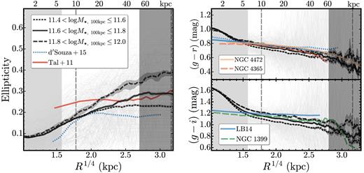
Radial profiles of the ellipticity and k-corrected rest-frame optical colours of massive galaxies in our sample. The general format of this figure is similar to Fig. 6. The left-hand panel displays ellipticity profiles, the upper right panel shows g − r colour profiles, and the lower right panel is for g − i colour profiles. We compare our results with those from (1) Tal & van Dokkum (2011) based on stacking large samples of LRGs in SDSS at z ∼ 0.4 (solid red line on the left-hand panel), (2) the results from a stacking analysis of nearby massive galaxies with high concentration index (C > 2.6) in D'Souza et al. (2014, blue dash lines on the left-hand and upper right panels), (3) and the average g − r and g − i colour profiles from a large sample of nearby elliptical galaxies in La Barbera et al. (2010, blue, solid lines on both right-hand panels). For colour profiles, we also compare with deep observations of a few nearby massive ETGs: the g − r colour profiles of NGC 4472 (Mihos et al. 2013) and NGC 4365 (Mihos et al. 2017), and the g − i profile of NGC 1399 (Iodice et al. 2016).
In general, we find that the ellipticities of massive galaxies slowly increase with radius. This trend can even be seen directly ‘by eye’ in HSC images (e.g. Fig. 1). More interestingly, the ellipticity profiles vary with M⋆, 100kpc: at ∼10 kpc, the median ellipticity (<0.2) is similar for all three redshift bins, but the ellipticity of the outer stellar halo increases with M⋆, 100kpc. Galaxies with log (M⋆, 100kpc/M⊙)>11.8 have median ellipticity profiles that become steeper at >10 kpc. The ellipticity of the outer profile steadily increases from e ≤ 0.2 to e ∼ 0.4 at 50–60 kpc.
This is consistent with studies of nearby massive galaxies using different methods (e.g. Porter, Schneider & Hoessel 1991; Gonzalez, Zabludoff & Zaritsky 2005; Zibetti et al. 2005; Huang et al. 2013a; Oh, Greene & Lackner 2017). For instance, Spavone et al. (2017) use very deep images of six nearby massive galaxies to show that their average ellipticity in g band also increases with radius in a similar fashion. However, to the best of our knowledge, our HSC results are the first to show clear evidence that: (1) the ellipticity of stellar halo in massive ETGs depends strongly on M⋆, 100kpc, and (2) the ellipticity of stellar halo also relates to the slope of the μ⋆ profile (see Figs 6 and 7; we will discuss this more in Huang et al. in preparation). As mentioned in Section 1, such a mass-dependent ellipticity profile could reveal more insights about the assembly of stellar haloes of massive galaxies.
Regarding the colour profiles, the right-hand panels of Fig. 7 show the k-corrected (g − r) and (g − i) colour profiles for all galaxies in our sample, together with the median profiles in three M⋆, 100kpc bins. We find that the median rest-frame (g − r) and (g − i) colour profiles present smooth and shallow negative colour gradients out to 50–60 kpc, as observed by many previous works (e.g. Carollo et al. 1993; La Barbera et al. 2012) and predicted by some simulations (e.g. Hirschmann et al. 2015). Meanwhile, there does not appear to be a significant M⋆ dependence in the gradient of rest-frame optical colours.
We also compare our results with the stacked colour profiles from La Barbera et al. (2010)18 and D'Souza et al. (2014). The median colour profiles from HSC images are systematically steeper than the stacked SDSS ones. Considering differences in the response curves between HSC and SDSS filters, together with the uncertainties of colour measurements, the HSC (g − r) colour profiles are in fairly good agreement with those from SDSS. However, the (g − i) profiles of HSC galaxies are steeper compared to SDSS. The SDSS i band suffers from the so-called ‘red-halo’ effect (e.g. Wu et al. 2005, Tal & van Dokkum 2011). This is likely due to the fact that the SDSS i-band PSF has a more prominent wing than other bands. Because the PSF model does not capture these wings, more flux is artificially distributed to the outskirts, which leads to seemingly redder colours in the low surface brightness outskirts of galaxies. Because HSC uses thick CCDs, HSC i-band images do not suffer from this effect and can be used to determine galaxy colours with higher accuracy. Fairly steep colour profiles have been observed in several very nearby massive ETGs. Fig. 7 shows the g − r colour profiles of NGC 4472 (Mihos et al. 2013) and NGC 4365 (Mihos et al. 2017),19 and the g − i profile of NGC 1399 (Iodice et al. 2016). These individual profiles display colour gradients similar to our HSC sample.
It is worth mentioning that the individual colour profiles still show large scatter and unphysical trends in the outskirt. The colour profile in the low-surface brightness region is very sensitive to the noise level, contamination of other objects, and uncertainties in background subtraction. The HSC g-band images are relatively shallower and the backgrounds from the two bands are not jointly constrained. Therefore, we only show the average colour profiles here, and will conduct more careful study of the colour profiles in Huang et al. (in preparation).
7 DISCUSSION
We have used data from the HSC survey that is both simultaneously deep and wide to trace the stellar mass distributions of 0.3 < z < 0.5 massive galaxies out to >100 kpc and to reveal the mass-dependent nature of their stellar haloes. Here, we briefly discuss the scientific implications of our results.
7.1 The formation of massive galaxies and the assembly of their outer haloes
We find that the outer haloes of massive elliptical galaxies grow more prominent and more elliptical with increasing stellar mass. According to the two-phase formation scenario, the inner 5–10 kpc of these massive central galaxies are formed at z > 1 during an intense period of in situ star formation. The outskirts of massive galaxies are then built up through a more gradual second phase of evolution (the ex situ phase) that is dominated by mass assembly via accretions. Non-dissipative mergers, especially minor mergers,20 deposit stars mostly in the outskirts of centrals and do not have a large impact on the central μ⋆ profile (e.g. Boylan-Kolchin, Ma & Quataert 2008; Oogi & Habe 2013; Bédorf & Portegies Zwart 2013). Given the stochastic nature of the merging process, it is easy to understand why the μ⋆ profiles of massive galaxies are similar in the inner region but show a large scatter in the outer region.
State of the art hydrodynamic simulations of massive galaxy formation predict that the fraction of accreted stars should strongly increase with stellar mass and that for very massive galaxies, the ex situ may reach up to 50–90 per cent of the total galaxy mass (e.g. Oser et al. 2010; Cooper et al. 2013; Dubois et al. 2013; Lee & Yi 2013; Hirschmann et al. 2015; Rodriguez-Gomez et al. 2016).
This picture is supported by our observations that massive galaxies display more prominent stellar haloes as well as by their negative colour gradients. The fact that the outskirts of these galaxies are slightly bluer than the inner regions is consistent with the picture that stellar haloes are built up by a series of minor mergers (average merger mass ratio between 1:3 and 1:10; e.g. Huang et al. 2016b) because less massive ETGs are typically bluer.
Also according to this picture, the shape of the stellar halo should preserve information about the merging history and possibly even about the shape of the dark matter halo. Simulations show the shape of the stellar and dark matter haloes are closely correlated (e.g. Wu et al. 2014) for slowly rotating massive ETGs having undergone multiple minor mergers. The more elongated outer halo and the trend between the ellipticity profile and stellar mass may reflect the orbital properties of an accreted satellite. In simulations, satellite orbits become more radial for more massive haloes (e.g. Murante et al. 2007; Wetzel 2011; Jiang et al. 2015. Satellites infalling along radial orbits may help to form elongated stellar haloes. In principle, these results may explain the trend that we see. However, in contrast, simulation from Wu et al. (2014) predict that more massive galaxies should have rounder outskirts, which is the opposite trend compared to HSC. This difference warrants further investigation.
At larger scales, the distribution of satellite galaxies in massive haloes is found to be aligned with the major axis of the central galaxy (e.g. Brainerd 2005; Yang et al. 2006; Niederste-Ostholt et al. 2010; Huang et al. 2016a). This alignment signal is found to be stronger for more luminous galaxies living in more massive haloes (e.g. Hirata et al. 2007). The fact that more massive central galaxies have steeper ellipticity profiles and become increasingly more elongated in the outskirt may be due to such alignment. Moreover, the shape of the dark matter halo can be estimated by analysing satellite distributions and weak-lensing profiles (Clampitt & Jain 2016). It is interesting to point out that the most recent measurement by Shin et al. (2017) around SDSS clusters shows a halo axis ratio of ∼0.55, which is only slightly more elongated than the stellar halo of galaxies in our highest M⋆, 100kpc bin.
7.2 Aperture masses as proxies of the in situ and accreted stars
As mentioned in Section 1, hydrodynamic simulations often predict that the faction of ex situ stars increase with total stellar mass. However, it is still extremely difficult to separate the in situ and ex situ components observationally, despite the fact that it is the most important theoretical prediction to be verified.
Recent deep surveys of nearby disc galaxies have started to provide constraints on their stellar haloes (e.g. Courteau et al. 2011; Merritt et al. 2016; Harmsen et al. 2017),21 as it is relatively easier to decompose the stellar halo component. As for massive ETGs, limited observational constraints still mainly depend on multicomponent model fitting and/or image stacking analyses (e.g. Gonzalez, Zaritsky & Zabludoff 2007; Huang et al. 2013a; D'Souza et al. 2014; Spavone et al. 2017). In this work, we propose that M⋆ values computed within different fixed physical elliptical apertures are worth exploring as proxies of the ex situ fraction. We propose to use the mass within 10 kpc (M⋆, 10kpc) and 100 kpc (M⋆, 100kpc) as proxies for the in situ component and for the total M⋆.
On the left-hand panel of Fig. 8, we show the relation between M⋆, 100kpc and the fraction of mass between 10 and 100 kpc (as a proxy of the mass of the accreted component). We compare this with the fraction of ex situ stars predicted by the Illustris simulation (Rodriguez-Gomez et al. 2016). We find that our proxy for the accreted mass component correlates strongly with M⋆, 100kpc and that this relation is surprisingly consistent with predictions from Rodriguez-Gomez et al. (2016). Given the limitations of the Illustris simulation and the imperfect nature of our ex situ fraction proxy, the almost perfect agreement seen in Fig. 8 may well be a coincidence. However, it is encouraging to see that our simple proxy for the fraction of ex situ stars seems to match both the slope and the scatter of the predicted relation. There are other hydrodynamic simulations that predict significantly different ex situ fractions compared to Illustris (e.g. Lackner et al. 2012; Qu et al. 2017). Furthermore, a few known issues in the original Illustris simulation have been resolved in the new Illustris–TNG version (e.g. Genel et al. 2018; Pillepich et al. 2018. In future works (including Huang et al. in preparation), we will explore more comparisons with detailed predictions from new simulations to see how well we can trace ex situ fractions in massive galaxies using simple elliptical aperture masses.
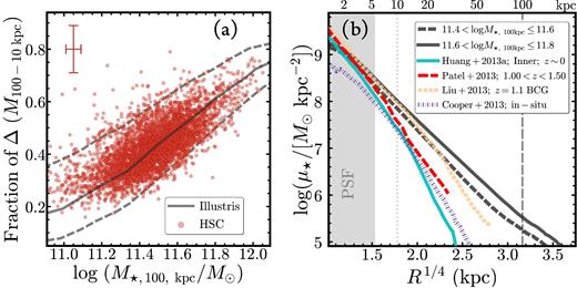
Left:ratio of the fraction of stars between 10 and 100 kpc to the total galaxy mass M⋆, 100kpc. We adopt this ratio as a proxy for the fraction of ex situ stars in our sample. Typical observational uncertainties are shown in the upper left hand corner. The solid grey line shows the predicted relation derived from the Illustris simulation at z = 0 (fig. 4 in Rodriguez-Gomez et al. 2016). Regions between the grey dashed lines correspond to the range between the 16 and 84 percentile of the distribution. Right: comparison between our median μ⋆ profiles with the inner component of the structural decomposition of massive elliptical galaxies at z < 0.02 from Huang et al. (2013a, , cyan, solid). At higher redshifts, the μ⋆ profiles of massive galaxies should be dominated by the in situ component. We compare our profiles with the median μ⋆ profile of massive galaxies at 1.0 < z < 1.5 from HST observations (Patel et al. 2013, , red, dashed). Both these comparisons suggest that the μ⋆ profile within 10 kpc is dominated by in situ stars, but there are already contributions from the accreted stars at very high M⋆ end. We also compare with the μ⋆ profile of a very massive cD galaxy at z ∼ 1.1 discovered by Liu et al. (2013, , yellow, dashed) in the Hubble Ultra Deep Field. It is likely that this object will grow into one of the very massive central galaxies in our sample. It is interesting to see that its μ⋆ profile is very similar to the HSC profile of the most massive M⋆, 100kpc bin in the inner ∼20 kpc, so the resulting growth should mostly happen in the outskirt.
Here, we further compare our μ⋆ profiles with (1) the profiles of the in situ component estimated from different ways, and (2) profiles of high-redshift massive galaxies that should be dominated by the in situ component. In particular, we compare with the following:
The median μ⋆ profiles of massive ETGs at 1.0 < z < 1.5 from Patel et al. (2013). These are considered to be the progenitors of ∼1011.5M⊙ ETGs at z = 0 and their inner region should be dominated by in situ stars.
The inner component of z ∼ 0 ellipticals from the 2D decomposition of Huang et al. (2013a). Huang et al. (2013b) show that this inner component is structurally similar to the compact ‘red nuggets’ at high-z.
The in situ components of simulated central galaxies in massive haloes from Cooper et al. (2013, , the inner ∼5 kpc is quite uncertain due to the resolution). These μ⋆ profiles are generated using the particle tagging method (see Cooper et al. 2010)
Although these simple comparisons support the idea that M⋆, 10kpc mainly consists of in situ stars. whereas mass at R > 15–20 kpc is dominated by ex situ component, they also show that the in situ component could extend beyond 10 kpc,22 and a fraction of mass within 10 kpc could also come from accretion (see also Rodriguez-Gomez et al. 2016). This is certainly the limitation for using aperture masses as proxies of in situ and ex situ masses. In other works (e.g. Huang et al. 2013a; Spavone et al. 2017), the outer component from image decomposition is treated as proxy of the ex situ component. Since such a photometric component extends to the centre of the galaxy and can reach a radius much larger than 100 kpc, it can lead to a higher ex situ fraction than ours (e.g. Spavone et al. 2017). It will be very interesting to apply a similar decomposition method to both the HSC images and the simulated massive galaxies to help us determine the best tracer of the in situ and ex situ mass.
We also compare our results with a uniquely massive galaxy at high redshift: a log (M⋆/M⊙)∼1011.4M⊙ galaxy with a distinctive ‘cD’-like envelope at z ∼ 1.1 (Liu et al. 2013). This high-redshift galaxy has a μ⋆ profile that follows the median μ⋆ profile of our 11.6 ≤log (M⋆, 100kpc/M⊙)<11.8 sample nicely at R < 40 kpc, but the profile becomes much steeper in the outskirt. The steeper profile suggests that, while the very outskirt of the stellar halo is still being assembled, some massive high-z galaxies may already have a significant fraction of ex situ stars. In future works (including Huang et al. in preparation), we will also look into the redshift evolution of the outer μ⋆ profiles up to z ∼ 1.0 using both HSC and other observations. Comparisons with relevant simulations can also tell us how well we can trace the evolution of the ex situ fraction of stars using aperture masses.
8 SUMMARY AND CONCLUSIONS
In this work, we use deep images from the Subaru HSC survey to study how the projected stellar mass density profiles and other structural properties of massive central galaxies depend on their total stellar mass. With the help of this high-quality, wide-area data set, we directly map the stellar mass distributions of ∼7000 massive central galaxies at 0.3 < z < 0.5 out to >100 kpc without resorting to stacking techniques. We group massive central galaxies into two categories based on their host halo mass (M200b|$\, \buildrel> \over {\sim } \,$|1014.0M⊙ and M200b|$\, \buildrel< \over {\sim } \,$|1014M⊙) and three bins of M⋆, 100kpc. Our main results are:
We show that the μ⋆ profiles of massive galaxies are relatively homogenous within 10–20 kpc. However, there is large scatter in outer profiles of massive galaxies. Galaxies with higher M⋆, 100kpc show more prominent stellar haloes and have shallower outer μ⋆ slopes. Assuming that stellar haloes are dominated by accreted stars, this result is consistent with the two-phase formation picture of massive galaxies.
We show that, on average, massive galaxies have positive ellipticity gradients out to at least 60 kpc. The average ellipticity profile also depends on M⋆, 100kpc: More massive galaxies tend to have steeper ellipticity gradients and become more elongated in stellar haloes.
On the other hand, although massive galaxies in all three M⋆, 100kpc bins show clearly negative average colour gradients out to 60 kpc, the average (g − r) and (g − i) colour gradients do not show clear dependence on M⋆, 100kpc.
We propose that, under reasonable assumptions, stellar masses within different physical apertures could be used to trace the in situ and ex situ components. Here, we show that M⋆, 10kpc and the M⋆ between 10 and 100 kpc could be promising proxies for the two physical components, and can recover the trend between stellar mass and ex situ fraction from simulation.
We find that the ‘total’ M⋆ of these massive galaxies can be significantly underestimated with shallow imaging data such as SDSS and/or oversimplified model assumptions (e.g. the cModel or single-Sérsic ). In contrast to previous work, our results do not depend on stacking or any parametric models. Moreover, the degree to which stellar mass is underestimated depends on M⋆, 100kpc. A simple model misses more light for massive galaxies because they have more extended envelopes. There is also an M200b dependence of this effect, and simple luminosity estimates will miss more light for BCGs in more massive haloes compared to centrals in less massive haloes. These effects need to be carefully taken into account when discussing topics such as the evolution of the galaxy SMF.
These results highlight the advantages of wide-area, deep, and high-quality imaging for studying the evolution of massive galaxies. At present, the HSC survey has already doubled its sky coverage to ∼200 deg2 and provides a much larger sample of massive central galaxies. In the near future, we will extend this work to lower M⋆, 100kpc by using photometric redshifts, and we will also apply 2D photometric methods (e.g. Huang et al. 2013a) to take advantage of the multiwavelength nature of the HSC survey (e.g. Huang et al. 2016b). Our current work can also be combined with weak-lensing measurements of the dark matter haloes of massive galaxies, and physical insights into the assembly histories of these galaxies can be gained by comparing the measurements with cosmological hydrosimulations such as Illustris (Vogelsberger et al. 2014, Genel et al. 2014), Evolution and Assembly of GaLaxies and their Environments (EAGLE) (Schaye et al. 2015, Crain et al. 2015), or Horizon–AGN (Dubois et al. 2014).
ACKNOWLEDGEMENTS
The authors thank Rachel Mandelbaum and Frank van den Bosch for insightful discussions and comments, Shun Saito for helping us estimate the fraction of satellite galaxies in our sample, and Feng-Shan Liu for sharing the μ⋆ profile of the z ∼ 1 brightest cluster galaxy from his work. This material is based upon work supported by the National Science Foundation under Grant No. 1714610.
The HSC collaboration includes the astronomical communities of Japan and Taiwan, and Princeton University. The HSC instrumentation and software were developed by National Astronomical Observatory of Japan (NAOJ), Kavli Institute for the Physics and Mathematics of the Universe (Kavli IPMU), University of Tokyo, High Energy Accelerator Research Organization (KEK), Academia Sinica Institute for Astronomy and Astrophysics in Taiwan (ASIAA), and Princeton University. Funding was contributed by the FIRST program from the Japanese Cabinet Office; Ministry of Education, Culture, Sports, Science and Technology; Japan Society for the Promotion of Science; Japan Science and Technology Agency (JST); Toray Science Foundation; NAOJ; Kavli IPMU; KEK; ASIAA; and Princeton University.
Funding for SDSS-III has been provided by Alfred P. Sloan Foundation, Participating Institutions, National Science Foundation, and U.S. Department of Energy. The SDSS-III website is http://www.sdss3.org. SDSS-III is managed by Astrophysical Research Consortium for the Participating Institutions of the SDSS-III Collaboration, which includes University of Arizona, Brazilian Participation Group, Brookhaven National Laboratory, University of Cambridge, University of Florida, the French Participation Group, German Participation Group, Instituto de Astrofisica de Canarias, Michigan State/Notre Dame/JINA Participation Group, Johns Hopkins University, Lawrence Berkeley National Laboratory, Max Planck Institute for Astrophysics, New Mexico State University, New York University, Ohio State University, Pennsylvania State University, University of Portsmouth, Princeton University, the Spanish Participation Group, University of Tokyo, University of Utah, Vanderbilt University, University of Virginia, University of Washington, and Yale University.
The Pan-STARRS1 Surveys (PS1) have been made possible through contributions of Institute for Astronomy; University of Hawaii; Pan-STARRS Project Office; Max-Planck Society and its participating institutes: Max Planck Institute for Astronomy, Heidelberg, and the Max Planck Institute for Extraterrestrial Physics, Garching; Johns Hopkins University; Durham University; University of Edinburgh; Queen's University Belfast; Harvard–Smithsonian Center for Astrophysics; Las Cumbres Observatory Global Telescope Network Incorporated; National Central University of Taiwan; Space Telescope Science Institute; National Aeronautics and Space Administration under Grant No. NNX08AR22G issued through the Planetary Science Division of the NASA Science Mission Directorate; National Science Foundation under Grant No. AST-1238877; University of Maryland; and Eötvös Loránd University.
This paper makes use of software developed for the LSST. We thank the LSST Project for making their code available as free software at http://dm.lsstcorp.org.
This research was supported in part by National Science Foundation under Grant No. NSF PHY11-25915.
This research made use of: STSCI_PYTHON, a general astronomical data analysis infrastructure in python. STSCI_PYTHON is a product of the Space Telescope Science Institute, which is operated by Association of Universities for Research in Astronomy for NASA; scipy, an open source scientific tools for python (Jones et al. 2001); numpy, a fundamental package for scientific computing with python (Walt, Colbert & Varoquaux 2011); matplotlib, a 2D plotting library for python (Hunter 2007); astropy, a community-developed core python package for astronomy (Astropy Collaboration et al. 2013); scikit-learn, a machine-learning library in python (Pedregosa et al. 2011); astroml, a machine-learning library for astrophysics (Vanderplas et al. 2012); ipython, an interactive computing system for python (Pérez & Granger 2007); sep Source Extraction and Photometry in python (Barbary et al. 2015); palettable, colour palettes for python; emcee, Seriously Kick-Ass MCMC in python; colossus, COsmology, haLO, and large-Scale StrUcture toolS (Diemer 2015).
Footnotes
The Illustris simulation does not reproduce the observed SMF at the high-mass end.
We neglect small differences between the response curves of the SDSS–i and HSC–i filters.
Each criterion removes less than 8 per cent of the entire sample.
We do not apply any statistical corrections for completeness and hence, to avoid confusion, we do not use the term ‘SMF’; errors on the distributions are estimated via bootstrap resampling.
Due to the depth and resolution of SDSS images, the redMaPPer catalogue is not complete down to λ = 20 at 0.3 < z < 0.5. At z ≥ 0.33, it starts to miss a small fraction of clusters with λ < 30, but it does not affect the results in this work.
As reference, there are 2613 massive galaxies with log (M⋆, 100kpc/M⊙)>11.5 in our sample.
Sérsic + Exponential disc model that can recover more lights than SDSS cModel; integrated to infinity.
Since the HSC i band always has better seeing, the central colour becomes redder if seeing effects are not accounted for.
We use the median colour profiles of high-mass ETGs; the original profile is in units of Re, and we use a typical Re = 8.0 kpc to convert it into physical kpc.
Both are converted from (B − V) colours.
Typically, minor merger means the one with stellar mass ratio smaller than 1:3 or 1:4
Although it is still not certain that all stellar haloes around disc galaxies are made out of ex situ stars.
We convert these μ⋆ profiles to the same Chabrier (2003) IMF; but there are still differences in median M⋆ and details in the M⋆/L estimates.
We choose to use the delayed-τ model for SFH; we adopt a flat distribution between 0.5 and 14.0 Gyr as the prior for the look-back time when the star formation turned on. The exponential delayed time-scale (τ) is enabled to change between 0.1 and 3.0 with equal probability
The chance of random starburst is set at 0.2 for every 2 Gyr. The duration of the starburst is drawn from a logarithmic distribution between 0.03 and 0.3 Gyr; and the mass fraction formed in the burst is from a logarithmic distribution between 0.01 and 1.0.
REFERENCES
APPENDIX A: BASIC STATISTICAL PROPERTIES OF THE SAMPLE
Here, we show the basic statistics of the massive galaxies used in this work. On the top left panel of Fig. A1, we show the M⋆, 100kpc–colour relation using the k-corrected rest-frame (g − r) colour. These massive galaxies form a clear ‘red sequence’ with little contamination from the ‘blue cloud’ at the very high-mass end.
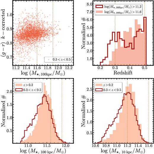
Top left: the log (M⋆, 100kpc/M⊙)–(g − r) rest-frame colour relation for the HSC massive galaxies. We k-correct the colour using the iSEDFit fitting results. Massive galaxies form a ‘red sequence’ on this figure, and there is little contamination from blue object at high-mass end. Top right: the redshift distribution of the massive galaxies. The filled and empty histograms are for the log (M⋆, 100kpc/M⊙)>11.6 and log (M⋆, 100kpc/M⊙)>11.2 galaxies. The vertical lines highlight the 0.3 ≤ z ≤ 0.5 redshift range. Bottom left: the distributions of M⋆, 100kpc of massive galaxies in this sample. Filled histogram shows the distribution for 0.3 < z < 0.5 galaxies used in this work. The empty histogram shows the distribution for the whole z > 0.2 sample as comparison. Bottom right: the distributions of M⋆, 10kpc in similar format.
In the rest of Fig. A1, we also show the distributions of redshift, M⋆, 100kpc, and M⋆, 10kpc. In this work, we focus on the massive galaxies with log (M⋆, 100kpc/M⊙)>11.6 at 0.3 < z < 0.5 where the sample is fairly complete in M⋆, 100kpc.
APPENDIX B: EXTRACTION OF 1D SURFACE BRIGHTNESS PROFILE
Here, we briefly discuss a few technical issues related to the measurements of the 1D surface brightness profiles around massive galaxies.
To derive a reliable 1D profile, it is important to mask out all the irrelevant objects around the target. At the depth of the HSC images, this becomes a challenging task, especially for massive galaxies with extended outer profiles and many satellites. At this point, the hscPipe tends to oversubtract the background around bright objects. In addition, the hscPipe deblending process performance is not optimized for extended objects. For these reasons, we perform SExtractor-like background subtraction and object detection using the SEPpython library to generate the necessary masks. Combining two different local background models and S/N thresholds, we obtain the centroid, shape, and radius that together encloses 90 per cent of flux for each object, including the one that is very close to the centre of bright galaxy (left-hand panel of Fig. A2). Based on this information, we then create the mask that covers all contaminating objects around the target after adaptively increasing the sizes of their masks according to their brightness and distance to the central target. Generally speaking, we more aggressively mask out bright objects or objects in the outskirt of the image to reduce their impact on the surface brightness profiles in the outskirt. We also create masks that are less and more aggressive than the default mask to test their impacts on the surface brightness profiles.

Left:example of the object-mask built for the Ellipse run for a typical massive galaxy in the sample. All the shaded regions are masked out. The three dashed lines (one red inner line and two blue lines) around the target at the centre outlines the three radii we defined using the flux radius of the target. We increase the mask size for objects detected in different regions separated by these apertures (which are outlined by solid, elliptical apertures with different colours) using slightly different criteria. Middle: the zoom-in intensity profile around very low intensity value (top panel), and the curve of growth of the enclosed magnitude (bottom panel) of the example galaxy. To highlight the importance of background correction, we show the profiles using both images with (red solid line) and without (black dotted line) background correction. On the top panel, besides the horizontal line that highlights the zero flux level, we also show the uncertainty of the sky background estimate using the grey-shaded region. On the bottom panel, two horizontal lines indicate the magnitudes corresponding to total flux (solid) and flux within 100 kpc (dashed). Right: compares the 1D surface brightness profiles for the same example galaxy using different masks (smaller masking region: red dashed line; larger masks: blue dashed line), or different Ellipse configurations (more aggressive pixel clipping: cyan dashed line; larger step in radius: green dashed line; using mean flux along the isophote instead of median: purple dashed line) with the default one (black solid line).
Next, we aggressively mask out all objects on the cut-out image. We then evaluate the background level using the unmasked pixels after median smoothing the masked image using box of 6 × 6 pixels.This provides estimate of global background level along with its uncertainty.Given the typical background uncertainty, the HSC WIDE image should be able to reach down to >29 mag arcsec−2 surface brightness level in the i band. However, as mentioned, we often find evidence of slightly oversubtracted backgrounds for massive galaxies in our sample. In the current hscPipe, the background on each CCD is modelled with a Chebyshev-polynomial that is fit to the smoothed image after excluding pixels with S/N > 5. This algorithm performs much better than the SDSS version (e.g. see Blanton et al. 2011), yet still oversubtracts background around bright objects and results in unphysical truncation in their surface brightness profiles.We empirically correct this issue using the background model generated by the SExtractor algorithm on the masked image (200 × 200 pixels background box size, and 6 pixels median filtering size of sky boxes). This model can account for the slightly oversubtracted background at large scale and reduce the impact from the low-surface brightness ‘wings’ of bright neighbours.We clearly see improvement in both the distributions of background pixels (more symmetric distribution; median value is closer to 0) and the surface brightness profile (middle panel of figure in Appendix B; the negative intensity and the turnover of the curve of growth in the outskirt of the ‘Original’ profile are successfully corrected) after this correction. Also, it is worth mentioning that such correction does not often affect the surface brightness profile within 100 kpc.
The procedure used to derive 1D surface brightness profile from the background-corrected, contamination-masked images is described briefly in Section 3. The uncertainties of the surface brightness profiles include the error in isophotal intensity derived by the Ellipse procedure and the uncertainty from background fluctuation estimated by the distribution of the rebinned background pixels using the above method. In practice, the profile at very low-surface brightness level is sensitive to several Ellipse configurations. After some tests, we choose to use 0.1 dex in logarithm as the step in semimajor axis length between successive ellipses, and we use the median pixel value over the elliptical annulus after rejecting outlying pixels via 3σ clipping three times. These choices are made to ensure the final μ⋆ profile is less affected by any nearby object. We also test the differences between the profiles derived using larger step, or mean value on the annulus, or fewer times of σ-clipping. Generally speaking, the surface brightness profile is very robust against these changes, especially within 100 kpc. Given our configurations, the typical photometric error is around 5 per cent level at i ∼ 26 mag arcsec−2, and is about 12 per cent down to i ∼ 28.5 mag arcsec−2. Although we want to point out that at the low surface brightness end, systematic uncertainties like background subtraction are still more important. On the right-hand panel of Fig. A2, we compare the surface brightness profiles for an example massive galaxy using different masks and Ellipse parameters. The profile within 100 kpc is very stable, and the only noticeable difference is caused by the less aggressive object mask in the outskirt.
We should also mention that we run Ellipse to allow for more sophisticated shapes than simple ellipse (fourth Fourier modes that can make isophote more ‘discy’ or ‘boxy’, e.g. Kormendy et al. 2009) to fit the isophote better. We also apply the isophotes from i-band images to other bands in a ‘force-photometry’ mode Ellipse run to get initial estimates of colour profiles.
We cannot extract reliable 1D profiles for a small fraction of massive galaxies because they are heavily masked out for either physical (e.g. late-stage major merger) or nuisance (e.g. nearby foreground galaxy or bright star) reasons. This is an intrinsic limitation of the 1D method, and it removes ∼10 per cent of the sample. We visually examine the three-colour images (gri band, like the ones shown in Fig. 1) of randomly selected galaxies with failed 1D profiles. Most of them are relatively small galaxies that are severely contaminated by nearby objects and do not affect the results of this work. Meanwhile, it is worth noting that this work does exclude most major merging systems among massive galaxies.
APPENDIX C: ESTIMATE AVERAGE M⋆/L⋆ USING ISEDFIT
In Section 4.1, we briefly explain the SED fitting procedure and the priors used. iSEDFit takes a simplified Bayesian approach. In short, it first generates a large grid of SEDs from synthetic stellar population models by drawing randomly from the prior distributions of relevant parameters (e.g. age, metallicity, dust extinction, and SFH). Based on these models, it uses the observed photometry and redshift to compute the statistical likelihood and generates the posterior PDF for each parameter. To get the best estimate of a given parameter, iSEDFit integrates the full PDF over all the other nuisance parameters. Then, the median value and the 1σ uncertainty are derived based on the marginalized PDF. Please refer to Moustakas et al. (2013) for technical details. In Fig. C1, we show an example of the iSEDFit output by visualizing the five-band HSC SED on top of the best-fitting model along with the PDF of the key parameters.
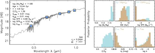
Left:example of output figure from iSEDFit that shows the SED fitting results. The open boxes show the observed fluxes in the five bands, and the solid blue dots show the best-fitting results, along with the high-resolution spectrum for this model reconstructed using the synthetic spectra from FSPS. The top left corner shows the best-fitting stellar population parameters, and the bottom right corner shows the ID, redshift of this object, and reduced χ2 of the best-fitting model. Right: the posterior distributions of a few key parameters. From top left to bottom right are: (1) stellar mass (log (M⋆/M⊙)); (2) age of the population (mass and star formation rate weighted) in Gyr; (3) star formation rate (logSFR (M⊙/yr); instant one and the one averaged over the previous 100 Myr; (4) stellar metallicity (Z/Z⊙); (5) dust extinction (AV in mag); and (6) birthrate parameter (logb; averaged over previous 100 and 1000 Myr).
Although we only use the best-fitting M⋆/L in this work, it is necessary to make sure the model is reasonable. We show the relationship between M⋆ and a few key stellar population parameters derived by iSEDFit in Fig. C2. Degeneracies among these parameters are inevitable based on only five broad-band photometry; but as expected, most massive galaxies show old stellar age, high stellar metallicity (1.5 × Z⊙ is the highest metallicity allowed by the adopted FSPS SSP models), and low dust extinction.
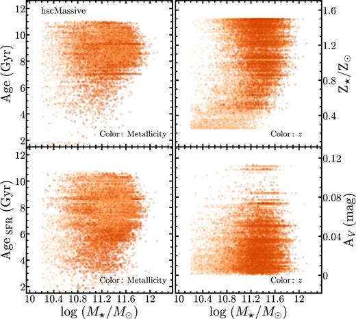
Relationships between M⋆ and key stellar population parameters from iSEDfit. The four stellar population properties are: top left: M⋆-weighted stellar population age in Gyr. Bottom left: SFR-weighted age in Gyr. Top right: M⋆-weighted stellar metallicity in unit of solar value. Bottom right: dust extinction value in V band. As expected, most of the HSC massive galaxies are old, metal-rich, and dust-free.
Meanwhile, M⋆ measurement based on SED fitting heavily depends on the adopted SSP model, the form of IMF, dust extinction law, and details in the assumption of SFH (e.g. Bernardi et al. 2017). For massive galaxies in this sample, the form of the SFH,23 and the contribution from random starburst24 rarely affect the M⋆. But the choices of SSP model, IMF, and dust extinction do systematically impact the estimates of M⋆; therefore, we look into this with a few additional tests (see Fig. C3):
Choosing the Salpeter (1955) IMF results in systematically higher M⋆ (on average +0.25 dex of log (M⋆/M⊙)) for these massive galaxies (top panel). Although there are multiple lines of evidence that favour Salpeter or an even more ‘bottom-heavy’ IMF in massive galaxies (e.g. Conroy & van Dokkum 2012; Cappellari et al. 2012), we still present the main results using Chabrier IMF to accommodate galaxies with lower M⋆ in the sample, and to be as consistent as possible with previous work. This choice of IMF does not change the main results qualitatively.
M⋆ based on the BC03 models are systematically lower than the ones based on FSPS+MILES models (middle panel). The difference shows a large scatter, and can be as large as 0.4 dex, although it is not M⋆-dependent. The BC03 results show a better average χ2 than the FSPS ones. This relates to the higher upper limit of stellar metallicity (2 × Z⊙) allowed by the BC03 model, which helps fit the shape of the SED in the red end slightly better. However, the BC03 results also show puzzlingly low stellar ages (<3–4 Gyr) for these massive, red galaxies. This could also lead to underestimated M⋆/L values. It is worth noting that both FSPS and BC03 models still have difficulties recovering SED at the very red end (between z and y bands) and reproducing the optical colour–colour relations for red-sequence galaxies (e.g. Ricciardelli et al. 2012). In this work, we decide to keep using the FSPS+MILES model as the fiducial one. Using results based on the BC03 model does not change any of our conclusions here.
On the bottom panel of Fig. C3, we compare the default model with the SED fitting results without considering the dust extinction. This choice leads to slightly smaller M⋆ values as expected. Its impact becomes slightly larger at lower M⋆ end. It does not change any of our conclusions here.
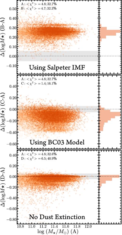
Comparisons of M⋆ estimated by iSEDFit using different model assumptions. In each panel, we plot the M⋆ from the default model against the differences with four other models: (a) default model; (b) using the Salpeter IMF instead of the Chabrier IMF (top panel); (c) using the BC03 synthetic population model instead of the FSPS one (middle panel); (d) no dust extinction (bottom panel). On each panel, the grey-shaded region highlights the typical uncertainty of the log (log (M⋆/M⊙)). For each pair of models, we highlight the median χ2 values and the fraction of galaxies with χ2 > 10.0 at the top. On each panel, we also show the histograms of the M⋆ differences on the right-hand side.
We should also point out that our methodology ignores radial variations in M⋆/L. It is well known that massive ETGs have negative optical colour gradients, indicating gradients in M⋆/L (e.g. Carollo et al. 1993; Davies et al. 1993; La Barbera et al. 2012; D'Souza et al. 2015). Assuming all massive galaxies in our sample have negative colour gradients and there is a simple monotonic relationship between optical colour and M⋆/L, the average M⋆/L we use should in principle underestimate the M⋆ in the centre, while overestimating the M⋆ in the outskirt. However, these colour gradients are shallow and they smooth out to a few times the effective radius (e.g. La Barbera et al. 2010; Tal & van Dokkum 2011; D'Souza et al. 2014, colour gradients at larger radii are not yet well quantified). Because the gradients are shallow, using an average M⋆/L is unlikely to bias our results on M⋆ measurements. In Huang et al. (2016b), the authors conduct multiband decomposition for a sample of very nearby elliptical galaxies and estimate the M⋆/L of each component separately. The sum of all components suggests a slightly higher M⋆ (0.05 − 0.10 dex when typical uncertainty of M⋆ is 0.12–0.15 dex) and the mass differences show no dependence on M⋆. Colour gradients are discussed in Section 6.3. In summary, our results about the mass dependence of μ⋆ profiles should not be affected by the assumption of a constant M⋆/L ratio because optical colour gradients in our sample do not show a dependence on stellar mass.
