


Abstract
We make use of the Survey of High-z Absorption Red and Dead Sources, an ultradeep (<26.5AB) galaxy survey that provides optical photospectra at resolution R ∼ 50, via medium-band filters (FWHM ∼ 150 Å). This data set is combined with ancillary optical and NIR fluxes to constrain the dust attenuation law in the rest-frame NUV region of star-forming galaxies within the redshift window 1.5 < z < 3. We focus on the NUV bump strength (B) and the total-to-selective extinction ratio (RV), targeting a sample of 1753 galaxies. By comparing the data with a set of population synthesis models coupled to a parametric dust attenuation law, we constrain RV and B, as well as the colour excess, E(B − V). We find a correlation between RV and B, which can be interpreted either as a result of the grain size distribution, or a variation of the dust geometry among galaxies. According to the former, small dust grains are associated with a stronger NUV bump. The latter would lead to a range of clumpiness in the distribution of dust within the interstellar medium of star-forming galaxies. The observed wide range of NUV bump strengths can lead to a systematic in the interpretation of the UV slope β typically used to characterize the dust content. In this study, we quantify these variations, concluding that the effects are Δβ ∼ 0.4.
1 INTRODUCTION
Interstellar dust is a ubiquitous component in galaxies, affecting the interpretation of photometric and spectroscopic observations (see e.g. Galliano, Galametz & Jones 2017). Made up of particles with a wide range of sizes, from 0.01 to 0.2 μm (e.g. Draine 2003), it affects light through scattering and absorption, in a wavelength-dependent manner, with increased cross-sections at shorter wavelength. Consequently, constraining the dust parameters is important to decipher the properties of the illuminating source, i.e. the stellar component. Specifically, dust corrections help derive robust star formation rates (SFRs), stellar masses, and stellar population parameters. Unfortunately, the degeneracy between dust and age complicates the derivation of robust population parameters. If the composition and distribution of dust grain sizes is known, it is possible to calculate the fraction of light lost along the line of sight. This so-called extinction curve has a fairly featureless distribution, and can be modelled by a set of power laws. In the magnitude scale, one defines the extinction in a given band, X as the magnitude increase (i.e. dimming) caused by dust in that band: AX. A parameter commonly used to characterize the dust attenuation law is the total-to-selective ratio RV = AV/E(B − V), where AV is the extinction through the V band and E(B − V) = AB–AV is the reddening, or colour excess. A high value of RV represents a grey law, where AB →AV, i.e. there is no strong wavelength dependence of the extinction law. At the other end, a low value of RV represents a very strongly wavelength-dependent law.
In addition to this general trend, there is a set of features related to specific components of the dust. In the NUV/optical region, the most prominent one is the 2175 Å NUV bump (Stecher 1969). Possible candidates to explain this feature are graphite or polycyclic aromatic hydrocarbon (PAH) molecules because this wavelength corresponds to π → π* electronic excitations in sp2-bonded carbon structures (Draine 1989) although other candidates are possible (Bradley et al. 2005). Locally, in the Milky Way and the Large Magellanic Cloud, the NUV bump is present along different lines of sight (Fitzpatrick 1999; Bekki, Hirashita & Tsujimoto 2015). Dust extinction in the Small Magellanic Cloud has been a prototypical example lacking the bump (Pei 1992). However, evidence has been recently presented to the contrary (Hagen et al. 2017). In galaxies, the interpretation of the effect of dust gets more complicated as different stellar populations are affected in different ways, so that not only dust composition but its distribution within the galaxy will have an effect on the difference between the observed spectral energy distribution (SED) and the one corresponding to a dustless case (e.g. Charlot & Fall 2000; Witt & Gordon 2000). To avoid confusion, this difference is termed attenuation, instead of extinction. Nevertheless, the overall behaviour of attenuation in galaxies is very similar to the extinction law found in stars, including the presence of the bump (see e.g. Burgarella, Buat & Iglesias-Páramo 2005; Noll et al. 2009; Conroy, Schiminovich & Blanton 2010; Wild et al. 2011; Buat et al. 2012; Hutton et al. 2014; Hutton, Ferreras & Yershov 2015; Reddy et al. 2015; Scoville et al. 2015). However, large variations are found among galaxies (Calzetti & Heckman 1999; Gordon, Smith & Clayton 1999; Johnson et al. 2007; Conroy 2010; Kriek & Conroy 2013; Zeimann et al. 2015; Battisti, Calzetti & Chary 2016). In fact, the standard dust attenuation law used in starburst galaxies lacks this bump (Calzetti et al. 2000), but the latest radiative transfer models would suggest this law would need a suppression of the carriers that produce the bump (Seon & Draine 2016). There is indeed ample evidence for PAH destruction/suppression in starbursts relative to normal star-forming galaxies, (see e.g. Wu et al. 2006; Murata et al. 2014, and references therein), see also Shivaei et al. (2017) for evidence of PAH strength variation with other galaxy properties at high redshift.
Disentangling these complex effects requires robust observational constraints of the attenuation law in star-forming galaxies. The observed variations involve the amount of dust present, grain size distribution and composition, all affected by the properties of the stellar populations such as age or metallicity (Gordon et al. 1999; Panuzzo et al. 2007; Salmon et al. 2016).
The goal of this paper is to provide new constraints on the dust attenuation law of galaxies at higher redshift exploiting the Survey of High-z Absorption Red and Dead Sources (SHARDS). SHARDS is an optimal data set for the purpose of this paper since its spectral resolution, in combination with ancillary data, probes the attenuation law in the rest-frame NUV and optical windows at redshift z ∼ 2. Furthermore, the depth of the survey allows us to study individual galaxies, avoiding stacking and its complications.
The structure of the paper is as follows: in Section 2, the data used in this study are presented. In Section 3, we describe the methodology, involving a comparison of the observed photospectra with a set of population synthesis models, including a test with simulated data. The results are discussed in Section 4, including an assessment of the effect of the observed variations in the derivation of the UV slope, β. We conclude with a summary of the results in Section 5. A standard Λ cold dark matter cosmology is adopted, with Ωm = 0.27 and H0 = 72 km s−1 Mpc−1. All magnitudes are quoted in the AB system, and stellar masses correspond to a Chabrier (2003) initial mass function (IMF).
2 SAMPLE DEFINITION
The sample is extracted from the Survey of High-z Absorption Red and Dead Sources (SHARDS; Pérez-González et al. 2013), a data set comprising deep (<26.5 AB at 4σ) optical photometry in a set of 25 medium-band filters (full width at half-maximum, FWHM ∼ 150 Å) covering a 141 arcmin2 region towards GOODS-N. SHARDS effectively provides low-resolution spectra (R ∼ 50) over the full field, without the completeness issues of standard multi-object spectroscopy. We complement the optical photometry with ACS F435W (Giavalisco et al. 2004). In addition, we use NIR fluxes from CANDELS (Koekemoer et al. 2011) in the Hubble Space Telescope (HST)/WFC3 F105W, F125W, F140W, and F160W passbands, as well as deep Ks photometry from CFHT/WIRCam (McCracken et al. 2010) and Spitzer/IRAC 3.6 μm (Fazio et al. 2004). The data are retrieved via the Rainbow1 data base (Pérez-González et al. 2008; Barro et al. 2011), using version 14.5. We select sources with a median S/N per filter of at least 5σ and with acceptable galfit models in the CANDELS WFC3/F160W images (i.e. no error flags), as well as with available photometric redshifts (however note a fraction of our sample has spectroscopic redshifts, see below). Given the flux constraint in the NUV-rest frame – mapped by SHARDS – we note that this survey is inherently biased in favour of NUV bright sources.
As the project focuses on the dust attenuation law in the rest-frame NUV + optical window, we select galaxies over a redshift interval such that the NUV bump is included within the spectral range of SHARDS (0.5–0.9 μm). The sample comprises 1807 galaxies at 1.5 < z < 3, with a median redshift of 2.14. We note that 16.7 per cent of the sample has available spectroscopic redshifts. This subsample of 302 galaxies has a photo-z accuracy of 0.4 per cent given by the median of the distribution |Δz|/(1 + z), mostly thanks to the photospectra provided by the medium-band filters (Pérez-González et al. 2013; Ferreras et al. 2014). There is no significant trend between the photometric redshift accuracy and the apparent magnitude of the sources (between F160W = 22 and 25 AB). The number of catastrophic failures – defined as those photometric redshifts with an accuracy outside of three times the rms of the distribution – is 3.9 per cent. The above criteria favour bright UV sources, therefore, we need to check whether the photospectra are contaminated by AGN light. We cross-match our sample with the X-ray sources in the 2 Ms Chandra Deep Field North (Alexander et al. 2003), following Trouille et al. (2008) to convert fluxes in the 2–8 keV band into luminosities. Only 33 sources have an X-ray detection, with an average 〈LX〉 = 2.9 × 1043 erg s−1, and only two sources brighter than LX > 1044 erg s−1. Nevertheless, we discard all those sources with an X-ray detection, to make sure our data are dominated by stellar light. Moreover, we discard potential sources with an obscured AGN, following the criterion of Donley et al. (2012) based on flux ratios from Spitzer/IRAC. Our final sample therefore comprises 1753 star-forming galaxies. Note that one of the adopted selection criteria requires a good surface brightness fit in F160W, mapping a rest-frame interval between B and R bands. Furthermore, the distribution of the Sérsic index from the CANDELS surface brightness fits in the WFC3/F160W band (see Section 4) is rather low, suggesting a negligible contribution from a central AGN.
Fig. 1 shows the sample with respect to the SFR, following Rujopakarn et al. (2013). In this study, the authors estimate SFR based on single band measurements with Spitzer/MIPS at 24 μm, out to z < 2.8 (see section 5 of that reference for details).
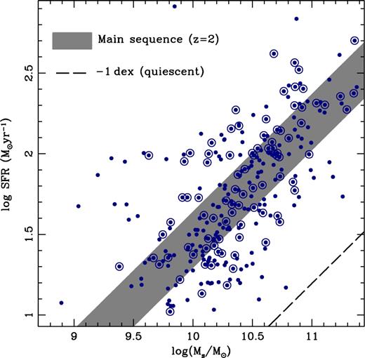
Correlation between SFR and stellar mass. Only those sources with available 24 μm fluxes are shown (blue dots). For reference, the main sequence at z = 2 is shown, as defined by Speagle et al. (2014, grey shaded region). The dashed line is an offset of the above by −1 dex to guide the eye towards the region where quiescent galaxies should lie. Single dots represent galaxies with a photometric redshift; whereas those encircled by an outer ring are galaxies with a spectroscopic redshift. The figure does not include sources only with an upper limit estimate to the SFR.
Note we only show in the figure those galaxies with an observed 24 μm flux, avoiding here galaxies with just an upper bound to the SFR. For reference, the main sequence at z = 2 (as derived by Speagle et al. 2014) is shown as a grey shaded region that includes the observational scatter in the relation. This redshift is approximately the median value of our sample. The dashed line represents the loci of quiescent galaxies by offsetting the main-sequence relation by −1 dex in SFR. This figure shows that our sample lies mainly around the main sequence (grey shaded area) and covers a wide range of stellar mass. We also note that the sample does not feature any significant selection bias between mass and redshift.
We follow the prescription proposed by Conroy et al. (2010, CSB10), defined by two parameters, namely the NUV bump strength (B) and the total-to-selective extinction ratio (RV).
3 CONSTRAINING THE DUST ATTENUATION LAW
Following the aforementioned CSB10 dust attenuation law at the fiducial value B=1, RV=3.1, this parametrization recovers the standard Milky Way extinction law of Cardelli, Clayton & Mathis (1989). A third parameter controls the net amount of reddening, and can be described either by the attenuation in a reference band (e.g. AV) or by a colour excess [e.g. E(B − V)]. We adopt the latter.
Fig. 2 shows the transmission curves of the 32 filters used in this study, including the HST/ACS B band, 25 SHARDS filters, the NIR HST/WFC3 passbands from CANDELS, CFHT/WIRCam Ks, and Spitzer/IRAC 3.6 μm. This set spans a wide enough spectral range to constrain the dust-related parameters. The SHARDS fluxes provide a good sampling of the region around the NUV bump over the selected redshift range. For reference, the figure includes the Calzetti et al. (2000) law (thin line), the standard Milky Way extinction (thick line), and an additional case from CSB10 (dashed line), adopting a weaker bump (B=0.5) and a steeper wavelength dependence (RV=2). This paper does not aim at exploring the distribution of dust within galaxies. Therefore, we only consider the effect of dust as a foreground screen acting on the underlying stellar light. Such a simplified model gives a robust constraint on the attenuation law. The only difference between the assumption of a foreground screen or a homogeneous distribution of dust and stars is in the apparent optical depth. The drawback is, of course, the inability to disentangle dust properties from dust-star geometry in the interpretation of the results. Our aim is, therefore, to use the observed fluxes to constrain the attenuation law, which requires marginalizing over the parameters that control the illumination source (i.e. the stellar populations). We use the stellar population synthesis models of Bruzual & Charlot (2003, hereafter BC03), with the standard assumption of a Chabrier (2003) IMF. The adopted range of parameters can be found in Table 1.
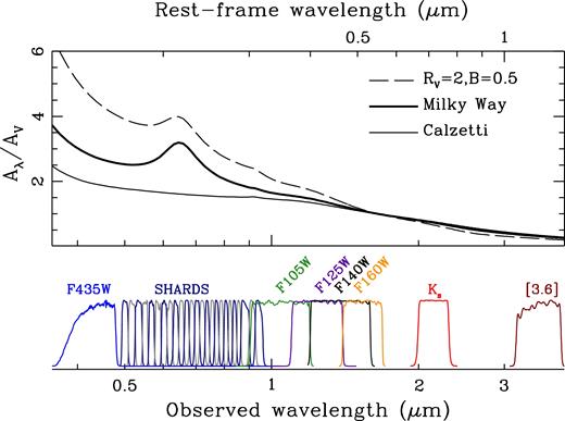
The set of filters used in this analysis is shown as a function of observed (bottom) and rest-frame wavelength (top), with the latter assuming a galaxy at z = 2, roughly corresponding to the median redshift of the sample. The transmission curves are normalized at the peak value. The top panel shows three choices of the attenuation law, as labelled. Note the SHARDS medium-band filters sample the region around the NUV 2175 Å bump at the redshifts of interest (1.5 < z < 3).
Parameter range of the grid of models (see the text for details).
| Observable | Parameter | Range | Steps |
|---|---|---|---|
| Age (log scale) | log (t/Gyr) | [−2, +0.6] | 16 |
| Metallicity (log scale) | log (Z/Z⊙) | [−2, 0.3] | 8 |
| Colour excess | E(B − V) | [0, 1.5] | 24 |
| Total-to-selective extinction ratio | RV | [0.5, 5] | 24 |
| NUV bump strength | B | [0, 1.5] | 24 |
| Number of models | 1769 472 |
Our methodology entails a comparison between a large grid of BC03 models and the observations. The grid assumes simple stellar populations (SSPs), corresponding to a single age and metallicity. We define a large set of lookup tables of model photometry to be used with all galaxies. Therefore, redshift is an additional parameter in the grid. An important issue to bear in mind is that the response profile of the medium-band filters of the SHARDS survey depends on the position of the source on the focal plane (Pérez-González et al. 2013). The net effect is a position-dependent shift of the transmission curve in wavelength, and this shift can be as large as the extent (FWHM) of the passband (see Pérez-González et al. 2013; Cava et al. 2015). Therefore, each source effectively sees an independent set of SHARDS filters, in principle requiring an individual grid of model fluxes accounting for those filter offsets, prohibitively expensive in computing time. However, this effect can be modelled accurately by a linear fit of the model fluxes to the central wavelength of each filter. Since the 2175 Å bump is the only remarkable spectral feature in the range covered by SHARDS at these redshifts, and it is much wider than the FWHM of the filters, a simple linear parametrization of the effect of these shifts on the photometry gives accurate results, with residuals well below the flux uncertainties. We implement this approximation for each of the 25 SHARDS filters by measuring the model fluxes shifted by ±100 Å with respect to the central wavelength, in order to create two different sets of grids from which we define the linear interpolation. Regarding redshift, we create one set of grids at intervals Δz=0.1 between z=1.5 and 3. For each galaxy, we apply a linear interpolation between the reference redshift values from the grid that straddle the observed redshift.
Fig. 3 illustrates the typical fitting results for three galaxies at Ks ∼ 22–23 AB, where the observed fluxes are plotted in red, and the best-fitting model as a solid black line. The figure is split left/right between the optical and the NIR windows. We include the FWHM of the NIR passbands as horizontal error bars, and show the best fit at a higher spectral resolution than the one used in the (photometric) analysis to show the type of stellar populations typically found in our sample, with SSP-equivalent ages between 10 Myr and 1 Gyr (see the inset in Fig. 5). Each galaxy is labelled by their SHARDS ID, redshift and magnitude in the Ks band, and the best fit to the dust parameters B and RV is also shown. In general, the whole sample produces good fits, with an average, reduced |$\langle \chi ^2_r\rangle = 1.54$| (considering 32 fluxes and five free parameters). The blue dotted lines represent the best-fitting case when enforcing a Calzetti et al. (2000) attenuation. Note in all cases the fit is significantly worse for this choice of attenuation. Note the prominent NUV bump in the SHARDS photometry of galaxy SH09310 at 0.75 μm in the middle-left panel, for which a Calzetti law cannot give a good fit.
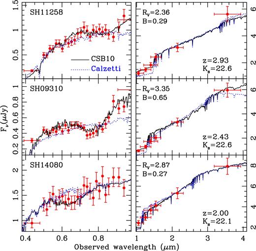
Example of the fits to the observed fluxes in three galaxies, labelled by their SHARDS ID, redshift, and Ks AB magnitude, as well as the best-fitting values of B and RV. The red dots are the observed fluxes, shown with their flux uncertainties. The solid line is the best fit to the models, shown at a better resolution than the photometric data to illustrate the type of populations being considered. For reference, the best-fitting model, restricting the analysis to a Calzetti law, is shown as a dotted line. The wavelength coverage is split between the observed frame optical (left) and NIR (right). Note the prominent NUV bump in SH09310 (middle-left panel), mapped at 0.75 μm at the redshift of the galaxy.
There are two main issues that need to be assessed regarding the methodology: (1) How well does the grid-based method behave with respect to the linear interpolations performed both in redshift and within the transmission curve of each of the 25 SHARDS filters? (2) We approximate the illumination source as an SSP. How well can this treatment reproduce the complex populations typically found in galaxies? These can be addressed by running a set of simulations, comparing the input values of the dust attenuation law with the retrieved values following this methodology. We create five sets of mock data, each corresponding to a different parametrization of the star formation history (SFH): an SSP, representing single burst galaxies; a two-burst model (2SSP) that overlays a young component over an older one, an exponentially decaying rate (EXP), an exponentially increasing rate (EXPP), and a constant star formation rate followed by a truncation (CST). These sets of synthetic data represent the typical range of potential formation histories explored in the literature (e.g. Papovich et al. 2011; Ferreras et al. 2012; Reddy et al. 2012; Domínguez Sánchez et al. 2016). In all cases, the illumination source derived from the mixture of stellar populations is subject to a single foreground screen with parameters B, RV, and E(B − V). Each of the five sets comprise the same number of galaxies as the original sample, with the same redshift distribution and photometric uncertainties. For each simulated galaxy, we draw a random estimate for each of the parameters that define the sample (see Hutton et al. 2015, for details), therefore we assume the mock sample has uncorrelated dust parameters. This is a property we exploit below to assess potential systematics.
The difference between the true input values and those retrieved from the SSP grid-based analysis is presented in Fig. 4, for the five different choices of SFH. The mock data explore a wide range of the age distribution, metallicity, and dust. These figures show the comparison between the input and the retrieved values. Even though the actual SFHs of galaxies are more complex than the SSP-adopted set in our grids, this exercise illustrates how well one can recover the attenuation parameters by marginalizing over a large grid of SSPs. A similar result, although based on a different set of photometric filters, was found by Hutton et al. (2015). The simulations can also be used to calibrate the methods, by performing a linear fit between the input and the output parameters. We note that this calibration step is not essential, but it helps to increase the accuracy in the determination of the dust-related parameters. Table 2 shows the calibration fits. In order to avoid the effect of outliers, the fits are obtained after clipping the sample at the 3σ level. The table also shows the rms scatter of the comparison between the input value and the retrieved value, which serves as an estimate of the accuracy of the method, namely ΔB=0.18; ΔRV=0.75, and ΔE(B − V) = 0.10 mag.
![We illustrate the accuracy of the method in constraining the dust attenuation parameters by comparing input and retrieved values in a set of simulations [ΔRV, ΔB, and ΔE(B − V)]. Five sets of SFHs are considered, from top to bottom: constant star formation rate (CST); exponentially increasing star formation rate (EXPP); exponentially decaying star formation rate (EXP); a superposition of two simple stellar populations (2SSP) and a simple stellar population (SSP). The width of the distributions provide an estimate of the uncertainties expected in the analysis (see column 4 in Table 2).](https://oup.silverchair-cdn.com/oup/backfile/Content_public/Journal/mnras/475/2/10.1093_mnras_stx3334/1/m_stx3334fig4.jpeg?Expires=1750237342&Signature=s8SotF626gE-TmS65HT3SRDmevjk-d6RK-XGKOW8sNHDY-YN3NGAvCeNkVxF96UjTWuxC0NZtWhp6I5~LKKrAFBM656Wgl67vAqMvB0RRRHKBFFpewduEERq9fLdBYuDhHwuUs1M1kPfgbe82OQ9q~Gplg21CROlVlRmXRrsZdCBtO-3X5DXinWNxgWImnRM48CPRwUyqXNvhD1FU5-WXKBnbu1sSzGKwar2K54kA1M90FRn2b~lN2N-kprcmQzwkq9Eph2dThtPF305WZ3QygNs2QJTH0je3yZRvnjZxmuvMrSYntuzctX1E836xEEk3UDBU8LtGDK3zahZDANUgA__&Key-Pair-Id=APKAIE5G5CRDK6RD3PGA)
We illustrate the accuracy of the method in constraining the dust attenuation parameters by comparing input and retrieved values in a set of simulations [ΔRV, ΔB, and ΔE(B − V)]. Five sets of SFHs are considered, from top to bottom: constant star formation rate (CST); exponentially increasing star formation rate (EXPP); exponentially decaying star formation rate (EXP); a superposition of two simple stellar populations (2SSP) and a simple stellar population (SSP). The width of the distributions provide an estimate of the uncertainties expected in the analysis (see column 4 in Table 2).
Corrections to the data: πtrue = απOBS + β. Derived from simulations shown in Fig. 4. Column 1 identifies the dust attenuation parameter, Columns 2 and 3 are the best linear fit parameters taking all simulated SFHs into account. Column 4 is the rms scatter of the difference between true and extracted values.
| π | α | β | rms(Δπ) |
|---|---|---|---|
| RV | 1.0329 | −0.337 | 0.72 |
| B | 0.9772 | +0.073 | 0.18 |
| E(B − V) | 0.7738 | +0.032 | 0.07 |
| π | α | β | rms(Δπ) |
|---|---|---|---|
| RV | 1.0329 | −0.337 | 0.72 |
| B | 0.9772 | +0.073 | 0.18 |
| E(B − V) | 0.7738 | +0.032 | 0.07 |
3.1 Effect of nebular emission
The most significant contribution from nebular emission is in relatively narrow spectral lines. Our methodology removes outliers to the fits at specific wavelengths, so we are resilient to such contamination. However, an additional contribution that can affect the flux measured in all passbands is from the nebular continuum. Since emission from the nebular continuum is not included in BC03 models, we explore the impact of that effect in our method using a set of SSPs from the starburst 99 models (Leitherer et al. 1999). We assume solar metallicity and a Salpeter IMF for practicality, and compare this relative change for three choices of the age: 10 Myr (solid blue), 30 Myr (short dashed orange), and 50 Myr (long dashed red), within the spectral range used here. Fig. 5 justifies our approximation by comparing the relative flux increase contributed by nebular emission. We show three cases corresponding to young populations from the STARBURST99 models (Leitherer et al. 1999), adopting a constant SFH, Salpeter IMF, and solar metallicity. Even at the youngest ages (∼10 Myr), the contribution from the nebular continuum stays below the ∼0.5 per cent level. For reference, the inset in Fig. 5 shows the retrieved SSP ages from the sample with respect to stellar mass. Note that the majority (∼81 per cent) of our sources have SSP ages older than 30 Myr. Since an uncorrected SSP age should be younger if nebular emission is not accounted for, we conclude that this component is not essential in our analysis.
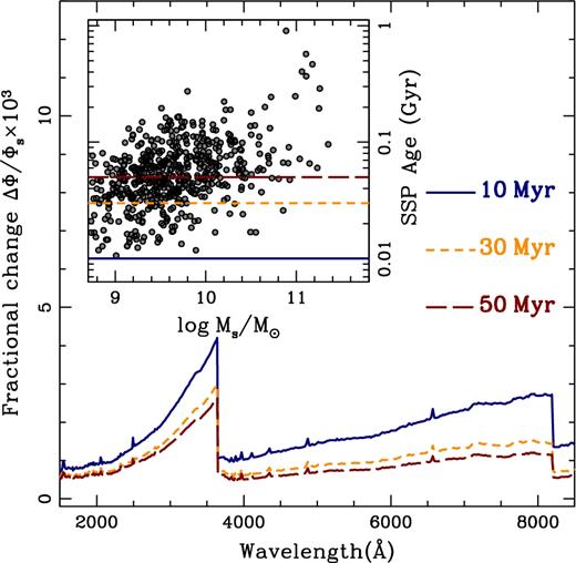
Relative change in the flux contributed by nebular continuum emission at three different ages, following the starburst 99 models (Leitherer et al. 1999) at solar metallicity, for a continuous SFH with a Salpeter IMF. The inset shows the derived SSP equivalent ages of our sample, following the same colour coding of the three choices of SSP age. To avoid overcrowding the plot, only one out of three data points (randomly chosen) are shown.
4 DISCUSSION
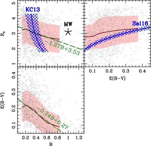
Correlations between dust attenuation parameters. Individual data points are shown as grey dots, whereas the thick solid line and shading represent a moving median and rms scatter, respectively. The star in the top-left panel (labelled MW) corresponds to the standard extinction law in the Milky Way, and the blue hatched region mark the estimates from Kriek & Conroy (2013, labelled KC13). The top-right panel shows, also in blue, the trend presented in Salmon et al. (2016, labelled Sal16). These two comparisons required the conversion from their attenuation slope δ to a standard RV (see Appendix A for details). We also present a simple linear fit to the correlations on the left-hand panels (green dashed lines), described by equations (2) and (3). Note we do not attempt such a fit between RV and E(B − V) because there is a large scatter of the data points. In Kriek & Conroy (2013), both sSFR and stellar mass are derived galaxy properties, with the equivalent width of H α used as an SFR proxy.
The top-right panel compares RV and E(B − V), showing an overall wide range of values. Although the running median suggests an increase of RV with colour excess, we decide not to quote any linear fit given the large scatter found in the individual data points. Salmon et al. (2016) also relate the total-to-selective ratio and reddening with δ and Eb, finding that galaxies with a higher dust content obey a flatter attenuation curve (i.e. higher RV), qualitatively following the trend of our running median, as shown by the blue hatched region in the top-right panel – a similar conversion from δ to RV was performed, following a least squares fit (Appendix A). We note that our results qualitatively follow the prediction of Chevallard et al. (2013), who suggest a trend towards a steeper (i.e. lower RV) attenuation law at lower opacities, i.e. lower E(B − V). However, the scatter in our results is too large to derive any trend between these two parameters.
The observed trend between RV and B could have two possible origins. First, we may assume that the observed variations are due to changes in the composition of the dust. In this case, we would expect that very small dust particles are responsible for the bump, as commonly accepted (e.g. Draine 1989). Small grains will produce a steeper attenuation law, closer to Rayleigh scattering, therefore leading to low values of RV, and – according to the observations – to a strong NUV bump. Alternatively, different dust geometries may play an important part, due to the fact that the attenuation law can be age-dependent within the complex distribution of stellar populations in galaxies. Radiative transfer models show that a patchier distribution of dust within the galaxy will produce both a weaker bump and a greyer (i.e. higher RV) attenuation (e.g. Charlot & Fall 2000; Witt & Gordon 2000; Panuzzo et al. 2007). Therefore, the observed correlation, described by equation (2), could be interpreted as a trend with respect to the clumpiness of the dust distribution. We also find that a stronger bump is found at lower reddening. Note that the colour excess stays below 0.5 mag. This is possibly due to a selection bias since dustier galaxies would appear fainter than the flux limit of the SHARDS survey.
The relation between the dust-related parameters and general galaxy properties is presented in Fig. 7, showing, from left to right, redshift, the Sérsic index of the CANDELS surface brightness fits in the WFC3/F160W band, its corresponding effective radius (in kpc, physical units) and axis ratio (q), the stellar mass (in units of M⊙), SFR (in M⊙ yr−1), and specific star formation rate (sSFR, in yr−1). The lines follow a running median, split with respect to stellar age, with red-dashed (blue-solid) representing the oldest (youngest) tercile of the age distribution. The shaded regions mark the error in the median. In general, there are no strong trends with these parameters, except for a consistent split with respect to stellar age. Note the steeper trend for the older population with respect to stellar mass (i.e. an increasing dust content, with a weaker bump in more massive galaxies), mirrored in the trend with respect to sSFR. This correlation is not unexpected (e.g. Zahid et al. 2013), since dust is a component associated with the presence of star-forming gas. Regarding differences with respect to stellar age, the largest offset is found with respect to RV. For instance, at fixed stellar mass, older galaxies will have greyer extinction (i.e. higher RV). No significant correlation is found between the NUV bump strength and most of the parameters shown in Fig. 7, although the younger populations consistently feature slightly weaker bumps (cf. Wild et al. 2011; Kriek & Conroy 2013). For reference, Table 3 lists the correlation between the stellar mass and the dust-related parameters.
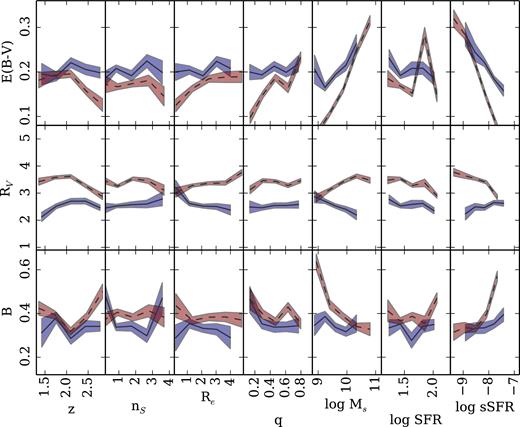
Relation between the dust-related parameters of the dust attenuation law (from top to bottom: colour excess, total-to-selective ratio, and NUV bump strength) and several observables, from left to right: spectroscopic redshift, Sérsic index, semimajor axis in physical units (kpc) – measured in the WFC3/F160W band, axis ratio, stellar mass (in M⊙), SFR (in M⊙ yr−1), and sSFR (in yr−1). In all panels, the lines (and shade) trace the median (and 1σ error) of subsamples, split with respect to stellar age (blue-solid: young tercile, red-dashed: old tercile). The median stellar age of the distribution is 5.2 Myr. From the plots displayed above, we observe that the most significant correlation is seen between the sSFR and two of the dust parameters, the colour excess and NUV bump strength. In particular, they both exhibit opposite trends. An increment in sSFR correlates with a decrease in colour excess and is associated with a stronger NUV bump strength. Furthermore, the trend of the dust-related parameters with stellar mass is shown in Table 3.
Correlation between stellar mass and dust-related parameters, as shown in Fig. 7. Each column gives the median value and the rms scatter per bin in stellar mass. The results are shown for the younger and older terciles of the distribution. The last column (n) gives the number of data points per bin.
| log Ms/M⊙ | E(B − V) | RV | B | n |
|---|---|---|---|---|
| YOUNG (tSSP ≳ 4.1 Myr) | ||||
| 8.69–9.06 | 0.21±0.15 | 2.86±1.03 | 0.35±0.22 | 24 |
| 9.06–9.42 | 0.17±0.10 | 2.70±1.08 | 0.39±0.30 | 179 |
| 9.42–9.78 | 0.19±0.09 | 2.52±0.93 | 0.34±0.23 | 138 |
| 9.78–10.15 | 0.21±0.10 | 2.40±0.86 | 0.32±0.17 | 71 |
| 10.15–10.51 | 0.26±0.11 | 2.20±0.95 | 0.35±0.21 | 31 |
| OLD (tSSP ≳ 6.7 Myr) | ||||
| 8.70–9.17 | 0.06±0.05 | 2.81±0.72 | 0.64±0.19 | 30 |
| 9.17–9.63 | 0.11±0.06 | 3.12±0.77 | 0.44±0.25 | 162 |
| 9.63–10.10 | 0.16±0.08 | 3.41±0.80 | 0.39±0.22 | 193 |
| 10.10–10.57 | 0.25±0.07 | 3.63±0.73 | 0.34±0.16 | 105 |
| 10.57–11.04 | 0.32±0.09 | 3.47±0.80 | 0.33±0.23 | 62 |
Note the method is potentially degenerate between RV and age: a steep, i.e. lower RV will remove more UV/blue photons, an effect that is mimicked by changing the age to older values. Therefore, the potential systematic goes in the opposite direction, strengthening the observed result as an intrinsic trend. In addition, metallicity may also contribute to this degeneracy, but the observational constraint on metallicity with the available data is very poor.
4.1 Variations in the attenuation law and the NUV slope
The results presented above show a significant variation of the dust attenuation parameters among galaxies (Fig. 6). We consider now the effect of this variation on the derivation of the UV power-law index, β, used as a standard proxy of dust content in galaxy spectra. Although the standard definition of β (Calzetti, Kinney & Storchi-Bergmann 1994) purposefully avoids a region close to the NUV bump, this feature is rather broad, so it is important to assess the effect of these variations. Moreover, since the NUV bump strength appears to be correlated with other galaxy properties, one could expect a systematic bias in the measurement of β.
In order to quantify this effect, we construct a set of synthetic populations – from the BC03 models – subjecting them to various levels of dust attenuation. Fig. 8 shows an example for a 5 Myr SSP at solar metallicity, affected by a range of attenuation laws. We compare the extracted β between a standard Calzetti et al. (2000) law and a generic CSB10 law for several choices of RV (as labelled).
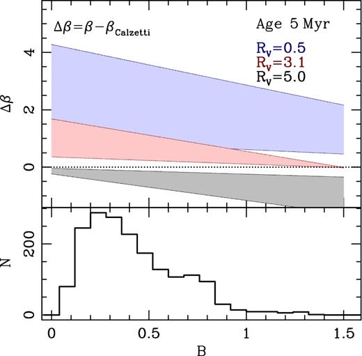
Top: estimate from a synthetic population of the difference (Δβ) between the UV-continuum slope adopting a CSB10 dust parametrization and a Calzetti law (RV = 4.05 and B=0). The model assumes a 5 Myr population with solar metallicity, and explores a range of bump strength values (B, horizontal axis). The dotted line indicates Δβ = 0. The different shaded regions represent three choices of RV, from top to bottom {0.5,3.1,5.0} , each region ranges between E(B − V)=0.1 and 0.5 mag. Bottom: distribution of the observed NUV bump strength parameters in our SHARDS sample.
The slope β is derived following the standard procedure, fitting a power law to the flux in the NUV region F(λ) ∝ λβ, over the 1300–2600 Å spectral window defined in Calzetti et al. (1994).
We define Δβ as the difference between the value from the CSB10 attenuation case, and the standard (i.e. Calzetti) choice, for the same stellar population parameters and with the same colour excess E(B − V). We consider a range of NUV bump strengths as given by the horizontal axis. The bottom panel shows the actual distribution of best-fitting B from the SHARDS data set. The shaded areas in the top panel extend over a [0.1–0.5] mag range of colour excess, E(B − V). We note that if we choose as reference the standard Milky Way extinction law (Cardelli et al. 1989), the results do not change appreciably. A robust determination of UV slope is only possible with young populations ( ≳ 200 Myr), where the spectrum in the UV region is well fitted by a power law. The chosen stellar age, or metallicity, does not affect Δβ, as long as the population is young enough (i.e. within the aforementioned range).
Fig. 8 shows that the UV slope correction can potentially lie in the range Δβ ∈ [−1, 4], depending on the dust-related parameters. To assess the effect of the variation in dust attenuation properties among star-forming galaxies, we decided to estimate the UV slope for the SHARDS sample (βobs), and to correct it to a common reference – adopting the Calzetti et al. (2000) law – by taking into account the constraints on the attenuation parameters, on a galaxy-by-galaxy basis. Therefore, we define a corrected UV slope: βc ≡ βobs − Δβ. Quantitative estimates on the effects of variations in the NUV bump and RV on β have been discussed previously (see e.g. Buat et al. 2011, 2012; Reddy et al. 2015).
We obtained the slope following the procedure mentioned above, using the SHARDS photometric measurements corresponding to filters that fall within the intervals proposed in Calzetti et al. (1994). The correction, Δβ, is obtained for each galaxy with synthetic data equivalent to Fig. 8, but adopting the corresponding best-fitting values of the population and dust parameters, leading to a corrected (i.e. Calzetti-equivalent) βc. Fig. 9 shows the difference between the distribution of original (orange dashed line) and corrected UV slopes (red solid line). This comparison shows that although the changes could be, in principle, rather high, as shown in Fig. 8, the actual properties of the galaxies lead to changes Δβ ∼ 0.4. The arrows in Fig. 9 give the position of the median distribution in raw and corrected β.
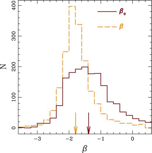
Histogram of the distribution of the original measurements of the UV slope, β, from the SHARDS data (orange dashed line) and the corrected slope, βc (red solid line, see Fig. 8 and the text for details). The arrows mark the median of both distributions.
Figs 10 and 11 show the distribution of βc with respect to several observables of our SHARDS sample. In both figures, the sample is split with respect to age, showing the median (lines) and median error (shaded regions) of the youngest (oldest) tercile in stellar age shown in blue-solid (red-dashed). Fig. 10 shows the relation of UV slope with stellar mass, with a weak positive correlation in both subsamples. We include in this figure histograms of the two parameters plotted, following the same colour coding. The mass histogram (top) shows a mass-age trend. This is not unexpected, as both stellar metallicity and age correlate with stellar mass (see e.g. Gallazzi et al. 2005). The βc histogram to the right of Fig. 10 reflects the wider scatter in UV slope of the younger subset, but intriguingly, the youngest population shows the flattest UV slopes, indicative of a higher contribution from dust.
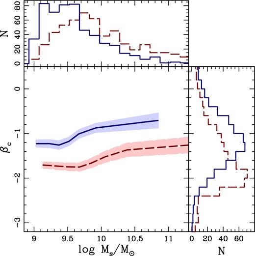
The corrected UV slope βc is plotted as a function of the stellar mass. Histograms for these two parameters are shown in the top/right panels. In the central plot, the blue-solid (red-dashed) lines represent objects with ages in the first (third) tercile of the age distribution, therefore, blue (red) represents younger (older) populations. The solid lines and shaded regions show the mean, and its uncertainty, respectively. In the histograms, the blue (red) lines are also segregated with respect to young (old) ages, taking the lowest (highest) tercile.
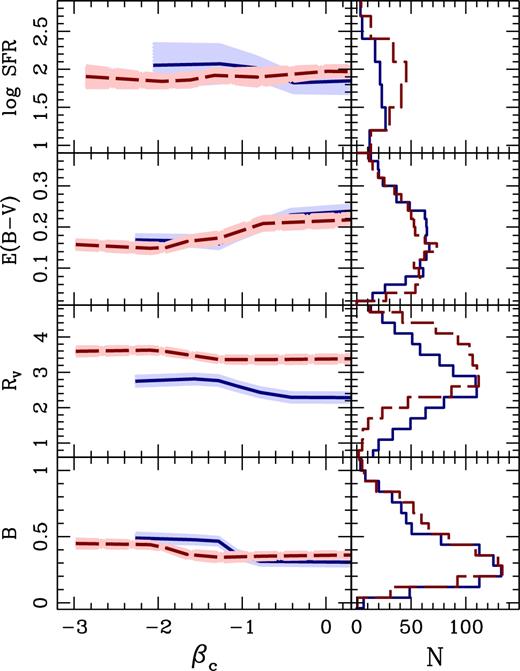
The corrected NUV slope, βc, is shown against the star formation rate (top) and the dust-related parameters; second panel from the top, downwards: colour excess, total-to-selective extinction and NUV bump strength. The line and colour coding follow the notation in Fig. 10, split with respect to age, with red-dashed (blue-solid) representing old (young) populations. The panels on the right show the distribution of the best-fitting parameters.
Fig. 11 shows the distribution of βc with respect to the dust-related parameters. A significant trend is found between colour excess or bump strength and βc, where galaxies with a shallower UV slope are dustier, and feature weaker bumps. The trend with colour excess is known for local starbursts (Calzetti et al. 1994). When split with respect to age, it is worth mentioning the trend in RV, where at fixed βc, older galaxies have higher RV (i.e. greyer laws). This trend is also evident in the histograms to the right of Fig. 11.
Finally, it is important to note that SSP age, dust content (quantified through the colour excess), and RV will induce changes in the observed UV slope, since changes in these parameters will affect the shape of the spectral continuum in similar ways. However, our simulations (Section 3) showed that E(B − V) and RV can be retrieved irrespective of this degeneracy.
5 SUMMARY
Taking advantage of the SHARDS, we constrain the dust attenuation law in a sample of star-forming galaxies over the redshift range 1.5<z<3. SHARDS is an ultradeep (<26.5 AB, at 4σ) galaxy survey covering 141 arcmin2 towards the GOODS North field that provides optical photospectra at resolution R∼50, via medium-band filters (FWHM∼150 Å). Our sample, selected to have high enough signal in the rest-frame NUV region, comprises 1753 galaxies, covering a stellar mass range 9 ≳ log M/M⊙ ≳ 11. We apply a Bayesian method that explores a wide range of stellar population and dust attenuation properties. The latter follows the functional form proposed by CSB10, and is defined by two parameters: the total-to-selective extinction ratio (RV), and the NUV bump strength (B), along with a normalization factor, where we use the colour excess, E(B − V). A comparison with synthetic models suggests an accuracy ΔE(B − V)=0.07; ΔB=0.18; and ΔRV=0.72 (rms), without any significant systematic correlation among the extracted parameters. Furthermore, the comparison with synthetic models shows that the retrieved values of B, RV, and E(B − V) are largely independent of the parametrization of the SFH.
The observational constraints reveal a wide range of values in B and RV, suggesting complex variations both in the geometric distribution of dust within galaxies, and/or in the chemical composition of the dust. A comparison between parameters (Fig. 6) shows significant correlations between RV, B, and E(B − V), towards a steeper attenuation (smaller RV) with increasing B, and a stronger NUV bump with decreasing colour excess, quantified by the linear fits shown in equations (2) and (3). This result qualitatively agrees with the study of Kriek & Conroy (2013), although our results probe a wider range in B and RV, and we note that our analysis is done on individual galaxies, thanks to the depth of the SHARDS data set. As expected, we find a trend between colour excess and stellar mass, and most notably between SSP-equivalent age and RV, so that the older populations feature a greyer attenuation (Fig. 7). We emphasize that the simulations, including a wide range of SFHs, show that the methodology does not introduce any spurious covariance between these parameters.
We also explored the possibility that the observed wide range of attenuation parameters could affect the interpretation of the UV slope. The presence of the NUV bump is especially relevant, since β is measured in a nearby spectral window. Although tests with simulated data reveal potentially large changes in β due to the NUV bump, we conclude from the observations that realistic corrections can be of the order of Δβ ∼ 0.4. The UV slope is found to correlate with the age and the stellar mass of the galaxy (Fig. 10). Moreover, at fixed UV slope, older galaxies feature a higher RV, a consistent trend found throughout this study. Although the interpretation of variations in the attenuation law can be related to either the composition or the geometric distribution of dust compared to other stars within the galaxy, this trend with respect to age suggests dust geometry changes as the main cause, leading us to propose that the relation between RV and B shown in the top-left panel of Fig. 6 (equation 2) is caused by variations of clumpiness in the distribution of dust within star-forming galaxies. We will follow up this suggestion in a future paper, aimed at breaking the degeneracy between dust composition and distribution in galaxies, and combining these results with MIR and FIR data.
Acknowledgements
We would like to thank Sandro Bressan for his comments and suggestions. MT acknowledges support from the Mexican ‘Consejo Nacional de Ciencia y Tecnología’ (CONACyT), with scholarship #329741, as well as the Royal Astronomical Society for travel funding related to this project. EMQ acknowledges the support of the European Research Council via the award of a Consolidator Grant (PI McLure). PGP wishes to acknowledge support from Spanish Government MINECO Grants AYA2015-63650-P and AYA2015-70815-ERC. This work has made use of the Rainbow Cosmological Surveys Database, which is operated by the Universidad Complutense de Madrid (UCM), partnered with the University of California Observatories at Santa Cruz (UCO/Lick, UCSC). Based on observations made with the GTC, installed at the Spanish Observatorio del Roque de los Muchachos of the Instituto de Astrofísica de Canarias, in the island of La Palma.
Footnotes
REFERENCES
APPENDIX A: RELATION BETWEEN δ, Eb AND RV, B
We translate the dust parameters δ and Eb used in the definition of the attenuation law in Kriek & Conroy (2013), into RV and B by use of a python script. The script fits one parametrization (δ,Eb) into the other one (RV, B), within the spectral window 1700–6000 Å. Figs A1 and A2 show the relation between these two sets of dust parameters (solid red line).

Relation between B and Eb for three choices of δ, as labelled. The linear fits to these trends are shown in equation (A1).
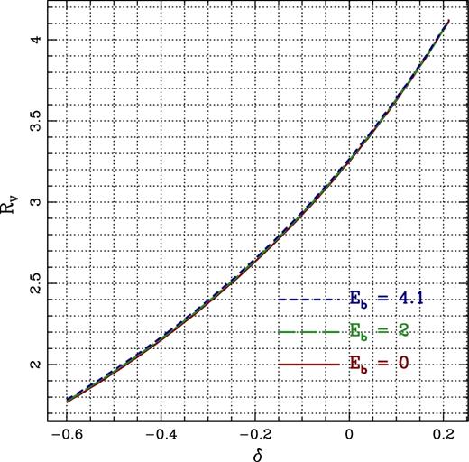
Relation between RV and δ for three choices of the NUV bump strength parameter Eb, as labelled. The quadratic fit to this trend (regardless of Eb) is shown in equation (A2).
