


Abstract
Line emission is strongly dependent on the local environmental conditions in which the emitting tracers reside. In this work, we focus on modelling the CO emission from simulated giant molecular clouds (GMCs), and study the variations in the resulting line ratios arising from the emission from the J = 1–0, J = 2–1, and J = 3–2 transitions. We perform a set of smoothed particle hydrodynamics simulations with time-dependent chemistry, in which environmental conditions – including total cloud mass, density, size, velocity dispersion, metallicity, interstellar radiation field (ISRF), and the cosmic ray ionization rate (CRIR) – were systematically varied. The simulations were then post-processed using radiative transfer to produce synthetic emission maps in the three transitions quoted above. We find that the cloud-averaged values of the line ratios can vary by up to ±0.3 dex, triggered by changes in the environmental conditions. Changes in the ISRF and/or in the CRIR have the largest impact on line ratios since they directly affect the abundance, temperature, and distribution of CO-rich gas within the clouds. We show that the standard methods used to convert CO emission to H2 column density can underestimate the total H2 molecular gas in GMCs by factors of 2 or 3, depending on the environmental conditions in the clouds.
1 INTRODUCTION
The evolution, structure, and physical properties of giant molecular clouds (GMCs) are highly dependent on the surrounding environmental conditions. The changes in the surrounding environment of GMCs can have a direct impact on the formation of stars, since it is within these complicated cloud complexes that most of the molecular gas, which eventually will be transformed into stars, is contained (Klessen & Glover 2016). Gas is mostly found in the form of molecular hydrogen (H2) that due to the low temperatures of GMCs cannot be directly observed. Therefore, empirically derived relations help estimate the total molecular content by making use of other molecular tracers.
As distances become larger, it becomes harder to resolve far away clouds in nearby galaxies. Extragalactic studies therefore rely on higher rotational transitions with smaller wavelengths since they permit higher resolution imaging. Most commonly used are the J = 2–1 and J = 3–2 rotational transition lines since they are bright and easily observed. The drawback however is that XCO is an empirical relation that is only calibrated for the J = 1–0 emission line. Therefore, the integrated intensity of J = 2–1 emission line (W21) is converted to W10 by using the empirically derived ratio R21 = W21/W10. Similarly, the empirically derived R31 = W32/W10 is used to convert from W32 to W10. One then applies the X-factor to convert the CO emission into a column density of H2.
The ratios R21 and R31 thus play a key role in our understanding of Galactic-scale star formation relations, such as the Kennicutt–Schmidt relationship (Schmidt 1959; Kennicutt 1998). Typically, extragalactic studies adopt a value of R21 = 0.7 (Eckart et al. 1990; Casoli et al. 1991; Brand & Wouterloot 1995; Hasegawa 1997; Sakamoto et al. 1997; Sawada et al. 2001; Bigiel et al. 2008; Leroy et al. 2009; Barriault, Joncas & Plume 2011) to convert from W21 to W10. However, this could be inaccurate given the results shown in Peñaloza et al. (2017), which suggest that R21 has a bimodal distribution depending on the physical conditions surrounding the emitting gas. Another example of a widely used ratio is R31, which is mostly used to study star formation in high-redshift galaxies (Aravena et al. 2010, 2014; Bauermeister et al. 2013; Daddi et al. 2015). In most of these cases, the J = 3–2 emission line is observed and then converted using the standard value R31 = 0.5 (Aravena et al. 2014), before deriving any physical properties of the system.
Fortunately, numerical simulations provide a way through which these ratios can be studied and their behaviour and dependences on environment properly quantified. In this paper, we numerically follow the evolution of GMCs that are post-processed to generate synthetic observations. The aim is to gain a better understanding of the ratios of CO's rotational emission lines and how they are influenced by changes in cloud mass, density, metallicity, the strength of the interstellar radiation field (ISRF), and the cosmic ray ionization rate (CRIR). Therefore, we simulate a set of clouds in which the initial conditions are systematically changed in order to cover a wide range of realistic environmental conditions.
The structure of the paper is as follows. In Section 2, we describe the numerical setup and the initial conditions used to model the evolution and synthetic observations of these GMCs. In Section 3, we present our results. We look at how the cloud's morphology changes depending on environment as well as study the impact this has on the value and distribution of R21. In Section 4, we examine how variations in environment impact the observation of unresolved GMCs and the consequences this has on different line ratios. In Section 5, we discuss how variations in R21 and R31 affect calculated column densities of H2 as well as whether R21 can trace changes in CO abundances. Finally, we summarize our findings in Section 6.
2 METHOD
2.1 Hydrodynamics and chemistry
To model the gas in this study, we use a modified version of the publicly available smoothed particle hydrodynamics (SPH) code, gadget-2 (Springel 2005). These modifications include a time-dependent chemical network that follows the formation and destruction of H2 (Glover & Mac Low 2007a,b) and CO (Nelson & Langer 1999), more details of which can be found in Glover & Clark (2012b), which also includes the photodissociation rates that we adopt in this study. We adopt the same radiative heating and cooling rates, and cosmic ray heating rate as described in Glover & Mac Low (2007b) and Glover & Clark (2012a). To treat the attenuation of the ISRF, we use the treecol algorithm developed by Clark, Glover & Klessen (2012).
2.2 Initial conditions
We produce a set of numerical simulations with different initial conditions to study the impact of environment on the evolution of GMCs and the impact this has on CO emission lines. The initial setup of all the clouds is a uniform sphere where a turbulent velocity field with a power spectrum of P(k) ∝ k−4 is imposed and left to decay as the cloud evolves. Since the aim of this study is to look at the structure and evolution of GMCs prior to the onset of star formation, we therefore stop each run just before the onset of star formation modelled by the creation of so-called sink particles (see Glover & Clark 2012a). It is important to note that since the initial conditions affect the evolution of each cloud, when star formation is triggered will be at different times for each run. We make use of the clouds simulated in previous papers by Clark & Glover (2015) and Glover & Clark (2016) since they already cover part of the parameter space we intend to study. Below we cover what the variations in initial conditions are but refer the reader to those papers for full details.
First, we summarize the initial conditions of the simulations by Clark & Glover (2015). They cover a range of different ISRF intensities that are scaled proportional to G0, where G0 = 1.7 in Habing (1968) units and a range of CRIRs that are scaled proportional to ζH = 3 × 10⁻¹⁷ s−1. These clouds have a mass of either 104 or 105 M⊙. Additionally, the initial density is varied to be either n = 100 or 104 cm−3. Lastly, since the initial state of the gas can delay the formation of CO and therefore its total emission, the initial molecular fraction is changed to be either f(H2) = 1 or f(H2) = 0, i.e. fully molecular or fully atomic. All of these runs were performed with a turbulent velocity field generated from a ‘natural’ mix of solenoidal and compressive modes in a 2:1 ratio.
The simulations by Glover & Clark (2016) have an initial mass of 104 M⊙, initial density of n = 276 cm−3, have an initial molecular fraction of f(H2) = 0, and have a turbulent velocity field that is generated from purely solenoidal modes. In addition, the ISRF and CRIR are scaled in the same way as Clark & Glover (2015); however, the CRIR is scaled proportional to ζH = 1 × 10⁻¹⁷ s−1. Finally, the metal fraction is varied with respect to solar metallicity (Z⊙), adopting values of Z = Z⊙, Z = 0.5Z⊙, and Z = 0.2 Z⊙.
Taken together, these two sets of simulations cover a wide range of parameter space. However, there are still cases where it is difficult to compare the clouds, as several cloud properties are changing at once. To isolate the effect of varying individual environmental properties, we thus perform an additional set of simulations for our current study. First, Clark & Glover (2015) and Glover & Clark (2016) scale the ISRF and CRIR together making it hard to disentangle the effect of either; therefore, we run four clouds that vary either the ISRF or the CRIR. Additionally, the small-mass clouds in Clark & Glover (2015) and all of the clouds in Glover & Clark (2016) have a slightly different initially density, different turbulent velocity field, a different αvir, and slightly different ζH. As such, we present four extra simulations where only one of these parameters is varied.
Note that the dynamical state of our clouds is primarily controlled by the ratio of gravitational to (turbulent) kinetic energy. In all our clouds, the thermal energy in the gas is insufficient to unbind the cloud, even in the cases where we adopt high ISRFs and high CRIRs. For more details, one can also see the study by Bertram et al. (2015) where they explore the binding and star-forming properties of cloud that are exposed to even higher ISRFs and CRIRs than we adopt here. In addition, clouds from Glover & Clark (2016) apply an external pressure term to prevent ‘evaporation’ of material (Benz 1990). However, we find that the external pressure has minimal influence on whether our clouds will collapse and form stars.
We summarize the set of simulations in Table 1. Note that the IDs given in this table will be used throughout the rest of the paper.
In this table, we summarize the initial conditions for each cloud. The virial conditions of the clouds are given by αvir = Ekin/Epot. G0 is given in Habing (1968) units. f(H2) denotes the initial molecular fraction of the gas and Z⊙ its metallicity.
| ID | n | M | αvir | ISRF | CRIR | f(H2) | Z | Turbulence | Timea |
|---|---|---|---|---|---|---|---|---|---|
| (cm− 3) | ( M⊙) | (G0) | (10−17 s−1) | (Z⊙) | (Myr)/[tff]/[tcr] | ||||
| Clark & Glover (2015) | |||||||||
| CG15-M4-G1 | 100 | 104 | 0.5 | 1 | 3 | 1 | 1 | Natural | 1.83/0.42/0.60 |
| CG15-M4-G10 | 100 | 104 | 0.5 | 10 | 30 | 1 | 1 | Natural | 2.09/0.48/0.69 |
| CG15-M4-G100 | 100 | 104 | 0.5 | 100 | 300 | 1 | 1 | Natural | 1.96/0.45/0.65 |
| CG15-M5-G1 | 100 | 105 | 0.5 | 1 | 3 | 1 | 1 | Natural | 1.17/0.27/0.39 |
| CG15-M5-G10 | 100 | 105 | 0.5 | 10 | 30 | 1 | 1 | Natural | 1.52/0.35/0.50 |
| CG15-M5-G100 | 100 | 105 | 0.5 | 100 | 300 | 1 | 1 | Natural | 1.39/0.45/0.65 |
| CG15-M5-G1/A | 100 | 105 | 0.5 | 1 | 3 | 0 | 1 | Natural | 1.31/0.30/0.43 |
| CG15-M5-G100/A | 100 | 105 | 0.5 | 100 | 300 | 0 | 1 | Natural | 1.26/0.29/0.42 |
| CG15-CMZ1 | 104 | 105 | 0.5 | 100 | 300 | 1 | 1 | Natural | 0.10/0.23/0.67 |
| CG15-CMZ2 | 104 | 105 | 2 | 100 | 300 | 1 | 1 | Natural | 0.09/0.22/0.32 |
| Glover & Clark (2016) | |||||||||
| GC16-Z1-G1 | 276 | 104 | 1 | 1 | 1 | 0 | 1 | Solenoidal | 1.97/0.75/1.53 |
| GC16-Z1-G10 | 276 | 104 | 1 | 10 | 10 | 0 | 1 | Solenoidal | 2.17/0.83/1.68 |
| GC16-Z1-G100 | 276 | 104 | 1 | 100 | 100 | 0 | 1 | Solenoidal | 2.03/0.78/1.57 |
| GC16-Z05-G1 | 276 | 104 | 1 | 1 | 1 | 0 | 0.5 | Solenoidal | 2.44/0.93/1.89 |
| GC16-Z05-G10 | 276 | 104 | 1 | 10 | 10 | 0 | 0.5 | Solenoidal | 2.61/1.00/2.02 |
| GC16-Z05-G100 | 276 | 104 | 1 | 100 | 100 | 0 | 0.5 | Solenoidal | 2.81/1.07/2.18 |
| GC16-Z02-G1 | 276 | 104 | 1 | 1 | 1 | 0 | 0.2 | Solenoidal | 2.79/1.06/2.16 |
| GC16-Z02-G10 | 276 | 104 | 1 | 10 | 10 | 0 | 0.2 | Solenoidal | 2.95/1.13/2.29 |
| GC16-Z02-G100 | 276 | 104 | 1 | 100 | 100 | 0 | 0.2 | Solenoidal | 3.59/1.37/2.78 |
| Additional Runs | |||||||||
| M4-G1-CR30 | 100 | 104 | 0.5 | 1 | 30 | 1 | 1 | Natural | 2.00/0.46/0.66 |
| M4-G1-CR300 | 100 | 104 | 0.5 | 1 | 300 | 1 | 1 | Natural | 2.35/0.54/0.77 |
| M4-G10-CR3 | 100 | 104 | 0.5 | 10 | 3 | 1 | 1 | Natural | 2.09/0.48/0.69 |
| M4-G100-CR3 | 100 | 104 | 0.5 | 100 | 3 | 1 | 1 | Natural | 2.13/0.49/0.70 |
| M4-G1-CR1 | 100 | 104 | 0.5 | 1 | 1 | 1 | 1 | Natural | 1.78/0.41/0.59 |
| M4-α1 | 100 | 104 | 1 | 1 | 3 | 1 | 1 | Natural | 1.87/0.43/0.87 |
| M4-N300 | 300 | 104 | 0.5 | 1 | 3 | 1 | 1 | Natural | 0.73/0.29/0.42 |
| M4-SOL | 100 | 104 | 0.5 | 1 | 3 | 1 | 1 | Solenoidal | 3.13/0.72/1.03 |
aRun time/fraction of free-fall time/fraction of crossing time (tcr = R/〈v〉).
2.3 Post-processing
Once the hydrodynamical simulation is finished, we post-process the snapshot with radmc-3d (Dullemond et al. 2012) and create synthetic images. Given that we have clouds of different sizes and densities, we used the refining method developed in Peñaloza et al. (2017) to account for all particles in the gadget-2 snapshot. This assures that no information is lost when interpolating particles to the grid and therefore guarantees convergence of the intensity maps, which is important when comparing line ratios of different sized clouds. Additionally, we have implemented an extension to the ‘Sobolev’ approximation in radmc-3d (Shetty et al. 2011), which accounts for both the velocity and density variations within the cloud. By making use of density gradients within the cloud, we can better calculate the local optical depth and therefore the total emission for the cloud. A more detailed description is given in Appendix A. Since radiative transfer simulations of clouds in Clark & Glover (2015) and Glover & Clark (2016) were performed without these additional methods, we redo the radiative transfer for these clouds.
For each cloud, we create synthetic observations for the first three rotational lines of 12CO (J = 1–0, J = 2–1, J = 3–2). Integrating along the z-axis, i.e. velocity in PPV space, we then create zeroth moment maps for each line. All the final maps have an imposed cut at emissions lower than 0.01 K km s−1; this is motivated by our previous study (Peñaloza et al. 2017). All these maps are ‘ideal’ synthetic observations since they do not include any noise or telescope effects.
Finally, it is worth noting that we only study the first three rotational lines of CO since higher transitions depend on additional physics that are not well captured by this type of numerical simulation. Higher CO transitions are normally excited by high-velocity shocks within the clouds (Pellegrini et al. 2013; Pon et al. 2016); these shocks are not well resolved by 3D numerical simulations, and so the microphysics of such regions are not properly traced by our models.
3 RESULTS
3.1 Cloud morphology and appearance
To qualitatively illustrate how the cloud morphology changes, Fig. 1 contains the following simulations CG15-M4-G1, CG15-M5-G1, CG15-M5-G100, and GC16-Z1-G1. In the upper panels of Fig. 1, we present the column densities at the time when the synthetic observations are created. The fact that these simulations all used the same random seed in the turbulent initial velocity field is evident in the column density images. The middle panels show the synthetic observations for the 12CO (J = 2–1) line. The synthetic observations are able to recover the general structure of the cloud; however, the filamentary structures seen in the column density maps are not as easily identified in the emission maps, due to the optically thick nature of the CO emission lines.
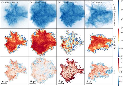
Top row: column density maps for simulations CG15-M4-G1, CG15-M5-G1, CG15-M5-G100, and GC16-Z1-G1. Middle row: the integrated intensity of the CO J = 2–1 transition for each simulation. Bottom row: the ratio, R21, of the integrated intensity of the CO J = 2–1 and J = 1–0 transitions for each simulation.
Comparing the first two columns of Fig. 1 reveals how changing the mass of the cloud alters their emission. By increasing the mass by a factor of 10, but maintaining the initial density, the size of the cloud is effectively doubled. Since the initial virial state of the simulations is the same, the initial velocity dispersion is roughly five times higher in CG15-M5-G1 than in CG15-M4-G1. As the sound speed of the gas is similar in the two simulations, the higher mass cloud has Mach number four to five times higher than the low-mass cloud. As a consequence, the higher mass cloud has a more intricate web-like structure with a larger number of turbulence-driven filaments. This is reflected in the synthetic images of the emission, since high-density regions correlate with high-intensity regions and vice versa, and as we shall see, this is an important factor in the distribution of R21.
The middle two columns compare the effect of varying the ISFR and the CRIR. In the high-ISRF/CRIR scenario, most of low-density, poorly shielded CO has been dissociated and the thin, low-density filaments have completely disappeared. More evident in the synthetic observations is how the apparent size of the cloud has been reduced by removing the low-intensity regions that were previously enveloping the entire cloud.
Finally, the bottom panels of Fig. 1 contain the R21 maps. As shown by Peñaloza et al. (2017), the area-weighted PDF of R21 has a bimodal distribution, with peaks centred at R21 ∼ 0.3 and R21 ∼ 0.7. In the first two columns, it is clear that the ratio map is mostly dominated by values of R21 ∼ 0.7; none the less, lower values of R21 are present in regions where W21 < few K km s−1. A very different picture is seen in the R21 map for CG15-M5-G100: towards the centre of the cloud R21 ∼ 0.5–0.7 but at the outskirts of the cloud R21 > 1. The high ISRF results in very high temperatures (T > 40 K) at the edge of very dense (n > 103 cm−3) regions of the cloud. In such circumstances, the τ = 1 surface for J = 1–0 can be deeper into the cloud than the τ = 1 surface for J = 2–1, which can result in R21 > 1. This effect was demonstrated in the 1D models of Sakamoto et al. (1994). It is worth noting that R21 can also be larger than 1 when the source of radiation is embedded within the cloud (see fig. 11 from Nishimura et al. 2015). Finally, when comparing R21 between CG15-M4-G1 and GC16-Z1-G1, it is clear that the morphology of the cloud (and thus the choice of turbulent velocity field) has an impact on the final value of R21.
Qualitatively, the ISRF and the CRIR have the biggest impact on R21's value and distribution. Their combined effects can hinder the accuracy of adopting a constant value of R21 ∼ 0.7 and therefore over- or underestimate the derived value for W10.
3.2 Systematic dependences of R21
The morphology of the cloud gives a qualitative picture of the impact that initial mass, turbulence, and the ISRF/CRIR have on the CO emission and the corresponding line ratios. In this section, we focus on the R21 line ratio. The different effects on the line ratio can be quantified by plotting the cumulative PDF of R21 weighted by integrated intensity (Fig. 2). The separation between the curves for each cloud shows how changes in environmental conditions impact the distribution and average value of R21. We reiterate here that low values of R21 (∼0.2–0.4) are associated with warm and diffuse gas, while high values of the R21 (∼0.6–0.8) are associated with cold and dense gas (Peñaloza et al. 2017).
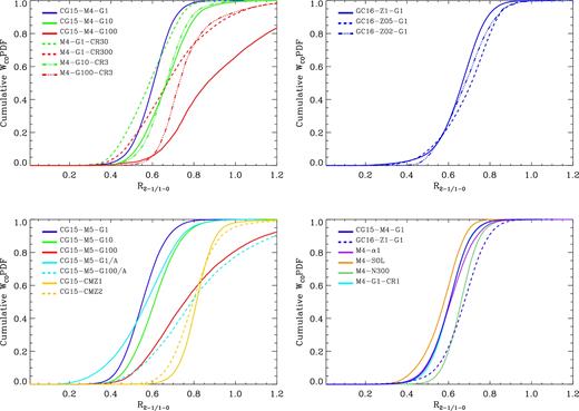
The cumulative PDF of R21 weighted by WCO for different sets of clouds grouped by variations in their physical parameters. Top-left panel: small clouds (104 M⊙), at solar metallicities and with varying ISRF, CRIR, or both. Top-right panel: small clouds (104 M⊙), with a solenoidal turbulent seed and varying metallicities. Bottom-left panel: large clouds (105 M⊙) with variations in both ISFR and CRIR. Cyan lines are clouds that start atomic and yellow lines clouds with initial n = 104 cm−3. Bottom-right panel: small clouds (104 M⊙) with changes to αvir, initial density, or the turbulent seed.
3.2.1 The ISFR and the CRIR
The top-left panel of Fig. 2 plots the cumulative PDF for a set of the low-mass clouds at solar metallicities. As the ISFR and the CRIR increase (solid lines), a larger fraction of the overall emission is associated with larger values of R21. In this case, almost half of the emission is associated with line ratio values of R21 > 1. As the ISRF increases, the unshielded molecular gas is fully dissociated, destroying most of the CO in the already diffuse gas and therefore resulting in no CO emission from these regions of the cloud. This is consistent with the fact that lower values of R21 (∼0.3) are associated with diffuse and warm areas of the cloud (Sakamoto et al. 1994; Peñaloza et al. 2017). Similar to CG15-M5-G100 (see the bottom-left panel in Fig. 2 and Fig. 1), values of R21 > 1 are correlated with CO emission originating from dense and hot gas at the edge of the cloud.
The dash–dotted lines represent the runs where only the ISRF field was increased while the CRIR was left unchanged. For these clouds, a large fraction of the emission is also associated with higher line ratios. However, a larger fraction (about 80 per cent) of the overall emission is associated with line ratios of R21 ∼ 0.6–0.8. A smaller CRIR means the dense gas within the shielded regions of the cloud is not being heated and therefore results in a more compact cloud. As such, most of the emission originates from dense and cold gas, which explains why a larger fraction of the emission is correlated with R21 ∼ 0.7.
On the other hand, the dashed lines represent the clouds where the ISRF was left constant while the CRIR was increased. In this case, about 50 per cent of the overall emission is correlated with lower line ratios (R21 ∼ 0.3–0.6). As shown by Glover & Clark (2016, see also Bisbas, Papadopoulos & Viti 2015; Bisbas et al. 2017), an increase in ζH can lead to a decrease in CO abundance. Even though the total abundance of CO has been reduced, it is still well shielded from the UV rays, resulting in emission originating from low-density gas and therefore associated with lower line ratio values. The effect of ζH on CO abundance will be more thoroughly discussed in Section 5. Additionally, the high CRIR will heat up dense regions of the cloud, thereby increasing the overall emission associated with higher line ratios (R21 > 0.9).
Finally, by comparing the bottom-left panel with the top-left panel, we can see that the compound effect of the ISRF and the CRIR does not depend on the cloud mass. Although the higher mass clouds tend to contain more filamentary structures (as discussed in the previous section), the combination of high ISRF and high CRIR results in heating which acts to smear out these high-density structures in both cases. As such, the variation in R21 as a function of ISRF + CRIR looks very similar in the high- and low-mass clouds.
3.2.2 Metallicity
The top-right panel of Fig. 2 plots the cumulative PDF of low-mass clouds (104 M⊙), with a solenoidal turbulent seed and varying metallicities. By reducing the metallicity, the conditions to form CO tend to only be achieved within dense cores (Glover & Clark 2016), which results in less CO emission from diffuse regions of the cloud. This can reduce the percentage of the low values of R21 that are associated with low-density gas, and indeed we see that in the case of Z = 0.2 Z⊙, there is almost no emission associated with R21 < 0.4.
We also see variations in the fractions of emission associated with the higher R21 values, although the overall effect is still quite small. These variations are likely due to the fact that as we decrease the metallicity, the abundances of both CO and H2 (the dominant collisional partner for CO) are both decreasing. As such, for a given total density of gas, the effective density of the species contributing to the emission is falling as we decrease the metallicity, which has the result of reducing R21. However, this is going to be partly offset by the fact that the gas is hotter at lower metallicities, which acts to raise R21, potentially explaining the overall small variation in the cumulative distribution of R21.
3.2.3 Mass and molecular fraction
The bottom-left panel of Fig. 2 contains all the clouds with total mass of 105 M⊙. The first point to notice is, by comparing the blue lines in the top- and bottom-left panels, that increasing the total mass of the cloud leaves the overall value and distribution of R21 relatively unchanged.
The effect of having an initially atomic cloud is on the fraction of the overall gas associated with lower line ratios, where about 40 per cent of the emission has values of R21 < 0.5 for clouds that start fully atomic. This tail at low values of R21 is correlated with a larger fraction of the emission coming from low-density/high-temperature regions. This is consistent with the idea that less molecular material at the beginning will delay the formation of CO (Glover & Clark 2012a), resulting in lower column densities of CO. Given that the impact of the ISRF and the CRIR is much stronger, as discussed above, the effect of initial f(H2) can be more easily observed at low ISRF, as the high-ISRF cases (solid red and dashed cyan) are relatively similar.
Finally, the two CMZ-like runs with an initial density of n = 104 cm−3 have a larger average value of R21, where most of the overall emission is associated with R21 ∼ 0.8. This is due to the fact that the initial density is well above the critical density of the first two rotational transition lines of CO (|$n_{\rm crit,1{\rm -}0} \approx 2000\ {\rm cm}^{-3}$|, |$n_{\rm crit,2{\rm -}1} \approx 10^4\,{\rm cm}^{-3}$|). As a result, the gas is well shielded from the ISRF and CO is easily excited. Since most of the emission is originating from high-density gas, this means that R21 will be centred near ∼0.7.
3.2.4 Turbulence, αvir, and initial density
As mentioned before, we have used clouds from Clark & Glover (2015) and Glover & Clark (2016); however, as can be seen in Table 1, these have slightly different initial conditions and environmental parameters. The bottom-right panel of Fig. 2 shows the clouds that explore variations in only these features. First, we must note that even though CG15-M4-G1 (blue solid line) and GC16-Z1-G1 (blue dashed line) have very similar initial conditions, the changes in turbulence, αvir, and initial density still noticeably change R21's distribution.
Glover & Clark (2016) adopted a solenoidal velocity field. Such a field has no compressive motions (|$\nabla \cdot {\boldsymbol u} = 0$|), resulting in more flocculent cloud (lower density) with a narrower PDF than is found for fields with similar Mach numbers and power spectra, but which contain compressive modes (Federrath et al. 2010). Consequently, a larger fraction of the emission originates from more diffuse gas, which is correlated with lower values of R21 in the clouds which adopt a solenoidal velocity field.
Increasing the value of αvir slightly increases the average value of R21. A larger kinetic energy results in higher Mach numbers, and thus more shock-compressed high-density regions. Although the higher αvir will also cause the clouds to expand, which would lower R21, there is not sufficient time for this to occur in our study; these clouds form stars more rapidly than the lower αvir clouds, which means we post-process them at an earlier time, before they have had the chance to expand. The net effect is that more gas is at high densities when we come to post-process, and thus a slightly larger fraction of the cloud will be associated with larger values of R21. Clearly, this effect will depend on time, which is beyond the scope of this study.
The green line shows, to a lesser extent, what was observed for CMZ-like clouds; increasing the initial density reduces the amount of diffuse gas and effectively increases the fraction of the gas associated with higher values of R21. The slightly different ζH between CG15-M4-G1 and GC16-Z1-G1 has very little effect; this can be seen by the cyan line where ζH = 1 × 10⁻¹⁷ s−1. Given that the variation in ζH is small, the change in R21 is not substantial. However, reducing the CRIR does slightly reduce the amount of emission associated with low line ratios. Finally, we note that the combined effect of turbulence, αvir, initial density, and slightly different ζH explains the different average value and distribution of R21 between CG15-M4-G1 and GC16-Z1-G1.
4 R21 FROM OBSERVATIONALLY UNRESOLVED CLOUDS
The previous section explained how variations in the initial conditions and in the surrounding environment affect both the mean value and distribution of R21. Moreover, effects on R21 can be associated with different regions of the cloud and are correlated with local physical properties of the gas. However, when comparing to observations in an extragalactic context, where R21 is used as a conversion factor, details about the varying value of R21 within molecular clouds are not known. In this context, one of our clouds will most likely be smaller than the observational beam size (cf. Schinnerer et al. 2013; Bigiel et al. 2016) and therefore the total intensity of one or more GMCs will be averaged within this beam. Therefore, to study R21 in the context of observationally unresolved clouds, we first take the area-weighted intensity average of each cloud for each rotational transition line and then take the ratio of the two averaged intensities. In this section, we focus on presenting the results from these area-averaged line ratios.
4.1 Averaged R21 for the whole cloud
In the previous section, it was suggested that varying the UV intensity has an impact on R21. We therefore plot the area-averaged value of R21 against the ISRF for all the clouds in Fig. 3.
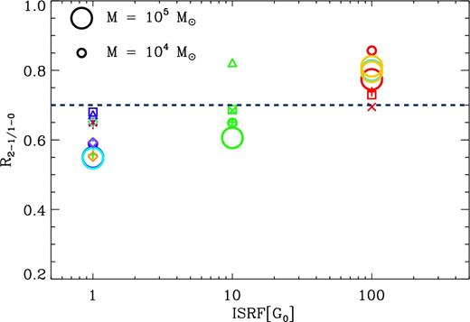
The averaged value of R21 for each cloud as a function of their respective ISRF (G0). Large circles represent clouds that have a mass of M = 105M⊙ and small shapes represent clouds with a mass of M = 104M⊙. Blue, green, and red shapes represent an increase of the ISRF and/or CRIR by 1, 10, or 100, respectively. Xs, squares, and triangles represent metallicities of Z⊙, 0.5 Z⊙, and 0.2 Z⊙, respectively. Large cyan circles denote an initial hydrogen fraction of f(H2) = 0. Yellow circles are the two runs with an initial number density of n = 104 cm−3. Plus signs are clouds where the ISRF and the CRIR have been varied independently. Diamonds are the additional runs plotted in the bottom-right panel of Fig. 2 and have the same colours. Finally, the dashed line represents the standard value used for converting W21 to W10. Note that we have not included GC16-Z02-G100 since the gas is not able to form enough molecular gas and therefore produces almost no CO emission.
First thing to note is that the averaged value of R21 covers a range of values between 0.5 and 0.9; this confirms that changes in the cloud's environmental conditions do influence the overall value of R21. An increasing ISRF is directly correlated with an increase in the average value of R21. Additionally, within each ISRF bin, there is appreciable scatter, which can be attributed to the different changes in environmental conditions discussed in the previous section. However, since the plot shows an averaged value for R21, the specific changes in the distribution of R21 are reduced making it harder to distinguish between different environmental effects.
Extragalactic observations often use R21 as a conversion factor rather than a diagnostic tool for GMC structure. In that context, the averaged dashed line in Fig. 3 represents the observationally derived and most commonly used value of R21 (Eckart et al. 1990; Casoli et al. 1991; Brand & Wouterloot 1995; Hasegawa 1997; Sakamoto et al. 1997; Sawada et al. 2001; Bigiel et al. 2008; Leroy et al. 2009; Barriault et al. 2011). This line lies in the middle of the scatter of R21 values of our clouds, suggesting that R21 ∼ 0.7 is a good first approximation for converting W21 into W10. None the less, it questions the reliability and robustness of the conversion factor, and suggests that adopting a fiducial value can lead to errors in derived quantities such as the total molecular gas. We discuss the consequences of such an approach, and possible solutions, in Section 5.
It is important to note that the agreement between our simulations and the accepted value of R21 improves when considering higher sensitivity cuts to our detection limits. Our synthetic observations have an already low emission cut of 0.01 K km s−1; when we impose a detection limit of 5 K km s−1 instead, the scatter is almost completely gone. Considering that the emission from diffuse gas associated with lower line ratios is always very faint, it follows that R21 ∼ 0.7 as sensitivity is reduced. This is a consequence of R21 being derived in a Galactic context where clouds are well resolved, and suggests that sensitivity plays an important role in how we have empirically derived the accepted value of R21.
4.2 CO emission as a probe of physical conditions
In Fig. 4, we plot |$\langle T_{\rm H_2}\rangle$| versus 〈TCO〉 where every point represents a cloud, and the points have the same shape and colour as in Fig. 3. First thing to note is that the temperature of the molecular cloud – as defined by the H2 – increases as we increase the ISRF and/or CRIR, which is to be expected. However, this increase in temperature is only reflected in |$\langle T_{\rm H_2}\rangle$|, while CO-rich gas never reaches temperatures above T ∼ 40 K. As such, the CO emission from the cloud is only tracing the temperature variations in a sub-set of the full H2 molecular gas. This is easily understood since the bulk of the CO gas is within well-shielded regions where temperature of the gas is low and the densities are above ncrit. This is not the case for H2, which is present in more diffuse regions where the temperature range can be higher (see also Walch et al. 2015 and Glover & Smith 2016, who find similar results in larger scale simulations of the ISM).

One notable exception is when considering the two CMZ clouds (yellow circles); in this case, TCO and |$T_{\rm H_2}$| are very similar. Since the initial density of these clouds is much higher, this results in most of the gas being well shielded and therefore at similar temperatures. Since the densities are high enough to excite CO, the CO emission is well correlated with the overall temperature of the gas. As was mentioned in the previous section, this is also reflected in the small variations of R21.
4.3 Alternative line ratios
Having created synthetic observations for the lowest three emission lines of CO's rotational ladder, it is a simple task to consider other ratios between these lines as possible conversion factors. In this section, we explore the ratios R32 and R31, which have both been employed as conversion factors in extragalactic studies.
4.3.1 R32
We first consider R32, that is the ratio between the third (J = 3–2) and second (J = 2–1) rotational levels of CO. In order to judge how R32 varies, we plot a similar figure to Fig. 3, where we take the average intensities of each line for each cloud and then calculate the line ratio. This is shown in Fig. 5.

In this case, the overall scatter is considerably larger than it was for R21, and our results are all above the standard value of R32 = 0.5 (Vlahakis et al. 2013). At the same time, R32 is also highly dependent on the changes in the ISRF as demonstrated by the increase in the averaged value of R32 with increasing ISRF. When we examine the properties of the individual clouds within each ISRF bin, the spread seems to be correlated with the initial density of the simulations. Considering that the critical densities of J = 2–1 and J = 3–2 are of the same order of magnitude (ncrit ∼ 104 cm−3), then a larger fraction of R32's distribution originates from regions that are sub-critically excited, i.e. n < 104 cm−3 with lower initial densities. This explains why the value of R32 is larger for most of the GC16 clouds that have a slightly larger initial density.
Finally, the CMZ-like clouds have a larger value of R32 ∼ 0.9. Since the cloud starts with an initial density of n = 104 cm−3, which is close to the critical densities for both transitions, this results in comparable emission rates from both lines and therefore a ratio closer to unity.
4.3.2 R31
In Fig. 6, we look at the variations of R31, that is the ratio between CO's third (J = 3–2) and first (J = 1–0) rotational emission lines. The scatter for R31 is similar to R32, and we also see an increase in the average value with increasing ISRF. However, the value of R31 is more evenly spread in each ISRF bin, suggesting that R31 is slightly more susceptible to changes of environment and initial conditions of GMCs.

R31 has a higher variability due to the larger difference in excitation conditions for both lines. The critical density of the J = 3–2 emission line is ncrit = 3.6 × 104 cm−3, which is over an order of magnitude higher than the J = 1–0 line. Furthermore, the difference in energy required to excite both lines is ∼27.7 K, which is quite significant when considering the low-temperature environments of dense regions within GMCs. This explains why at lower ISRF R31 is small, since a significant amount of emission is arising from diffuse regions where the J = 1–0 line is easily excited but J = 3–2 is not. On the other hand, at high ISRF both lines will be excited in dense regions, since the clouds are warmer, and in addition, the dissociation of the CO in the diffuse gas will lower the contribution to the emission from J = 1–0. Overall, the net effect is to increase the value of R31.
R31 is usually taken to be R31 = 0.5 ± 0.2. Our results show that the scatter of the average value for different clouds is just over the expected error for R31. However, the results in Fig. 6 also suggest that using R31 = 0.5 can considerably underestimate or overestimate the amount of emission associated with W10, and in turn, any derived properties of the source. At the same time, this suggests that if the value of the ISRF is known, a better constrained conversion factor with a smaller error can be used. We shall explore this in the following section.
5 DISCUSSION
5.1 XCO in unresolved clouds
The results presented in Section 4 show the dependence of the line ratios on the properties of the gas in the clouds, and the environmental conditions to which the clouds are exposed. In the Milky Way, where it is possible to resolve clouds, the line ratios can serve as a probe of the physical conditions in the cloud. We have also shown that the area-averaged line ratios arising from unresolved clouds also show significant variation. This can have implications for how they are used as conversion factors from the J = 2–1 and J = 3–2 lines to the more commonly used J = 1–0 transition that is used in the X-factor. In this section, we explore how these variations in R21 and R31 affect our derivations of physical cloud properties.
Before doing so, we reproduce fig. 4 from Clark & Glover (2015) where they plotted the value of XCO for each cloud against the ‘star formation rate’, which is a proxy for changes in the ISRF and CRIR. In this case, we plot against the ISRF as well as include additional clouds that were not studied in Clark & Glover (2015, see Fig. 7). Additionally, we have only included clouds with Z = Z⊙, since XCO is empirically derived from observations within the Milky Way and therefore intrinsically assumes a solar-like metallicity. It is important to note that this plot may look slightly different from fig. 4 of Clark & Glover (2015). This is because our radiative transfer approach here includes the refinement routine described in Peñaloza et al. (2017) and the Sobolev–Gnedin approximation described in Appendix A. When compared, the results presented here systematically lower the value of XCO, making these results closer to the typically used value.

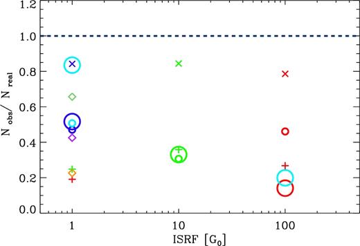
In Fig. 8, the Nobs/Nreal ratio against the ISRF is plotted. When calculating Nobs, we have used the XCO = 2 × 1020 cm−2 K km s−1 as given by Bolatto et al. (2013) and R21 = 0.7. From this figure, it becomes evident that the amount of molecular gas derived from W21 can easily be underestimated. This can be understood when comparing with Fig. 7 where at high ISRF the standard value of XCO will underestimate the total column of H2. On the other hand, Fig. 3 shows that using an average value of R21 = 0.7 will overestimate the amount of W10 at high ISRF. Effectively, this compensates the existing biases of both conversion factors to some extent; however, this is not enough to avoid underestimating the amount of H2 due to the high errors in XCO. This is also the case for the green and red plus signs at ISRF = 1; they correspond to the high-CRIR runs, where XCO is also underestimated.
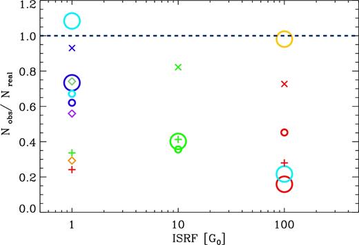
The Nobs/Nreal ratio against ISRF for all the clouds using the same labels as in Fig. 3, where Nobs is calculated using R21. Note that clouds with metallicities of Z ≠ Z⊙ are not included.
At lower ISRF, the discrepancies between Nobs and Nreal arise from R21, since at lower ISRF XCO is well within the accepted value. From Fig. 3, we can see that using R21 = 0.7 effectively underestimates the amount of W10 and therefore the total column density of H2. This effect is even stronger when using R31 instead of R21, which is seen in Fig. 9 where we use R31 = 0.5 to calculate Nobs.
Similar to Fig. 8 but using R31 instead of R21.
Finally, even though our results suggest that R21 = 0.7 is a good first approximation for a conversion factor between W21 and W10, the uncertainties and degeneracies surrounding R21 still have a significant effect on Nobs. This is also true for R31, where the effect on Nobs is even larger given that the accepted value for R31 is a lower limit according to our results. Alternatively, if the surrounding ISRF could be constrained – for example, by looking at dust SEDs – then the average values in Fig. 3 (and Fig. 6 for R31) for each ISRF bin could be used to improve the estimate in the value of R21 and R31. In principle, this can lead to better true column density of molecular material. Whether this would yield a more accurate value of Nobs would depend on the uncertainties on the method used to obtain the ISRF and is beyond the scope of this paper.
5.2 R21 as a probe of CO abundance
As discussed in Section 3, variations in the strength of the ISRF and the CRIR affect R21 in different ways. Since we are interested in quantifying the effect of the ISRF and the CRIR on the state and abundance of molecular gas, we will focus on the following four clouds CG15-M4-G1, M4-G1-CR100, M4-G100-CR1, and CG15-M4-G100. We then plot the fractional abundance of CO and H2 as a function of the average number density of the gas for each cloud. This is shown in Fig. 10 , where the solid lines represent the H2 abundance fraction and the dashed lines CO abundance fraction.
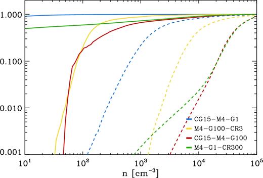
Each coloured line represents a different simulation. Solid lines track, as a function of number density, the fraction of the mass of H in the form of H2 while dashed lines track the fraction of the mass of C in the form of CO.
When looking at the cloud with high ISRF, the fraction of CO abundance (dashed yellow line) increases quickly; this is because once the CO is well shielded, the production of CO is efficient. As a result, the emission coming from these high-density regions will be bright and well correlated with high values of R21. On the other hand, when looking at the high-CRIR cloud, the fraction of CO abundance (dashed green line) starts increasing at similar number densities (∼103 cm−3), however, at a much slower rate. This is because the CO production is being constantly hampered by the cosmic rays which are not attenuated. As such, the emission from these regions will be faint due to the low abundance of CO; more importantly R21 will have values around ∼0.3. In addition, the increase in the CRIR will heat up the gas and therefore slightly increase the average value of R21 (see Fig. 3).
A recent paper by Bisbas et al. (2017) studied how increasing the CRIR can be important in destroying CO. In fig. 11 of this paper, they compare the CO/H2 fraction as a function of number density, for varying CRIR. We reproduce this figure with our own set of simulations for which the CRIR is increased in the same way. (Note that to better compare to their results, we ran an additional simulation with ζH = 3 × 10⁻¹⁴ s−1 that was not included in our initial setup.) Our results show a similar trend where the CO/H2 abundance ratio decreases with increasing CRIR (see Fig. 11).
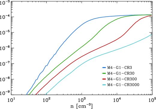
Illustration of how CO/H2 abundance ratio changes with average number density.
The effect of CRIR on the abundance of CO will have a direct impact on the CO emission and therefore how much molecular gas can be traced within GMCs. Even though the total CO emission is reduced, our synthetic observations show that the changes in abundances seen above can be traced to some extent when looking at the resolved integrated intensities and R21 of these clouds (see Fig. 2). One caveat to keep in mind when considering these results is that our models have a constant CRIR throughout the whole cloud – cosmic rays are not attenuated and therefore able to reach the densest regions of the cloud. Whether this is an accurate approximation is beyond the scope of this study, and therefore the reader should keep this in mind when interpreting these results.
6 CONCLUSIONS
We have studied a range of numerical models of molecular clouds, in which the initial cloud parameters, and properties of the ISM, were systematically varied. We performed radiative transfer calculations on the simulations just before the onset of star formation in each case, to create synthetic CO line emission cubes for all clouds. We used these synthetic observations to study the impact of environment on CO line emission and CO line ratios. Our main findings can be summarized as follows.
The value of R21 and its correlation with dense/cold and warm/diffuse gas allow it to act as a probe of the conditions of the gas within GMCs. From all the environmental changes studied, variations in the ISRF and the CRIR have the largest impact on the average value and the cumulative PDF of R21.
The dependence of different line ratios (R21, R32, and R31) on environment can also be observed when looking at unresolved clouds where the total emission is averaged. Our results suggest that the accepted values for R21 and R31 are a good first approximation. At the same time, the scatter around the accepted value (∼±0.2) suggests that careful consideration should be had when using them as conversion factors, especially given the high dependence on the ISRF.
When calculating the column density of H2 molecular gas of GMCs, it is important to consider the biases of XCO and line ratios R21 and R31. At a high ISRF (G0 = 100), XCO will underestimate |$N_{\rm H_2}$|. This is only slightly compensated by the bias line ratios have at high ISRF. On the other hand, since at low ISRF (G0 = 1) XCO is well constrained, the errors in |$N_{\rm H_2}$| come from line ratios underestimating the total amount of emission from the J = 1–0 transition line.
Cosmic rays can help regulate the total CO abundance within GMCs. When ζH = 3 × 10⁻¹⁷ s−1, the CO-to-H2 abundance ratio is ∼10−4 at densities of ∼103 cm−3. As ζH is increased, the CO-to-H2 fraction is considerably reduced reaching values of only ∼10−5 at densities of ∼105 cm−3 for rates of ζH = 3 × 10⁻¹⁴ s−1. This has a direct impact on the CO emission and on the average value and distribution of R21.
Acknowledgements
PCC acknowledges support from the Science and Technology Facilities Council (under grant ST/N00706/1) and the European Community's Horizon 2020 Programme H2020-COMPET-2015, through the StarFormMapper project (number 687528). SCOG and RSK acknowledge financial support from the Deutsche Forschungsgemeinschaft via SFB 881, ‘The Milky Way System’ (sub-projects B1, B2, and B8) and SPP 1573, ‘Physics of the Interstellar Medium’. They also acknowledge support from the European Research Council under the European Community's Seventh Framework Programme (FP7/2007-2013) via the ERC Advanced Grant STARLIGHT (project number 339177).
REFERENCES
APPENDIX A: SOBOLEV–GNEDIN APPROXIMATION
The Sobolev approximation, most commonly known as the large velocity gradient (LVG) approximation, is widely used when calculating the level populations of a gas within GMCs. In the original paper, Sobolev (1957) studied the idea that emission coming from gas within a moving medium will be Doppler-shifted before it can be reabsorbed and therefore escapes. Whether a photon escapes or not is determined by the velocity gradient (|$|\nabla \boldsymbol {v}|$|), i.e. the larger the |$|\nabla \boldsymbol {v}|$| is, the smaller is the volume where the photon can be reabsorbed. radmc-3d already makes use of the Sobolev approximation when calculating level populations; the detailed implementation can be found in Shetty et al. (2011).
Now consider a scenario in which |$|\nabla \boldsymbol {v}|$| is small but the change in density, i.e. the density gradient (|∇ρ|), is high. According to equation (A2), τ would be high and therefore the probability of a photon escaping would be low. However, given that |∇ρ| is higher, the escape probability of the photon should be higher, yet equation (A2) does not consider |∇ρ| and therefore the escape probability is unchanged. For the GMCs considered in this study, we can foresee different cloud regions where this scenario is likely: dense cores can have low velocity dispersions, yet can have very steep density gradients. In effect, the LVG is a local approximation, in that it constructs a length-scale based on local properties. These local properties, such as density, temperature, etc., are then assumed to be held constant over this length-scale, allowing us to derive an optical depth. If, however, the density varies rapidly, then the LVG approximation makes an error. Thankfully, it is relatively simple to improve this approximation.
A1 Gnedin length approximation
The resulting optical depth will then be used in equation (A1) to calculate the escape probability.
A2 Implementation and testing
We have used the underlying framework of radmc-3d and implemented the Gnedin approximation, as described above, as an improvement to the already-present Sobolev approximation. In order to test this method, we set up a test scenario that highlights the difference between LTE (local thermodynamic equilibrium), LVG, and LVG+ (Sobolev–Gnedin approximation).
We set up an input grid of 10 by 10 by 2; Fig. A1 shows the position–position–position cube that was used as an input into radmc-3d. All the cells in the front slice have the same physical properties and will therefore have the same intrinsic emission in a scenario where |$|\nabla \boldsymbol {v}|$| or |$|\nabla \boldsymbol {\rho }|$| are not considered. The back slice serves to calculate the velocity and density gradients used to obtain the optical depth of each cell in the front slice. To keep the setup simple, we increase |$|\nabla \boldsymbol {v}|$| only on the x-axis while keeping |$|\nabla \boldsymbol {\rho }|$| constant. Conversely, we increase |$|\nabla \boldsymbol {\rho }|$| while keeping |$|\nabla \boldsymbol {v}|$| constant on the y-axis. The increase in the gradient is taken with respect to the values of density and velocity in the front slice. These are such that dv = dρ will be the same whenever x = y. Additionally, to avoid confusion, we set the temperature of each cell in the back slice to be T = 0 K so that these cells have no emission.
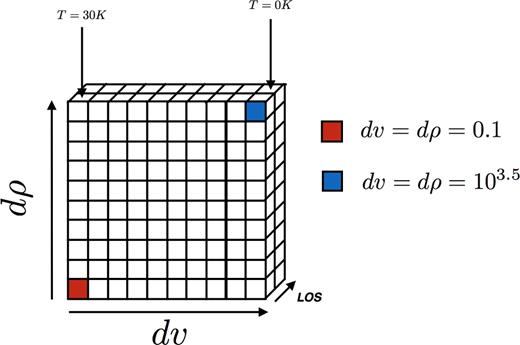
The setup of the grid used as an input for the radiative transfer. All the cells in the front slice have the same density, temperature, and velocity. The back slice has a temperature of 0 K. Densities and velocities take a value according to dv or dρ, which are increased such that dv = dρ over the diagonal. dv is increased accordingly over the x-axis and dρ over the y-axis.
Given the purpose of this paper, we perform the radiative transfer for CO J = 1–0 but in principle the method works for any other molecule or line. Additionally, we create three different cubes for three different densities of the front slice (n = 50, 100, and 500 cm−3). We run three radiative transfer simulations for each cube; each of these uses either LTE, LVG, or LVG+. The resulting integrated intensities for each run for each cube are shown in Fig. A2.
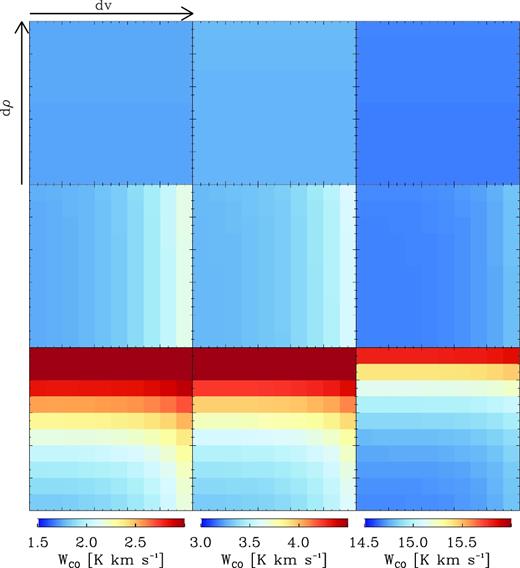
The integrated intensities of CO J = 1–0 for each run on each cube. Each row has a different method for calculating level populations: top = LTE, middle = LVG, bottom = LVG+. Similarly, each column has a different number density for the front slice, left: n = 50 cm−3, middle: n = 100 cm−3, right: n = 500 cm−3. Note that even though the colours are similar, the colour bar for each column is different.
As expected, changing the method for calculating the population levels makes a big difference in the final image. Since the density and temperature of each cell are exactly the same, assuming LTE results in the integrated intensity for each cell also being the same. This is because LTE uses no information of the gradient surrounding the cell to calculate the level populations. For the LVG scenario, we can definitely see a change in intensity over the x-axis, which corresponds to an increase in |$|\nabla \boldsymbol {v}|$|. However, not taking |∇ρ| into account results in the intensity being exactly the same on the y-axis. Finally, when using the LVG+ method, both changes on |$|\nabla \boldsymbol {v}|$| and |∇ρ| are reflected in the final intensity of each cell.
One important thing to keep in mind when looking at these results is why increasing the gradient results in an increase in intensity rather than a decrease. The reason is that the background radiation and the high temperature of the cell cause higher levels to be radiatively pumped. These will then quickly cascade down to the ground state, i.e. J = 1–0, causing it to be much brighter. The reason behind this is that for lower temperatures, the difference between cells is very small and hard to see. This should not be a problem since our interest is to test that the method works. In the next section, we will show how using LVG+ changes the integrated intensities of one of our clouds.
A3 Result comparison
Even though we tested that LVG+ works, it is important to check whether this new method has any significant effect on a more realistic system such as our numerically simulated clouds. To check this, we performed two radiative transfer simulations on CG15-M4-G1, one using LVG and another using LVG+. The integrated intensities of these two runs are shown in Fig. A3.
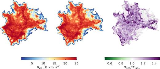
The image on the left shows the integrated intensity for CG15-M4-G1 with an LVG treatment while the middle image does so for LVG+. The image on the right is the ratio of LVG/LVG+ integrated intensities.
At first glance, it seems that the difference between LVG and LVG+ is negligible. However, when taking the ratio between the both, we can see that the brightness of the cloud definitely changes when using LVG+. For most regions of the cloud, the brightness is reduced; none the less, there are still regions that can either become brighter or remain the same. It then follows that considering changes in the local density does play an important role when calculating the level populations and total emission of a system. This illustrates how small changes in the physical conditions of the gas and the interplay with the surrounding environment can lead to changes in the total emission.
