


Abstract
Optical spectra of the 2006 outburst of RS Ophiuchi beginning one day after discovery to over a year after the outburst are presented here. The spectral evolution is found to be similar to that in previous outbursts. The early-phase spectra are dominated by hydrogen and helium (i and ii) lines. Coronal and nebular lines appear in the later phases. Emission line widths are found to narrow with time, which is interpreted as a shock expanding into the red giant wind. Using the photoionization code cloudy, spectra at nine epochs spanning 14 months after the outburst peak, thus covering a broad range of ionization and excitation levels in the ejecta, are modelled. The best-fitting model parameters indicate the presence of a hot white dwarf source with a roughly constant luminosity of 1.26 × 1037 erg s−1. During the first three months, the abundances (by number) of He, N, O, Ne, Ar, Fe, Ca, S and Ni are found to be above solar abundances; the abundances of these elements decreased in the later phase. Also presented are spectra obtained during quiescence. A photoionization model of the quiescent spectrum indicates the presence of a low-luminosity accretion disc. The helium abundance is found to be subsolar at quiescence.
1 INTRODUCTION
RS Ophiuchi (RS Oph) is a recurrent nova that has had nova outbursts in 1898, 1933, 1958, 1967 and 1985 (Rosino 1987), with possible outbursts in 1907 (Schaeffer 2004) and 1945 (Oppenheimer & Mattei 1993). It is a fast nova with t3 = 8–10 d, and the optical spectrum is characterized by strong coronal and other high-excitation lines that reach a peak around 60 d after maximum (e.g. Rosino 1987; Anupama & Prabhu 1989). The outbursts occur due to thermonuclear runaway (TNR) on a massive white dwarf (WD) surface that has accreted matter from its red giant companion star (Starrfield, Sparks & Truran 1985; Yaron et al. 2005). The fast-moving nova ejecta interact with the slow-moving red giant wind, leading to the formation of shocks (Bode & Kahn 1985, O'Brien & Kahn 1987). This leads to the formation of coronal lines, and also the narrowing of the emission lines (e.g. Gorbatskii 1972, 1973; Snijders 1987; Anupama & Prabhu 1989; Shore et al. 1996). There is a remarkable similarity between the optical light curves and spectra from different outbursts (Rosino 1987). So far, the 1985 outburst has been one of the best studied events, being recorded from X-rays to radio wavelengths (Bode 1987 and references therein).
The sixth recorded outburst of the recurrent nova RS Oph was discovered on 2006 February 12.83 (Narumi et al. 2006). It offered another chance for multiwavelength observations, and has been studied in detail in several wavelength regimes; e.g. in X-rays (e.g. Bode et al. 2006; Sokoloski et al. 2006), in the optical (Buil 2006; Fujii 2006; Iijima 2006; Skopal et al. 2008), in the infrared (IR) (e.g. Das, Banerjee & Ashok 2006; Monnier et al. 2006; Evans et al. 2007; Banerjee, Das & Ashok 2009) and in the radio (e.g. O'Brien et al. 2006; Kantharia et al. 2007; Rupen, Mioduszewski & Sokolowski 2008). The X-ray results clearly detect an X-ray blast wave that expands into the red giant wind. The temporal evolution of the shock wave was traced from XRT observations from the Swift satellite (Bode et al. 2006) and the Rossi X-ray Timing Explorer (RXTE) observations (Sokoloski et al. 2006). A similar shock has been detected from the evolution of the line widths in the near-IR spectra of the 2006 outburst (Das et al. 2006). The 2006 outburst also showed a similarity to the previous outburst, with some differences, especially in the X-rays and radio.
In this paper, we present the evolution of the optical spectrum of RS Oph over 14 months following the 2006 outburst based on spectra obtained using the 2 m Himalayan Chandra Telescope (HCT), Hanle, India and the 2.3 m Vainu Bappu Telescope (VBT), Kavalur, India. We have also modelled the observed spectra with the photoionization code cloudy. From the best-fitting spectra, we have estimated physical parameters such as luminosity, temperature, elemental abundances etc. associated with the RS Oph system.
2 OBSERVATIONS AND DATA REDUCTION
The observations of RS Oph began on 2006 February 13, one day after the outburst discovery, and continued well after the nova had reached quiescence. Low-resolution spectra were obtained using the HCT and occasionally with the VBT, while high-resolution (R ∼ 30 000) spectra were obtained with the VBT in the immediate post-maximum phase (2006 February 14 and 19). The HCT spectra were obtained using the Himalaya Faint Object Spectrograph Camera (HFOSC) through grism #7 (R ∼ 1500) and grism #8 (R ∼ 2200), covering the wavelength ranges of 3400–8000 Å and 5200–9200 Å respectively. The high-resolution VBT spectra were obtained covering the wavelength ranges of 4000–8000 Å using the fibre-fed Echelle spectrograph. Table 1 gives the dates of observations. We adopt the date of the maximum as 2006 February 12.83 (JD 245 3779.330).
Journal of observations of RS Oph during 2006.
| Date | Telescope | Instrument |
|---|---|---|
| Feb 13 | HCT | HFOSC |
| Feb 14 | VBT | Echelle |
| Feb 15 | HCT | HFOSC |
| Feb 16 | HCT | HFOSC |
| Feb 17 | HCT | HFOSC |
| Feb 18 | HCT | HFOSC |
| Feb 19 | VBT | Echelle |
| Feb 20 | HCT | HFOSC |
| Feb 21 | HCT | HFOSC |
| Feb 24 | HCT | HFOSC |
| Feb 26 | HCT | HFOSC |
| Feb 27 | HCT | HFOSC |
| Feb 28 | HCT | HFOSC |
| Mar 2 | HCT | HFOSC |
| Mar 10 | HCT | HFOSC |
| Mar 12 | HCT | HFOSC |
| Mar 14 | HCT | HFOSC |
| Mar 16 | HCT | HFOSC |
| Mar 21 | HCT | HFOSC |
| Mar 24 | HCT | HFOSC |
| Apr 1 | HCT | HFOSC |
| Apr 3 | HCT | HFOSC |
| Apr 24 | HCT | HFOSC |
| Apr 26 | HCT | HFOSC |
| May 3 | HCT | HFOSC |
| May 26 | HCT | HFOSC |
| Jun 1 | HCT | HFOSC |
| Jul 1 | HCT | HFOSC |
| Jul 4 | HCT | HFOSC |
| Jul 19 | HCT | HFOSC |
| Aug 18 | HCT | HFOSC |
| Oct 17 | HCT | HFOSC |
All spectra were reduced in the standard manner using the various tasks under the iraf package. The spectra were bias subtracted, flat-field corrected and the spectrum extracted using the optimal extraction method. The HFOSC spectra were calibrated using the FeAr calibration source for the blue region, and the FeNe calibration source for the red region. Spectroscopic standards obtained during the same night were used for instrumental response correction. The blue and red spectra of the same night were combined and spectra obtained on a relative flux scale, which were then flux calibrated using the photometric magnitudes published in the literature. All spectra were then de-reddened using E(B − V) = 0.71. The VBT Echelle spectra were wavelength calibrated using the ThAr source. These spectra are not flux calibrated.
3 EVOLUTION OF THE OPTICAL SPECTRUM
3.1 The early phase: days 1 to 15
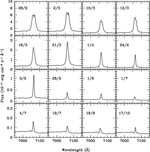
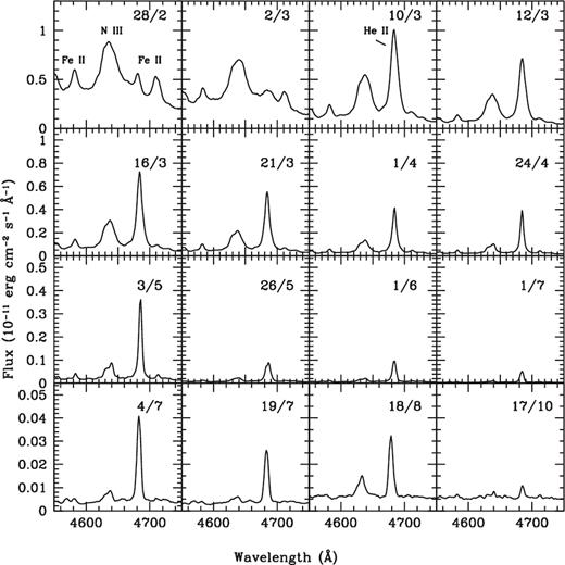
One day after the maximum, the spectrum is dominated by broad emission lines due to H, N, Ca ii (IR), Na i and O i. Weak P Cygni absorption features are seen associated with the emission lines. The nova appears to be in the ‘fireball expansion’ phase. About 5 d after maximum, P Cyg absorption features associated with the broad emission are absent and the emission line widths are narrower. The continuum appears bluer. The prominent lines are due to H and Fe ii. An [Ar x] 5535 line could be weakly present. The strength of the O i 8446 line has increased while the strength of the Ca ii IR lines has decreased. [Fe x] 6374 begins to appear around day 8. Sharp [O iii] 4959, 5007, [N ii] 5755 appear around day 15. [Fe xi] is probably present on day 15. These lines most probably arise from the ionized red giant wind. In the spectra of days 14–16, the He i lines show a double peaked profile. The spectra are shown in Figs 1 and 2.
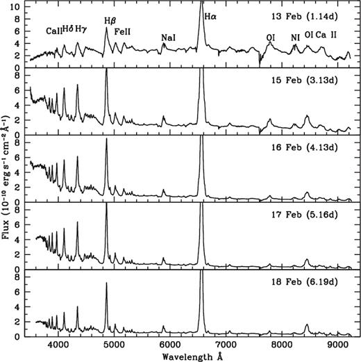
Spectra of RS Oph during 2006 February. The most prominent features are those due to H, Fe ii and Ca ii. The H α line has been truncated so that the weaker lines are seen properly.
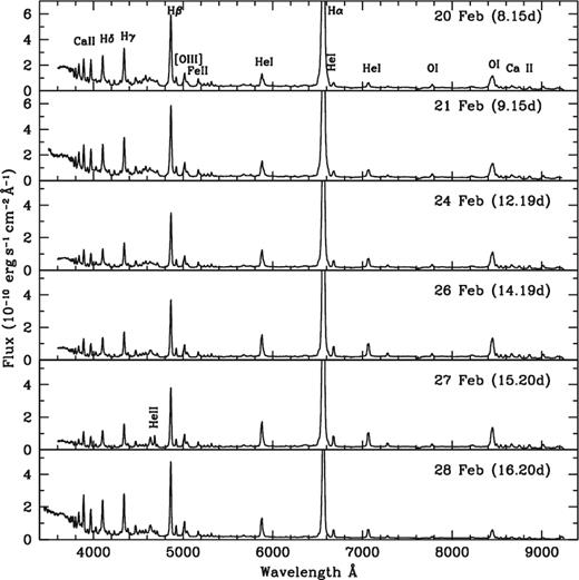
Spectra of RS Oph during 2006 February (continued). Note the emergence and strengthening of the He ii 4684 Å line during days 8–15, and the sudden decline on day 16.
RS Oph was detected in the 14–25 keV band of the Swift XRT and in the 3–5 keV and 5–12 keV bands of the RXTE all-sky monitor over ∼0–5 d, with an increasing flux (Bode et al. 2006; Sokoloski et al. 2006). The presence of the coronal lines in the optical spectrum during the very early phase appears to be consistent with the hard X-ray detection. The increase in the blue continuum is also consistent with the increase in the X-ray flux.
The high-resolution spectra of day 1 show sharp, narrow P Cygni emission features superimposed over the broad emission features (see Fig. 3). The P Cyg absorption, which originates in the circumstellar red giant wind, indicates a velocity of ∼20 km s−1. The absorption decreased in strength around day 7, similar to the broad absorption component. The wind emission is dominated by Fe ii emission lines. The spectra clearly show the Na ID interstellar absorption components as well as several diffuse interstellar bands between 5690 Å and 5870 Å at 5705, 5778, 5780, 5797, 5844 and 5849 Å (Josafatson & Snow 1987). Of these, the narrow bands at 5780, 5797 and 5849 Å are correlated with interstellar reddening. Using the average of the 5797 Å narrow band equivalent width of 0.109 ± 0.01 Å, E(B − V) = 0.75 ± 0.05 is estimated.
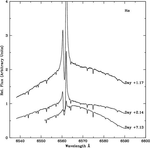
The H α line in the high-resolution spectra during days 1–7. The emission from the nova ejecta is broader than the wavelength covered by the order. The plot shows the narrow P Cygni component from the circumstellar material. Note the decrease in the strength of this component by day 7.
3.2 The high-excitation phase: days 16 to 80
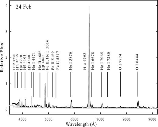
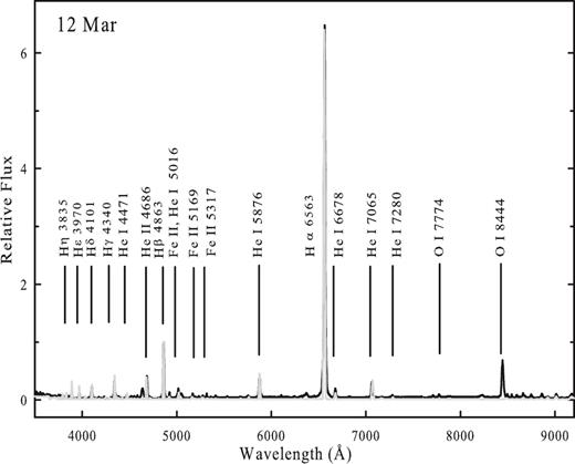
This phase is marked by a decrease in the strength of the permitted lines, and the strengthening of high-excitation lines. The Fe ii lines fade, while the He i lines develop and strengthen with time, and by ∼ day 25, the spectrum is dominated by H and He (i and ii) lines (Fig. 4). Also, O i 8446 becomes stronger than O i 7774. The emergence of the He ii lines is consistent with the onset of the supersoft X-ray phase (SSS phase) that commenced about 30 d after outburst (Osborne et al. 2011). Although a few coronal lines began developing as early as day 8, the onset of the coronal phase appears to be around day 25, with all the coronal lines, due to [Fe x], [Fe xi] and [Fe xiv] being strongly present, and strengthening with time. The coronal phase peaks around 60–70 d after maximum, similar to the previous outbursts (Anupama & Prabhu 1989).
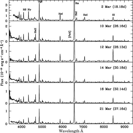
Spectra of RS Oph during 2006 March. The Fe ii lines have weakened, and the lines due to He have strengthened. Also note the strengthening of the coronal lines and O i 8446 Å.
The line profiles show multiple components. The widths of the emission lines continue to decrease with time. After around 70 d, the [O iii] line width becomes similar to those of other lines, and the spectrum is dominated by Balmer, He ii, coronal and other high-excitation lines. O i 8446 shows a two-component – a broad and a narrow component – structure. By day 80, the [O iii] lines are strengthening, and the O i 8446 Å two-component structure continues. The spectra are shown in Fig. 5.

Spectra of RS Oph during 2006 April–June. The coronal and other high-excitation lines are strong during this period.
3.3 The nebular phase: beyond day 100
The nebular phase began by day 100, and the nova is well into the nebular phase by ∼135 d. The nebular lines are broader compared to the recombination lines. The coronal lines have weakened in strength. Other nebular lines such as [Ca ii] 7323 begin to appear. Fe ii and N i lines are absent or very weak. The nebular lines get stronger between days 140–160 and are broader than other lines. H α shows asymmetric broad wings, with a velocity similar to those of the nebular lines. A contribution from the giant secondary is seen by day 140, as indicated by the presence of TiO absorption bands. These spectra can be seen in Fig. 6.
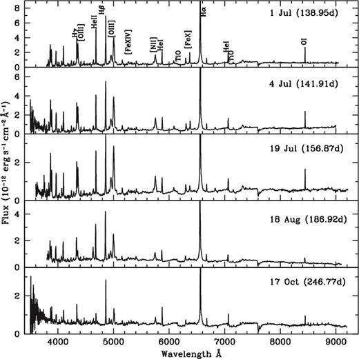
Spectra of RS Oph during 2006 July–October. The nova has reached the nebular phase during this period. TiO absorption features are present.
4 DESCRIPTION OF SOME EMISSION LINES
4.1 Emission line velocities
The emission line widths are found to narrow with time. The hydrogen Balmer lines indicate the following velocities: 4200 km s−1 (+1 d); 3800 km s−1 (+3 d); 2000 km s−1 (+5 d); 1060 km s−1 (+18 d); 740 km s−1 (+31 d); 332 km s−1 (+70 d). Fig. 7 shows the evolution of the emission line velocity. The velocities vary as t−0.4 for t < 5 d and t−0.66 during t = 5–70 d. This phenomenon is seen in the near-infrared lines as well and has been generally interpreted as free expansion of the shock front during the first four days and a deceleration phase thereafter (Das et al. 2006; Banerjee et al. 2009). These findings are also consistent with the X-ray observations (Bode et al. 2006; Sokoloski et al. 2006).
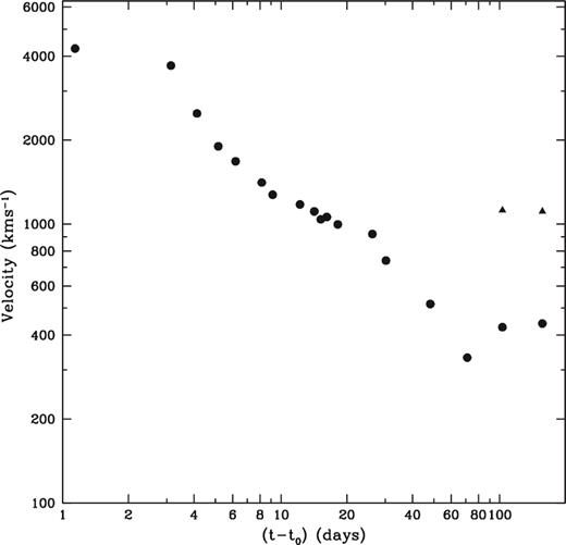
Velocities in the RS Oph spectra. It can be seen that the free expansion phase lasted only 4 d. The sharp fall in velocity after that is due to the shock wave generated when the high-velocity nova ejecta interact with the slow-moving red giant wind. Note the increase in the velocity after day 80.
A slight increase in the emission line width of the recombination lines is seen after day 80. The nebular lines are broader than the recombination lines, with a velocity v ∼ 1500 km s−1 compared to v ∼ 400 km s−1 for the recombination lines.
4.2 Oxygen lines
The O i 8446 Å line is stronger than the 7774 Å line on all days, implying that Ly β fluorescence is the dominant excitation mechanism. The evolution of these two lines can be seen in Figs 8 and 9. The [O i] 6300 and 6364 lines are best seen in spectra starting in 2006 May. The O iv 6106 and 6182 lines are seen from 2006 March 10 onwards and are clearly identifiable till 2006 July. There is a hint of the [O iii] 4363 line in the spectra obtained from 2006 February 21 onwards. It is clearly seen on 2006 April 1. On 2006 May 26 it is seen to be as strong as H γ. It fades thereafter, but is seen till 2006 August 18. There is no sign of this line in the 2006 October 17 spectrum. The evolution of this line can be seen in Fig. 10. Similarly, there are indications of the [O iii] 4959 and 5007 lines from 2006 February 20 onwards. They are clearly seen on 2006 April 1, become extremely broad on 2006 May 26, are very prominent on 2006 July 4, and fade thereafter. The evolution of these lines can be seen in Fig. 11.
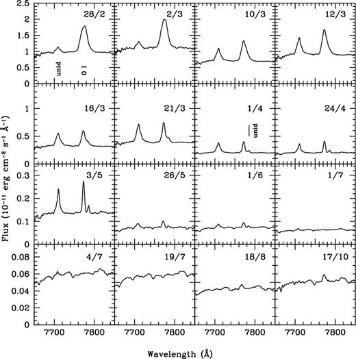
Evolution of the O i 7774 Å line (top to bottom, left to right). Dates are in the dd/mm format. The stronger line in the first panel (top left) is O i. On its left is the unidentified line at 7710 Å. The development of another unidentified line at 7785 Å can be seen (second panel from top). The O i line is seen to fade away in 2006 July, reappear in 2006 August and persist until 2006 October.
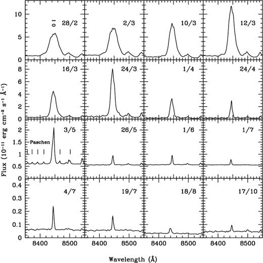
Evolution of the O i 8446 Å line (top to bottom, left to right). Dates are in the dd/mm format. The stronger line in all the panels is the O i line. Paschen lines can also be seen; they are narrow and clearly seen on 2006 May 3.
![Evolution of the [O iii] 4363 Å line (top to bottom, left to right). Dates are in the dd/mm format. Spectra in the last two columns in the first three rows have been scaled up for clarity. The strong line in the first panel (top left) is H γ. The 4363 Å line starts affecting the blue wing of H γ from 2006 March 16, and is clearly seen on 2006 April 1; it has almost disappeared by 2006 October 17.](https://oup.silverchair-cdn.com/oup/backfile/Content_public/Journal/mnras/474/3/10.1093_mnras_stx2988/2/m_stx2988fig10.jpeg?Expires=1749901161&Signature=l75aqrswwoYZSy916k0uvbr8Xw3vjHGA6ioV0eNqHjW6gTXYcvxi7BZrMGysDPxk2zSZPiJwZnjsSR8DoxHu9Gj2prT6Y6IQ6lQEQcYBE0-9nD1gY6j~ULwxkwKJy1y-YqUYmBnAwqRXJa9WiiINdA-W2BlajhMF9TW-5OqXw2Lkxbh6wgBJpI3xp8GapUCLFTHUCD9jFlUJh8LTgooeLtr5gx7y5FGWzPDUhQ7HhH3iZDhv5TPL~czhLuhxfSXR5UDnt8RWlvpTW4buyN-49X8-N6zew0K7SMjmCA1vYkSPiiOLfsyxb0ZPP-V1WrirQO-F~MdoOMQ5ixFFaCOmvA__&Key-Pair-Id=APKAIE5G5CRDK6RD3PGA)
Evolution of the [O iii] 4363 Å line (top to bottom, left to right). Dates are in the dd/mm format. Spectra in the last two columns in the first three rows have been scaled up for clarity. The strong line in the first panel (top left) is H γ. The 4363 Å line starts affecting the blue wing of H γ from 2006 March 16, and is clearly seen on 2006 April 1; it has almost disappeared by 2006 October 17.
![Evolution of the [O iii] 4959, 5007 Å lines (top to bottom, left to right). Dates are in the dd/mm format. Lines seen in the first panel (top left) belong to Fe ii; lines belonging to other species at similar wavelengths strengthen with time. By 2006 March 16, He i (the first two lines) has strengthened; the third (broad) line is mostly Si ii. The [O iii] 5007 line can be seen feebly on the blueward side of the He i 5016 line. The [O iii] 4959 and 5007 lines can be clearly seen in the spectrum obtained on 2006 May 3; they persist until 2006 October 17.](https://oup.silverchair-cdn.com/oup/backfile/Content_public/Journal/mnras/474/3/10.1093_mnras_stx2988/2/m_stx2988fig11.jpeg?Expires=1749901161&Signature=UE2JRs1Cz4oXsI2Ei5g09SzbyVW8t~swC7SA8UPbzHLPEtfa9on5XxqSIJcrclS5fT1ID3Kkr9ll~7vm8MwfY-1P4KyJo3JXhnlYzhWFcAhmurAqnsjJihZVF5WToF2VPMGk9hOC74ResMYFzIFT0N3E90NJSsBGxyAY3w4mXIEYE4MeL9TLQ1KLDfzZnHuRVGh6gX~1O~TZL-Za4rHywYeWGaP0ZMaURpGUX9qhG51WzyaybfpGK4g10Qe1MbmHEk4UrBLiMUEUBhkJtzjZ5eXBAHpbW9ZBIRsAMHjjlI1QgYThPy6NAWVwzouweG4bu47pbFTtzt3z0FS0MRZLLQ__&Key-Pair-Id=APKAIE5G5CRDK6RD3PGA)
Evolution of the [O iii] 4959, 5007 Å lines (top to bottom, left to right). Dates are in the dd/mm format. Lines seen in the first panel (top left) belong to Fe ii; lines belonging to other species at similar wavelengths strengthen with time. By 2006 March 16, He i (the first two lines) has strengthened; the third (broad) line is mostly Si ii. The [O iii] 5007 line can be seen feebly on the blueward side of the He i 5016 line. The [O iii] 4959 and 5007 lines can be clearly seen in the spectrum obtained on 2006 May 3; they persist until 2006 October 17.
4.3 Helium lines
There is only a hint of the He i 4471 Å line on 2006 February 13; it shows up clearly two days later. The 5876 Å line is very broad with a sharp central absorption on 2006 February 13. It has contributions from some other line on its redward side till 2006 April. On 2006 February 13, the 6678 Å line is very broad with a central absorption, which persists until early 2006 March. The 7065 Å line shows a central absorption on 2006 February 13 that shifts to the redward side on subsequent days. By 2006 March 16, the line has a Gaussian-like appearance. All the He i lines persist until 2006 October 17; the 7065 Å line shows a P Cygni profile from 2006 July onwards (see Fig. 12). The He ii 4686 Å line appears on 2006 February 27 with a narrower FWHM than the Balmer lines; emission lines at this position in earlier spectra are likely to be contributions from Fe ii. By 2006 March 10, its width is similar to H β. This line persists until 2006 October 17 (see Fig. 13).
Evolution of the He i 7065 Å line. Dates are in the dd/mm format.
Evolution of the He ii 4686 Å line (top to bottom, left to right). Dates are in the dd/mm format. Lines seen in the first panel (top left) belong to Fe ii and N iii (the strongest line). The strong, narrow He ii line is clearly seen by 2006 March 10 and persists till 2006 October 17.
4.4 Nitrogen lines
The [N ii] 5755 Å line is present from February 13. It is very broad initially but narrows down by February 15. The 5660 Å appears on February 16 and is broad, blended with the 5680 Å feature. From February 20 onwards it has a narrow component on top of a broad feature. Other nitrogen lines show up after February 26. The 5755 Å line has a triangular shape and is seen to narrow with time. It suddenly broadens on 26 May. This line persists until 2006 October 17 (see Fig. 14). The ‘4640’ complex is observed from 2006 February to 2006 October (see Fig. 13).
![Evolution of the [N ii] 5680 and 5755 Å lines (top to bottom, left to right). Dates are in the dd/mm format. Both the lines (5660 + 5680 blend and 5755) are seen in the first panel. The 5660/5680 line weakens and is replaced by the [Fe vi] 5679 line in later spectra. The [Fe vii] 5721 line shows as a small kink on the redward side of 5755 on 2006 March 16, becomes stronger and fades away by 2006 August 18.](https://oup.silverchair-cdn.com/oup/backfile/Content_public/Journal/mnras/474/3/10.1093_mnras_stx2988/2/m_stx2988fig14.jpeg?Expires=1749901161&Signature=pYAy2OHfe9tK0Trj4hTaZ4KvKQP4FDmu20zvhc3pkD53jf97uPmC14bFw2c~bjJ2CZyS7zu3kytJGkpnYBFm3eb78Tbi46PtET5JVOvxdrqM8kWlT-RJTAWJHOABjGkFIytROg1HxMQHGUHE5Zjo-APH0HQV~ltr81Ngl14U5sBVBOYfSgV~m4MQ2Sh7FAnk2yF5m8K-fmCEuh1vbPF24oNWJzSota8JWbLEE95MG3ruUyWBz9tr6Br7V1rTz1bY6sHH28lWIy4BEitowCjWTizL-pyUUQ5mf7kUR56Ykvwo-IU1k03aNtml0XF2B1zlFUHyNts7m80Vw0GBeW7Y~Q__&Key-Pair-Id=APKAIE5G5CRDK6RD3PGA)
Evolution of the [N ii] 5680 and 5755 Å lines (top to bottom, left to right). Dates are in the dd/mm format. Both the lines (5660 + 5680 blend and 5755) are seen in the first panel. The 5660/5680 line weakens and is replaced by the [Fe vi] 5679 line in later spectra. The [Fe vii] 5721 line shows as a small kink on the redward side of 5755 on 2006 March 16, becomes stronger and fades away by 2006 August 18.
4.5 Coronal lines
Coronal lines in RS Oph were first seen and identified by Adams & Joy (1933) on day 51 during the 1933 outburst. The presence of five coronal lines at 3987, 4086, 4231, 5303 and 6374 Å could be well established on their spectrograms obtained on later nights. In this outburst, coronal lines of neon ([Ne iii], [Ne v]), argon ([Ar iv], [Ar x], [Ar xi], [Ar xiv]) and iron ([Fe vii], [Fe x], [Fe xi], [Fe xiv]) can be clearly seen in the spectra obtained during 2006 March–June. It appears that the calcium lines showed an unusual behaviour during this outburst as compared to the previous outbursts. [Ca xiii] 4086 Å was absent; [Ca xv] 5694 Å was not prominent. The temporal development of the iron green and red coronal lines is shown in Figs 15 and 16, respectively. Many coronal lines are close in wavelength to other permitted or low ionization lines – for example, [Ne iii] 3970 Å and H ε, [Ni xii] 4231 Å and Fe ii, [Ar xiv] 4412 and [Fe ii], etc. – and it becomes difficult to separate the contributions from the individual components from observations of emission lines. However, it is very likely that the permitted or low ionization lines are the dominant contributors in the early outburst spectra.
![Evolution of the [Fe xiv] 5303 Å line (top to bottom, left to right). Dates are in the dd/mm format. Fe ii lines are seen in the first panel (top left). The [Fe xiv] appears as a small kink on the redward side of the Fe ii 5317 line on 2006 March 16, increasing in strength by 2006 May 3, and barely seen by 2006 June 1. The last row of spectra displays just the fluctuations at the continuum level.](https://oup.silverchair-cdn.com/oup/backfile/Content_public/Journal/mnras/474/3/10.1093_mnras_stx2988/2/m_stx2988fig15.jpeg?Expires=1749901161&Signature=V45Zm9v4pv5~WNM6UQrah7HuuORDwwei0yEeIbUvll5tUqcUCStK0sahj8iGYCOEO9bNhpj6fJz2ohK-SZJjkiELbu5VaBmHCEhKQiIC98Ro7B4Po0fK94Hi83IiNxltXM9i5jwUMY4GJrHOXES24fg9p~WML7fuFauhuyVuKS9Ty5rBgsC9eq2nezEACQQt9pieuZFxerqO3d4ozch-Oj0n058iRfhhvVz0RLSGO2OqvMti9jidkW-tFtJnApXTuR4XcwwLBxSezhSWzm-yEYet4Tct8zJ1Ef7SgwIHq3NBoQ4fYZfnMBaknD095VBtm18wgU31zk3-QSsrPHAX8Q__&Key-Pair-Id=APKAIE5G5CRDK6RD3PGA)
Evolution of the [Fe xiv] 5303 Å line (top to bottom, left to right). Dates are in the dd/mm format. Fe ii lines are seen in the first panel (top left). The [Fe xiv] appears as a small kink on the redward side of the Fe ii 5317 line on 2006 March 16, increasing in strength by 2006 May 3, and barely seen by 2006 June 1. The last row of spectra displays just the fluctuations at the continuum level.
![Evolution of the [Fe x] 6374 Å line (top to bottom, left to right). Dates are in the dd/mm format. The broad lines seen in the first panel (top left) are mostly Si ii. The [Fe x] 6374, [S iii] + [K v] 6315 are seen on 2006 March 10. The [O i] 6300 line is also feebly seen on this day. By 2006 August 18, only the [O i] 6300 and 6363 lines are clearly seen.](https://oup.silverchair-cdn.com/oup/backfile/Content_public/Journal/mnras/474/3/10.1093_mnras_stx2988/2/m_stx2988fig16.jpeg?Expires=1749901161&Signature=4QNeEBCuBJnnhPJkWdUCm~-Hi4BDlYpnRG21~yQY-2WdDXNorktvsOVXlQtt3D7JYUi4g5XhlerVm~YhrYAnPjYts0rJlAZJe4y~ojBClXJRMsGWqOCesPjl87JYSHcvTcU-lRQ9Uuooux-SXd2O5N1tBUmQoJxQOcoPP1edITq-BMgppNKhHJXM8dGuVA5~aCnH~LCWZQlUTh-0bV79rXX7ENDcfBdEp4Yx4-B62AY7OXPgpzdmNxwCZYe5QaMYvOPNPxNLG9k4~ETMhSjFU5BpZ3KWi5c3ls-kblKLrdB1tTnl4zZH-OAVUmJ2yeJTjfVEWWmZn9a5wC1ev03-BQ__&Key-Pair-Id=APKAIE5G5CRDK6RD3PGA)
Evolution of the [Fe x] 6374 Å line (top to bottom, left to right). Dates are in the dd/mm format. The broad lines seen in the first panel (top left) are mostly Si ii. The [Fe x] 6374, [S iii] + [K v] 6315 are seen on 2006 March 10. The [O i] 6300 line is also feebly seen on this day. By 2006 August 18, only the [O i] 6300 and 6363 lines are clearly seen.
4.6 The Raman-scattered 6830, 7088 Å lines
The strong line at 6830 Å that was first seen in the 1933 outburst was attributed to [Kr iii] (Joy & Swings 1945). This line was also seen in other outbursts. We now know that this emission feature, seen in many symbiotic stars, is due to the Raman scattering of the O vi 1032 Å line by neutral hydrogen (Schmid 1989). Schmid also noted that in some symbiotic stars a fainter companion feature appears at 7088 Å. This is due to the same process as for the 1038 Å line of the O vi resonance doublet. Schmid has suggested that this Raman scattering in symbiotic stars takes place in the atmosphere of the cool giant and in the inner parts of its stellar wind. The presence of the Raman-scattered O vi lines implies the existence of a hot ionizing source, the WD on which hydrogen is still burning after the outburst. The 2006 outburst is the first one since this identification was done. This line is first seen in our spectrum of 2006 March 10 and persists until 2006 August 18. In our next spectrum obtained on 2006 October 17, this line is probably not seen; other nearby lines dominate this wavelength region (see Fig. 17). The 7088 line is also feebly seen in the wings of He i 7065 Å during the same period.
![Evolution of the Raman-scattered 6830 Å line (top to bottom, left to right). Dates are in the dd/mm format. This line appears suddenly on 2006 March 10; there is no gradual strengthening as seen for other lines. It disappears after 2006 July 19. The [Ar xi] 6919 line is seen during 2006 March 16 to 2006 May 3.](https://oup.silverchair-cdn.com/oup/backfile/Content_public/Journal/mnras/474/3/10.1093_mnras_stx2988/2/m_stx2988fig17.jpeg?Expires=1749901161&Signature=vCki-ST4Bsr5HQYKWyonHZAasCNIYVXz2upRMTv2QCdV7JzLrF5WgWGuDHi6kVB~K01AIyKA7besaZoinY12uw6wxoVxpw2Q9a3gDTFCFRebmYaTyyuYxu4eWXIBV1EqwshOnTW1M480OE~vFklbGzAATl8B-gFAB0YCFYfblGe9fu525Dw~dWG97yuakhzXaqL1cmgt9tqXUPNrPiz42UJSW2DySbfhGn1jW96VMlxEDu-e0sJ8Yl-YR1f9kaALgudkeWj33X1oHp6LISqtIQ7Cr~cjlpsEacKq1e7b~X2ej7wlZ5wS9W-yMNOOqWci8MzIjgc-U8wIUrJ7yirhGg__&Key-Pair-Id=APKAIE5G5CRDK6RD3PGA)
Evolution of the Raman-scattered 6830 Å line (top to bottom, left to right). Dates are in the dd/mm format. This line appears suddenly on 2006 March 10; there is no gradual strengthening as seen for other lines. It disappears after 2006 July 19. The [Ar xi] 6919 line is seen during 2006 March 16 to 2006 May 3.
4.7 Formation of the spectral lines
Swift observations have revealed the existence of a supersoft X-ray phase during days 26–90 of the outburst, which is due to the matter burning quiescently on the WD (Osborne et al. 2011). This source peaks at around day 50, similar to the behaviour of the coronal lines. This indicates that some of the flux in the coronal lines, especially during days 26–90, must be due to photoionization. As mentioned in Section 4.6, the behaviour of the Raman lines also corroborates this idea. The He ii and O iv lines with high ionization potentials were also strong during 2006 March–June. Similarly, multi-frequency radio data show that the spectral index is consistent with a mixed non-thermal and thermal emission during days 5–60 (Eyres et al. 2009). Therefore, as for other novae, optical spectra should show the characteristics of photoionized ejecta. Photoionization could even be the dominant mechanism, at least during days 29–90. So, in Section 5, we attempt the photoionization modelling of our optical spectra using cloudy.
5 PHOTOIONIZATION MODEL ANALYSIS
6 RESULTS AND DISCUSSIONS
6.1 Early phase: 2006 February–May
Relative fluxes of the best-fitting model-predicted lines, observed lines and corresponding χ2 values during the early phase are presented in Table 2. Here, we have considered the lines that are present both in the model-generated and observed spectra for the calculation of χ2 values. The observed line fluxes have been determined using iraf tasks; the profiles that have multiple components have been decomposed with multiple Gaussians using iraf tasks. To minimize errors associated with flux calibration between different epochs, the modelled and observed flux ratios have been calculated relative to H β. The values of the best-fitting parameters are presented in Table 4. The best-fitting modelled spectra (grey lines) with the observed optical spectra (black lines) during this phase are shown in Figs 18 –22. The spectra, in the early phase, are dominated by prominent features of low ionization lines, e.g. H ε (3970 Å), H δ (4101 Å), H γ (4340 Å), He ii (4686 Å), H β (4863 Å). There are also some higher ionization lines, e.g. [Fe vii] (3760 Å), Fe ii and [Ni xii] (4233 Å), He i and [Ar iv] (4713 Å), [Ar x] (5535 Å), [Fe xi] (7890 Å), [Fe x] (6374 Å), [Fe xiv] (5303 Å) etc., which start to appear at the end of the early phase. Since the gas is highly inhomogeneous at this time, a one-component model was unable to fit the H α/H β flux ratio properly. So, we had to consider a two-component model. The first component (clump) consisted of a highly dense cloud to fit the lower ionization lines. This component was optically thick, and Case-B was taken into consideration as well. The majority of the observed lines were generated using this component, but it under-represents the highest ionization lines. The second component (diffuse), with a lower density, was smaller (10–30 per cent) in volume, but it allowed the source photon to ionize some of the species to their higher ionization states (e.g. [Ar iv] (4713 Å), [Ar x] (5535 Å)), while not changing the clump contribution to the spectra.

Best-fitting cloudy model spectra (grey line) plotted over the observed spectra (black lines) of RS Oph observed on 2006 February 21. The spectra were normalized to H β. A few of the strong features have been marked (see text for details).
Best-fitting cloudy model spectra (grey line) plotted over the observed spectra (black lines) of RS Oph observed on 2006 February 24. The spectra were normalized to H β. A few of the strong features have been marked (see text for details).
Best-fitting cloudy model spectra (grey line) plotted over the observed spectra (black lines) of RS Oph observed on 2006 March 12. The spectra were normalized to H β. A few of the strong features have been marked (see text for details).

Best-fitting cloudy model spectra (grey line) plotted over the observed spectra (black lines) of RS Oph observed on 2006 April 3. The spectra were normalized to H β. A few of the strong features have been marked (see text for details).
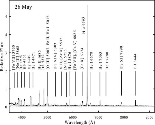
Best-fitting cloudy model spectra (grey line) plotted over the observed spectra (black lines) of RS Oph observed on 2006 May 26. The spectra were normalized to H β. A few of the strong features have been marked (see text for details).
Observed and best-fitting cloudy model line fluxes.
| λ | Feb 21 | Feb 24 | Mar 12 | Apr 3 | May 26 | |||||||||||
|---|---|---|---|---|---|---|---|---|---|---|---|---|---|---|---|---|
| (Å) | Line | Obs. | Mod. | χ2 | Obs. | Mod. | χ2 | Obs. | Mod. | χ2 | Obs. | Mod. | χ2 | Obs. | Mod. | χ2 |
| 3750 | H12 | 0.04 | 0.04 | 0.00 | 0.02 | 0.05 | 0.09 | – | – | – | – | – | – | – | – | – |
| 3760 | [Fe vii] | – | – | – | – | – | – | – | – | – | 0.07 | 0.19 | 1.62 | 0.31 | 0.14 | 2.85 |
| 3771 | H11 | 0.06 | 0.01 | 0.22 | 0.03 | 0.04 | 0.00 | – | – | – | – | – | – | 0.03 | 0.05 | 0.06 |
| 3798 | H10 | 0.10 | 0.06 | 0.18 | 0.06 | 0.06 | 0.00 | 0.03 | 0.07 | 0.17 | 0.07 | 0.06 | 0.02 | 0.08 | 0.10 | 0.08 |
| 3835 | H η | 0.18 | 0.07 | 1.17 | 0.14 | 0.17 | 0.08 | 0.04 | 0.12 | 0.61 | 0.10 | 0.14 | 0.21 | 0.13 | 0.13 | 0.0 |
| 3868 | [Ne iii] | – | – | – | – | – | – | – | – | – | 0.20 | 0.14 | 0.42 | 0.62 | 0.49 | 1.67 |
| 3889 | H ζ, He i | 0.27 | 0.14 | 1.82 | 0.22 | 0.20 | 0.06 | 0.12 | 0.15 | 0.10 | 0.26 | 0.29 | 0.10 | 0.38 | 0.29 | 0.7 |
| 3970 | H ε, [Ne iii] | 0.26 | 0.21 | 0.29 | 0.18 | 0.13 | 0.26 | 0.12 | 0.16 | 0.30 | 0.26 | 0.19 | 0.46 | 0.36 | 0.21 | 2.22 |
| 4026 | He i, He ii | 0.05 | 0.03 | 0.04 | 0.05 | 0.03 | 0.06 | 0.04 | 0.06 | 0.04 | 0.05 | 0.06 | 0.02 | 0.05 | 0.06 | 1.83 |
| 4070 | [S ii] | – | – | – | – | – | – | – | – | – | – | – | – | 0.10 | 0.03 | 0.55 |
| 4101 | H δ | 0.34 | 0.32 | 0.02 | 0.28 | 0.29 | 0.02 | 0.22 | 0.19 | 0.09 | 0.33 | 0.33 | 0.0 | 0.05 | 0.28 | 0.48 |
| 4144 | He i | – | – | – | – | – | – | – | – | – | – | – | – | 0.03 | 0.02 | 0.02 |
| 4180 | Fe ii, [Fe ii] | – | – | – | – | – | – | – | – | – | 0.05 | 0.02 | 0.10 | 0.06 | 0.03 | 0.09 |
| 4233 | Fe ii, [Ni xii] | 0.05 | 0.06 | 0.00 | 0.03 | 0.04 | 0.00 | 0.03 | 0.03 | 0.00 | 0.06 | 0.04 | 0.03 | 0.07 | 0.05 | 0.04 |
| 4242 | N ii | – | – | – | – | – | – | – | – | – | 0.02 | 0.04 | 0.05 | 0.09 | 0.07 | 0.05 |
| 4340 | H γ | 0.45 | 0.22 | 5.33 | 0.39 | 0.33 | 0.29 | 0.30 | 0.34 | 0.19 | 0.34 | 0.29 | 0.22 | 0.52 | 0.40 | 1.38 |
| 4415 | [Fe ii] | – | – | – | – | – | – | – | – | – | 0.04 | 0.04 | 0.00 | 0.06 | 0.07 | 0.00 |
| 4471 | He i | 0.11 | 0.07 | 0.12 | 0.09 | 0.06 | 0.10 | 0.05 | 0.11 | 0.44 | 0.06 | 0.09 | 0.14 | 0.11 | 0.12 | 0.00 |
| 4584 | Fe ii | – | – | – | – | – | – | 0.03 | 0.03 | 0.00 | 0.04 | 0.05 | 0.02 | – | – | – |
| 4686 | He ii | – | – | – | – | – | – | 0.34 | 0.19 | 2.22 | 0.52 | 0.37 | 1.9 | 0.65 | 0.52 | 1.82 |
| 4713 | He i, [Ar iv] | – | – | – | 0.04 | 0.03 | 0.00 | 0.02 | 0.01 | 0.03 | 0.21 | 0.07 | 1.9 | – | – | – |
| 4863 | H β | 1.00 | 1.00 | 0.00 | 1.00 | 1.00 | 0.00 | 1.00 | 1.00 | 0.00 | 1.00 | 1.00 | 0.00 | 1.00 | 1.00 | 0.00 |
| 4922 | Fe ii, He i | 0.09 | 0.05 | 0.19 | 0.09 | 0.06 | 0.06 | 0.07 | 0.06 | 0.01 | 0.06 | 0.04 | 0.05 | 0.09 | 0.11 | 0.04 |
| 4959 | [O iii] | – | – | – | – | – | – | – | – | – | 0.06 | 0.05 | 0.00 | 0.46 | 0.31 | 2.15 |
| 5007 | [O iii] | – | – | – | – | – | – | – | – | – | 0.23 | 0.14 | 0.84 | 1.06 | 0.01 | 0.23 |
| 5016 | Fe ii, He i | 0.15 | 0.08 | 0.43 | 0.18 | 0.07 | 1.16 | – | – | – | – | – | – | – | – | – |
| 5169 | Fe ii | 0.08 | 0.13 | 0.28 | 0.09 | 0.08 | 0.01 | – | – | – | – | – | – | – | – | – |
| 5235 | Fe ii | 0.02 | 0.18 | 2.57 | 0.02 | 0.01 | 0.01 | – | – | – | – | – | – | – | – | – |
| 5276 | Fe ii | 0.03 | 0.08 | 0.29 | 0.03 | 0.06 | 0.08 | – | – | – | – | – | – | – | – | – |
| 5303 | [Fe xiv] | – | – | – | – | – | – | – | – | – | 0.10 | 0.09 | 0.02 | – | – | – |
| 5317 | Fe ii | 0.05 | 0.04 | 0.02 | 0.04 | 0.03 | 0.00 | – | – | – | – | – | – | – | – | – |
| 5412 | He ii | – | – | – | – | – | – | – | – | – | 0.06 | 0.10 | 0.19 | 0.09 | 0.09 | 0.00 |
| 5535 | N ii, [Ar x] | – | – | – | – | – | – | 0.02 | 0.02 | 0.00 | 0.09 | 0.02 | 0.47 | 0.08 | 0.04 | 0.15 |
| 5755 | [N ii] | – | – | – | – | – | – | – | – | – | 0.07 | 0.04 | 0.12 | 0.43 | 0.32 | 1.26 |
| 5876 | He i | 0.31 | 0.30 | 0.00 | 0.44 | 0.24 | 3.98 | 0.50 | 0.46 | 0.16 | 0.29 | 0.34 | 0.28 | 0.29 | 0.43 | .89 |
| 6086 | [Fe vii], [Ca v] | – | – | – | – | – | – | – | – | – | – | – | – | 0.20 | 0.32 | 1.55 |
| 6101 | O iv | – | – | – | – | – | – | 0.03 | 0.03 | 0.00 | – | – | – | – | – | – |
| 6300 | [O i] | – | – | – | – | – | – | – | – | – | – | – | – | 0.12 | 0.18 | 0.37 |
| 6374 | [Fe x] | – | – | – | – | – | – | – | – | – | 0.32 | 0.07 | 6.27 | 0.33 | 0.29 | 0.16 |
| 6563 | H α | 4.74 | 4.45 | 8.26 | 6.12 | 5.76 | 12.53 | 9.60 | 9.24 | 12.72 | 5.81 | 6.15 | 12.08 | 4.46 | 4.75 | 8.83 |
| 6678 | He i | 0.09 | 0.08 | 0.02 | 0.14 | 0.06 | 0.64 | 0.17 | 0.12 | 0.23 | 0.08 | 0.1 | 4.62 | 0.12 | 0.12 | 0.00 |
| 6830 | Raman | – | – | – | – | – | – | 0.03 | 0.01 | 0.03 | – | – | – | – | – | – |
| 7065 | He i | 0.14 | 0.16 | 0.02 | 0.24 | 0.16 | 0.63 | 0.37 | 0.35 | 0.03 | 0.19 | 0.27 | 0.65 | 0.21 | 0.37 | 0.67 |
| 7280 | He i | 0.03 | 0.08 | 0.23 | 0.07 | 0.06 | 0.00 | 0.03 | 0.04 | 0.01 | 0.02 | 0.04 | 0.05 | 0.02 | 0.05 | 0.13 |
| 7890 | [Fe xi] | – | – | – | – | – | – | – | – | – | 0.15 | 0.02 | 1.65 | 0.16 | 0.06 | 0.96 |
| 8598 | Pa14 | 0.03 | 0.04 | 0.00 | 0.04 | 0.03 | 0.00 | 0.05 | 0.03 | 0.05 | 0.02 | 0.02 | 0.0 | 0.02 | 0.03 | 0.02 |
| 8750 | Pa12 | 0.04 | 0.03 | 0.00 | 0.06 | 0.06 | 0.00 | 0.07 | 0.04 | 0.07 | 0.03 | 0.03 | 0.0 | 0.02 | 0.03 | 0.02 |
| 8862 | Pa11 | 0.06 | 0.04 | 0.03 | 0.08 | 0.04 | 0.13 | 0.09 | 0.06 | 0.09 | 0.03 | 0.03 | 0.0 | 0.02 | 0.03 | 0.03 |
| 9015 | Pa10 | 0.09 | 0.10 | 0.02 | 0.09 | 0.11 | 0.03 | 0.12 | 0.09 | 0.09 | 0.03 | 0.06 | 0.09 | 0.01 | 0.07 | 0.42 |
| Total | – | – | 21.60 | – | – | 20.28 | – | – | 17.71 | – | – | 30.49 | – | – | 32.94 |
Initially, in 2006 February, the ionizing source is surrounded by a dense (nH ∼ 1011 cm−3) cloud. So, the effective temperature and luminosity (T ∼ 104.45 K, L ∼ 1036.8 erg s−1) of the source is relatively lower. As the ejecta expands, more energy from the central engine comes out. Therefore, while the ejecta density decreases (nH ∼ 108.41 cm−3), the blackbody temperature (TBB) and the luminosity increases to TBB ∼ 105.6 K and L ∼1037.1 erg s−1, respectively, in 2006 May to photoionize more matter. The estimated elemental abundances during this phase are given as logarithms of the numbers relative to hydrogen and relative to solar values in Table 4. The values show that the helium, nitrogen, oxygen, neon, argon, iron and nickel abundances are all enhanced relative to solar values whereas the abundances of calcium and sulfur are at solar values. However, we must be cautious while considering the abundances of calcium, because calcium abundance was calculated using only the Ca v (6086 Å) line observed on 2006 May 26. This line is blended with [Fe vii]. So, first, the iron abundance was set using the other prominent Fe ii (4180 Å, 4415 Å and 4584 Å) lines. Then, the calcium abundance was changed such that the total flux of the blended feature in the model matched the observed spectra. Similarly, the nitrogen abundance on day 28 was determined using the N ii (5535 Å) line blended with [Ar x]. But, on days 50 and 103, there are two other N ii (4242 Å and 5755 Å) lines that helped to set the nitrogen abundance correctly. These values match the results obtained by Das & Mondal (2015).
6.2 Nebular phase: 2006 July–October
The prominent appearance of higher ionization lines like [O iii](4363, 4959, 5007 Å) and [O i] (6300 Å) in the day 103 spectrum indicates that the nova is entering the nebular phase. Due to the expansion of the shell, the cloud becomes thinner and consequently higher ionization lines are seen in the spectra. Modelling of the nebular phase was simpler as only one component of relatively lower hydrogen density was sufficient to generate the high as well as the low ionization emission lines observed in the spectra. The line fluxes and χ2 values are presented in Table 3 and the best-fitting model parameters are presented in Table 4. During this phase, the effective temperature and luminosity were increased to 105.95 K and 1037.5 ergs s−1, respectively, and the hydrogen density was decreased to 107.18 cm−3 to match the observed spectra. The estimated value of temperature is in agreement with the WD temperature of around 8 × 10⁵ K derived from X-ray studies (Nelson et al. 2008). During the early phase, we have seen that the abundances of several elements were enhanced relative to solar values, but as the nebular phase set in, the oxygen, neon and iron abundances become subsolar, whereas the sulfur abundance is enhanced from the solar abundance seen in the early phase. Also in the nebular phase, the calcium abundance, which was at a solar value, was calculated using only the blended Ca v (6086 Å) line. However, the nitrogen abundance was determined correctly as the prominent [N ii] (5755 Å) line is highly sensitive to the change in abundance parameter in cloudy. The best-fitting modelled spectra (grey lines) with the observed optical spectra (black lines) during this phase are shown in Figs 23 –25.
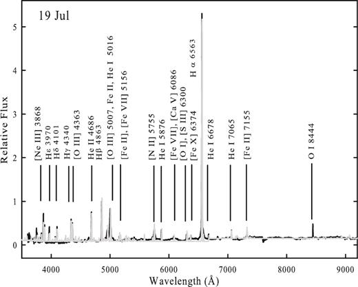
Best-fitting cloudy model spectra (grey line) plotted over the observed spectra (black lines) of RS Oph observed on 2006 July 19. The spectra were normalized to H β. A few of the strong features have been marked (see text for details).
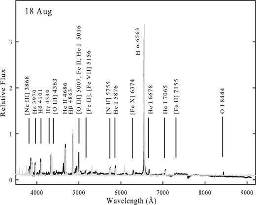
Best-fitting cloudy model spectra (grey line) plotted over the observed spectra (black lines) of RS Oph observed on 2006 August 18. The spectra were normalized to H β. A few of the strong features have been marked (see text for details).
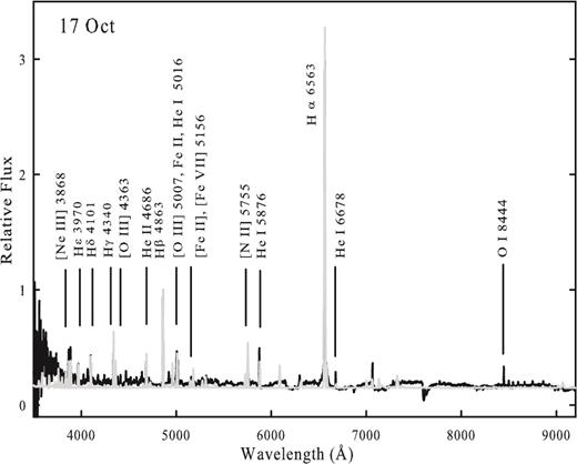
Best-fitting cloudy model spectra (grey line) plotted over the observed spectra (black lines) of RS Oph observed on 2006 October 17. The spectra were normalized to H β. A few of the strong features have been marked (see text for details).
Observed and best-fitting cloudy model line fluxes.
| λ | Jul 19 | Aug 18 | Oct 17 | |||||||
|---|---|---|---|---|---|---|---|---|---|---|
| (Å) | Line | Obs. | Mod. | χ2 | Obs. | Mod. | χ2 | Obs. | Mod. | χ2 |
| 3868 | [Ne iii] | 0.80 | 0.65 | 1.00 | 0.44 | 0.51 | 0.22 | 0.30 | 0.54 | 2.56 |
| 3889 | H ζ, He i | 0.38 | 0.29 | 0.36 | 0.26 | 0.18 | 0.28 | 0.28 | 0.20 | 028 |
| 3970 | H ε, [Ne iii] | 0.43 | 0.31 | 0.64 | 0.37 | 0.19 | 1.44 | 0.30 | 0.18 | 0.64 |
| 4026 | He i, He ii | 0.09 | 0.04 | 0.11 | 0.08 | 0.02 | 0.16 | 0.08 | 0.02 | 0.16 |
| 4101 | H δ | 0.38 | 0.28 | 0.44 | 0.43 | 0.28 | 1.0 0 | 0.31 | 0.27 | 0.07 |
| 4180 | Fe ii, [Fe ii] | 0.06 | 0.02 | 0.07 | 0.09 | 0.01 | 0.28 | – | – | – |
| 4244 | [Fe ii] | 0.12 | 0.10 | 0.02 | 0.16 | 0.02 | 0.87 | 0.23 | 0.02 | 1.96 |
| 4340 | H γ | 0.56 | 0.46 | 0.44 | 0.49 | 0.49 | 0.00 | 0.34 | 0.43 | 0.36 |
| 4363 | [O iii] | 0.72 | 0.54 | 1.44 | 0.31 | 0.32 | 0.00 | 0.09 | 0.05 | 0.07 |
| 4415 | [Fe ii] | 0.09 | 0.08 | 0.00 | 0.08 | 0.01 | 0.22 | 0.14 | 0.02 | 0.64 |
| 4471 | He i | 0.08 | 0.09 | 0.00 | 0.11 | 0.08 | 0.04 | 0.14 | 0.04 | 0.44 |
| 4686 | He ii | 0.65 | 0.66 | 0.00 | 0.62 | 0.60 | 0.02 | 0.29 | 0.50 | 1.96 |
| 4863 | H β | 1.00 | 1.00 | 0.00 | 1.00 | 1.00 | 0.00 | 1.00 | 1.00 | 0.00 |
| 4922 | Fe ii, He i | 0.10 | 0.0 | 0.28 | 0.14 | 0.02 | 0.64 | 0.13 | 0.01 | 0.64 |
| 4959 | [O iii] | 0.94 | 0.89 | 3.00 | 0.45 | 0.37 | 0.28 | 0.19 | 0.22 | 0.04 |
| 5007 | [O iii], Fe ii, He i | 2.00 | 1.62 | 6.42 | 1.18 | 0.82 | 5.76 | 0.89 | 0.67 | 2.15 |
| 5156 | [Fe ii], [Fe vii] | 0.13 | 0.08 | 0.11 | 0.13 | 0.02 | 0.54 | 0.12 | 0.02 | 0.44 |
| 5755 | [N ii] | 0.35 | 0.41 | 0.16 | 0.12 | 0.15 | 0.04 | 0.38 | 0.40 | 0.02 |
| 5876 | He i | 0.28 | 0.30 | 0.02 | 0.25 | 0.15 | 0.44 | 0.43 | 0.23 | 0.54 |
| 6086 | [Fe vii], [Ca v] | 0.13 | 0.30 | 1.28 | – | – | – | – | – | – |
| 6300 | [O i], [S iii] | 0.26 | 0.48 | 2.15 | – | – | – | 0.15 | 0.04 | 0.54 |
| 6374 | [Fe x] | 0.17 | 0.02 | 1.0 | 0.21 | 0.04 | 1.28 | – | – | – |
| 6563 | H α | 5.12 | 5.21 | 0.36 | 3.61 | 3.73 | 0.64 | 4.03 | 4.06 | 0.04 |
| 6678 | He i | 0.11 | 0.07 | 0.07 | 0.13 | 0.03 | 0.44 | 0.13 | 0.03 | 0.4 |
| 7065 | He i | 0.16 | 0.18 | 0.02 | 0.14 | 0.10 | 0.07 | – | – | – |
| 7155 | [Fe ii] | 0.05 | 0.02 | 0.02 | 0.03 | 0.02 | 0.00 | – | – | – |
| Total | – | – | 19.44 | – | – | 14.69 | – | – | 15.24 |
Best-fitting cloudy model parameters during outburst phase (2006).
| Parameters | Feb | Feb | Mar | Apr | May | Jul | Aug | Oct |
|---|---|---|---|---|---|---|---|---|
| 21 | 24 | 12 | 3 | 26 | 19 | 18 | 17 | |
| (D9)a | (D12) | (D28) | (D50) | (D103) | (D159) | (D189) | (D249) | |
| Log(TBB) (K) | 4.45 | 4.5 | 5.0 | 5.5 | 5.6 | 5.8 | 5.9 | 5.95 |
| Log(luminosity) (erg s−1) | 36.9 | 36.8 | 37 | 37 | 37.1 | 37 | 37.5 | 37.3 |
| Log(Hden) (cm−3) | – | – | – | – | – | 7.74 | 7.61 | 7.18 |
| Log(Hden)[clump] (cm−3) | 11.0 | 10.8 | 9.5 | 8.8 | 8.5 | – | – | – |
| Log(Hden)[diffuse] (cm−3) | 10.5 | 9.8 | 8.2 | 8.0 | 7.6 | – | – | – |
| Clump-to-diffuse covering factor | 70/30 | 70/30 | 80/20 | 85/15 | 90/10 | – | – | – |
| αb | −3 | −3 | −3 | −3 | −3 | −3 | −3 | −3 |
| Log(Rin) (cm) | 13.94 | 14.01 | 14.28 | 14.45 | 14.71 | 15.0 | 15.1 | 15.28 |
| Log(Rout) (cm) | 14.26 | 14.33 | 14.63 | 14.83 | 15.13 | 15.3 | 15.4 | 15.6 |
| Filling factor | 0.1 | 0.1 | 0.1 | 0.1 | 0.1 | 0.1 | 0.1 | 0.1 |
| βc | 0.0 | 0.0 | 0.0 | 0.0 | 0.0 | 0.0 | 0.0 | 0.0 |
| He/He|$_{\odot }^{d}$| | 1.7(9) | 1.75(10) | 1.8(10) | 1.9(11) | 2.5(11) | 2.0(8) | 1.6(8) | 1.6(6) |
| N/N⊙ | – | – | 11.0(1) | 12(3) | 10(3) | 5.0(1) | 8.0(1) | 3.0(1) |
| O/O⊙ | – | – | 1.0(1) | 1.0(2) | 5(3) | 0.7(5) | 0.3(4) | 0.3(4) |
| Ne/Ne⊙ | 1.9(1) | 2.0(1) | 2.0(1) | 2.5(2) | 5(3) | 1.0(2) | 0.7(2) | 0.5(2) |
| Ar/Ar⊙ | – | 4.0(1) | 4.9(2) | 5.2(2) | 5.5(1) | – | – | – |
| Fe/Fe⊙ | 2.7(7) | 2.8(7) | 3.0(4) | 3.5(9) | 3.8(8) | 0.5(9) | 0.5(8) | 0.5(6) |
| Ca/Ca⊙ | – | – | – | – | 1.0(1) | 1.0(1) | – | – |
| S/S⊙ | – | – | – | – | 1.0(1) | 1.5(1) | – | 1.5(1) |
| Ni/Ni⊙ | 1.5(1) | 1.8(1) | 2.0(1) | 2.0(1) | 2.0(1) | – | – | – |
| CaseB–τ value | 4.8 | 4.2 | – | – | – | – | – | – |
| Number of observed lines (n) | 27 | 28 | 26 | 36 | 38 | 26 | 24 | 21 |
| Number of free parameters (np) | 9 | 10 | 12 | 12 | 14 | 11 | 10 | 10 |
| Degrees of freedom (ν) | 18 | 18 | 14 | 24 | 24 | 15 | 14 | 11 |
| Total χ2 | 21.60 | 20.28 | 17.71 | 30.49 | 32.94 | 19.44 | 14.69 | 15.24 |
| |$\chi ^{2}_{\rm red}$| | 1.2 | 1.13 | 1.26 | 1.27 | 1.37 | 1.29 | 1.05 | 1.39 |
Notes.aTime elapsed after discovery (in days)
bRadial dependence of the density rα
cRadial dependence of filling factor rβ
dAbundances are given on a logarithmic scale, relative to hydrogen. All other elements that are not listed in the table were set to their solar values. The number in parentheses represents the number of lines used in determining each abundance.
6.3 Quiescent phase
On October 17, around ∼250 d after the 2006 nova outburst, the spectrum shows a red continuum with clear TiO absorption bands at 4762, 5448, 5598, 5629 and 6159 Å. The absorption band indices indicate the secondary spectral type to be M2–M3. By this day the nebular line strengths have decreased. The Fe ii permitted lines normally seen in quiescence begin to appear. A year later, in 2007 April, when the nova reached quiescence, the continuum is bluer compared to the day ∼250 spectrum, indicating the presence of an accretion disc. The quiescent-phase spectrum shows prominent emission lines of H and He i, together with strong TiO absorption features that indicate the dominance of the secondary in the spectrum.
The elemental abundances during the quiescent period were estimated by photoionization modelling of the spectrum observed on 2007 April 26. To generate the model spectrum, three components were considered: a WD (T = 104.2 K) as an ionizing source, a cylindrical accretion disc (semi height =108 cm) surrounding the source and the secondary red giant of spectral type M2 III (Worters et al. 2007 and Anupama & Mikolajewska 1999). The final spectrum was obtained by adding the fluxes generated by these three components. The relative fluxes of the best-fitting model-predicted lines, observed lines and corresponding χ2 values during the quiescent period are presented in Table 5, and the best-fitting model parameters are presented in Table 6. The best-fitting parameters lead us to an accretion disc of low temperature (104.2 K) and low luminosity (1033 ergs s−1, and a luminosity of 1035 ergs s−1 for the red giant). As the dense H-rich material is accreted to the disc, the hydrogen density of the disc (1011 cm−3) is ∼10 times higher than that in the red giant (1010 cm−3). The Rin and Rout of the disc are calculated considering a high-mass WD of 1.35 M⊙ (e.g. Kato, Hachisu & Luna 2008). During the quiescent phase, the observed spectrum shows prominent H and He lines only. The estimated abundance of helium is 0.8, which is subsolar. Since there were no prominent lines of other elements, the abundances of other elements could not be estimated. The best-fitting modelled spectrum (grey lines), along with the observed optical spectrum (black lines) during this phase, is shown in Fig. 26.
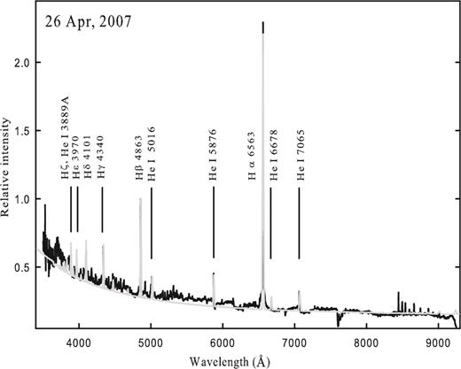
Best-fitting cloudy model spectra (grey line) plotted over the quiescent-phase spectra (black line) of RS Oph observed on 2007 April 26. The spectra were normalized to H β. A few of the strong features have been marked (see text for details).
Observed and best-fitting cloudy model line fluxes on 2007 Apr 26 (D438).
| λ | 26 Apr 2007 | |||
|---|---|---|---|---|
| (Å) | Line | Obs. | Mod. | χ2 |
| 3889 | H ζ, He i | 0.23 | 0.27 | 0.16 |
| 3970 | H η | 0.20 | 0.22 | 0.04 |
| 4101 | H δ | 0.38 | 0.35 | 0.11 |
| 4340 | H γ | 0.34 | 0.38 | 0.13 |
| 4863 | H β | 1.00 | 1.00 | 0.00 |
| 5016 | He i | 0.27 | 0.25 | 0.01 |
| 5876 | He i | 0.45 | 0.39 | 0.36 |
| 6563 | H α | 3.60 | 3.47 | 1.72 |
| 6670 | He i | 0.13 | 0.19 | 0.36 |
| 7065 | He i | 0.18 | 0.20 | 0.01 |
| Total | – | – | 2.89 |
Best-fitting cloudy model parameters during the quiescent phase.
| Parameters | Acc. disc (35 per cent)/ |
|---|---|
| red giant (65 per cent) | |
| Log(TBB) (K) | 4.2/4.2 |
| Log(luminosity) (erg s−1) | 33/35 |
| Log(Hden) (cm−3) | 11/10 |
| αa | −3/−3 |
| Log(Rin) (cm) | 9/12 |
| Log(Rout) (cm) | 11/15 |
| Filling factor | 0.1/0.1 |
| βb | 0.0/0.0 |
| He/He|$_{\odot }^{c}$| | 0.8(4)/0.8(4) |
| Number of observed lines (n) | 10 |
| Number of free parameters (np) | 8 |
| Degrees of freedom (ν) | 2 |
| Total χ2 | 2.89 |
| |$\chi ^{2}_{\rm red}$| | 1.44 |
Notes.aRadial dependence of the density rα
bRadial dependence of filling factor rβ
cAbundances are given on a logarithmic scale, relative to hydrogen. All other elements that are not listed in the table were set to their solar values. The number in parentheses represents the number of lines used in determining each abundance.
6.4 Comments on the models
Low values of |$\chi ^{2} _{\rm red}$| (between 1.05 to 1.44) indicate that the model-generated spectra match the observed ones well. However, in spite of the low |$\chi ^{2} _{\rm red}$| values, there are a few discrepancies. An inspection of Tables 2 and 3 shows that the χ2 values of some lines are relatively higher. For example, H α (6563 Å) in most of the epochs and H γ (4340 Å) on 2006 February 21 are the highest contributors to the χ2 values. Hence, the total χ2 value increases when these two strong lines are considered. Also, while adding the two components, emphasis was given to minimizing the total χ2 value, which leads to difficulty in matching the line flux ratios perfectly to the observed one. This problem disappears during the nebular-phase spectral modelling, where only one component of hydrogen density was enough to fit all the lines. The other lines that contribute to higher χ2 values are [Fe x] (6374 Å) and He i (6678 Å) on 2006 April 3. This is not surprising since [Fe x] is a coronal line, most likely excited by the shock interaction. The He i line is suppressed due to a high optical depth, which is not well accounted for in the model. The He ii line at 4686 Å in the modelled spectrum was weak on February 21 and 24. This is possibly because the temperature of the source on those two epochs (104.45 and 104.5 K, respectively) was low. A higher temperature ≳ 104.7 K is required to generate the He ii line (ionization potential ∼54.4 eV) prominently, as seen in the spectra of March 12 onwards, when the central source temperature was ≳ 105 K. Further, the He ii 4686 line was very weak in the observed spectra on those two epochs, and it was difficult to measure the flux correctly. Therefore, the He ii feature was not included in the calculation of the total χ2 for those epochs. In spite of the discrepancies, these fits do minimize the total χ2 values. During the nebular phases, the highest contributions to the total χ2 are due to the blending of [O iii], Fe ii and He i lines at 5007 Å. Also, the abundances for Fe, He and O were set after matching the other Fe, He and O lines, which leads to a high (about 30–40 per cent) χ2 contribution. Additionally, the model could not generate a few of the observed lines, e.g. N iii (4640 Å), Si ii (5041, 5056 Å), Ca ii (8668, 8548 Å), O i (7774, 8446 Å) and O vi (6106 Å). Some of these issues have been reported in our previous cloudy analysis of RS Oph spectra (Das & Mondal 2015). So, these lines have been excluded while calculating the values of χ2. This is possibly the reason that even a two-component model cannot properly represent the complex density structure of the nova ejecta.
7 SUMMARY
This is the first outburst of RS Oph that has revealed the complexity of emission mechanisms. This has been possible only due to the wide spectral and temporal coverage of the observations.
The evolution of the optical spectrum is very similar to previous outbursts.
The emission line velocity evolution indicates that the remnant was in the adiabatic phase for a very brief period and quickly moved to the radiative cooling phase by t ∼ 5 d. The nova remnant probably reached the edge of the red giant wind by ∼80 d, as indicated by the marginal increase in the emission line velocity. These findings are consistent with those based on X-ray observations (Bode et al. 2006).
The nebular lines originate in a region closer to the WD while the recombination lines originate in the decelerating material.
The observed spectra are modelled using the photoionization code cloudy for 9 epochs. Based on the modelling, the elemental abundances and other parameters such as the temperature and density of the ejecta and the luminosity of the WD at the various epochs are estimated.
ACKNOWLEDGEMENTS
We thank the HCT Time Allocation Committee for a generous allocation of ToO time. We also thank all the observers of both the HCT and the VBT, who spared part of their observing time for the nova observations, without which the dense monitoring during the early phases of the outburst would not have been possible.
REFERENCES
