


Abstract
We present a detailed analysis of the X-ray and molecular gas emission in the nearby galaxy NGC 34, to constrain the properties of molecular gas, and assess whether, and to what extent, the radiation produced by the accretion on to the central black hole affects the CO line emission. We analyse the CO spectral line energy distribution (SLED) as resulting mainly from Herschel and ALMA data, along with X-ray data from NuSTAR and XMM–Newton. The X-ray data analysis suggests the presence of a heavily obscured active galactic nucleus (AGN) with an intrinsic luminosity of L1–100 keV ≃ 4.0 × 1042 erg s−1. ALMA high-resolution data (θ ≃ 0.2 arcsec) allow us to scan the nuclear region down to a spatial scale of ≈100 pc for the CO(6–5) transition. We model the observed SLED using photodissociation region (PDR), X-ray-dominated region (XDR), and shock models, finding that a combination of a PDR and an XDR provides the best fit to the observations. The PDR component, characterized by gas density log(n/cm−3) = 2.5 and temperature T = 30 K, reproduces the low-J CO line luminosities. The XDR is instead characterized by a denser and warmer gas (log(n/cm−3) = 4.5, T = 65 K), and is necessary to fit the high-J transitions. The addition of a third component to account for the presence of shocks has been also tested but does not improve the fit of the CO SLED. We conclude that the AGN contribution is significant in heating the molecular gas in NGC 34.
1 INTRODUCTION
Molecular gas is a key component of the interstellar medium (ISM), as it is the fuel of star formation and possibly of active galactic nucleus (AGN) accretion. This gas phase is structured in gravitationally bound clouds (molecular clouds, MCs), characterized by a hierarchical structure that from the largest scale1 (r ∼ 10–30 pc, M ∼ 106 M⊙, n(H2) ∼ 102 cm−3) extends down to small overdense regions (r ≈ 10−2 pc, M ∼ 1 M⊙, n(H2) ∼ 106 cm−3), referred to as clumps and cores (e.g. McKee & Ostriker 2007).
The molecular gas mass in galaxies is dominated by molecular hydrogen, H2. Given the lack of a permanent dipole moment, the lowest rotovibrational transitions of molecular hydrogen are forbidden and have high excitation requirements (Tex ≈ 500 K above the ground, significantly higher than kinetic temperatures in MCs, Tkin ∼ 15–100 K). This is the reason why the molecular phase is generally traced through carbon monoxide (CO) rotational transitions (e.g. McKee & Ostriker 2007; Carilli & Walter 2013) being the CO the second most abundant molecule after H2 in the Universe (CO/H2 ≈ 1.5 × 10⁻⁴ at solar metallicity; Lee, Bettens & Herbst 1996).
More importantly, the study of the so-called CO spectral line energy distribution (CO SLED), i.e. the CO line luminosity as a function of the CO upper rotational level, allows us to constrain the physical properties of the molecular gas, both at high redshift (z > 1; e.g. Weiss et al. 2007; Gallerani et al. 2014; Daddi et al. 2015), thanks to submillimeter facilities such as CARMA and IRAM-PdBI interferometers, and in local sources (e.g. Pereira-Santaella et al. 2014; Mashian et al. 2015; Rosenberg et al. 2015; Lu et al. 2017; Pozzi et al. 2017), with Herschel. In the last few years, the ALMA advent has represented a breakthrough making it possible to reach a spatial resolution of 50–100 pc when targeting CO lines in the nearby Universe (e.g. Xu et al. 2014, 2015; Zhao et al. 2016.)
The critical densities of the CO rotational transitions rise from ncrit ≃ 103 cm − 3 for the CO(1–0) to ncrit ≃ 106 cm − 3 for Jup = 13 (Carilli & Walter 2013). This makes the CO(1–0) the most sensitive transition to the total gas reservoir, being excited in the diffuse cold (ncrit ≃ 2.1 × 103 cm − 3, Tex ≃ 5.5 K) molecular component. The higher J transitions (Jup > 1) are, instead, increasingly luminous in the warm dense (ncrit ≃ 0.01–2 × 106 cm − 3, Tex ≃ 16.6–7000 K) star-forming regions within MCs (Carilli & Walter 2013). The CO SLED shape is determined by (i) the gas density and (ii) the heating mechanism acting on the molecular gas. The heating agents can be either far-ultraviolet (FUV, 6–13.6 eV) photons, X-ray photons, or shocks (e.g. Narayanan & Krumholz 2014). Regions whose molecular physics and chemistry are dominated by FUV radiation, e.g. from OB stars, are referred to as photodissociation regions (PDRs; Hollenbach & Tielens 1999), while those influenced by X-ray photons (1–100 keV), possibly produced by an AGN, are referred to as X-ray-dominated regions (XDRs; Maloney, Hollenbach & Tielens 1999). Interstellar shock waves, instead, originate from the supersonic injection of mass into the ISM by stellar winds, supernovae, and/or young stellar objects, which compress and heat the gas, producing primarily H2, CO, and H2O line emission, and relatively weak dust continuum (Hollenbach, Chernoff & McKee 1989). In PDRs, the CO emission saturates at a typical column density of log(NH/cm−2) ≈ 22 (Hollenbach & Tielens 1999) and the resulting CO SLED considerably drops and flattens at high-J transitions (van Dishoeck & Black 1988). On the contrary, the smaller cross-sections of X-ray photons allow them to penetrate deeper than FUV photons.2 Because of that, the XDRs are characterized by column densities of warm molecular gas, where high-J CO can be efficiently excited. The resulting CO SLEDs are thus peaked at higher J rotational transitions compared to those resulting from PDRs. The same holds true for shock-heated molecular gas. Shocks can heat the gas above T ≈ 100 K, and at such high temperatures the high-J CO rotational energy levels become more populated and the resulting CO SLED peaked at high J.
The goal of this paper is to shed light on the ‘ambiguous’ nature of the local galaxy NGC 34, exploiting the peculiarities of its CO SLED. NGC 34 has been either classified as a starburst galaxy, because of the lack of high-ionization emission lines, such as the [Ne v] (12.3 μm and 24.3 μm) and the [O iv] (25.89 μm), in the infrared (IR) spectrum, or as a Seyfert 2 galaxy, owing to the optical spectrum properties and X-ray observations.
We aim at assessing whether and to what extent the CO emission is influenced by the radiation produced by the accretion on to the black hole. To do that, we analyse the X-ray and CO emission, using mainly archival data from XMM–Newton, NuSTAR, ALMA, and Herschel. On the one hand, the X-ray data allow us to properly include the effect of AGN radiation in the modelling of the CO SLED, on the other hand, the CO emission, traced by ALMA in the central region of NGC 34 at high spatial resolution, is crucial to spatially constrain the region where the contribution of the AGN actually dominates.
The paper is structured as follows. In Section 2, the observations, data reduction, and line luminosities are discussed, while in Section 3 we report the model assumptions, the results, and the discussion. Finally, in Section 4 we conclude with a summary of the results. We took into account a Λ cold dark matter cosmology with H0 = 69.9 km s−1 Mpc−1, ΩM = 0.29, and ΩΛ = 0.71, which yields a luminosity distance DL = 85.7 Mpc at z ≃ 0.0196, with 1 arcsec corresponding to 0.4 kpc.
2 DATA
2.1 NGC 34: a nearby ambiguous object
NGC 34 is a local object (z ≃ 0.0196, |$2.2\text{ arcmin}\times 0.8\text{ arcmin}$|), classified as a luminous infrared galaxy (LIRG; |${\rm log} (L_{{\rm 8\!{-}\!1000{\, }\mu m}})\simeq 11.44 \rm {\, } L_{\odot }$|; Sanders et al. 2003).
Riffel, Rodríguez-Ardila & Pastoriza (2006) studied NGC 34 near-infrared (NIR; 0.8–2.4 μm) spectrum, which appears to be dominated more by stellar absorption features rather than emission lines (e.g. [S iii], typical of Seyfert 2 spectra), suggesting that this source is not a ‘genuine’ AGN or that it has a buried nuclear activity at a level that is not observed at NIR wavelengths. Additional support to this conclusion comes from the lack of high-ionization lines in the Spitzer-IRS spectrum, such as the [Ne v] (12.3 and 24.3 μm) and the [O iv] (25.89 μm), which are exclusively excited by an AGN, and can be considered AGN spectral signatures (Tommasin et al. 2010). Consequently, Riffel et al. (2006) infer that NGC 34 is a starburst galaxy.
Mulchaey, Wilson & Tsvetanov (1996) analyse the optical emission lines of NGC 34, inferring that it is a rather weak emitter of [O iii] λ5007, when compared to other Seyfert galaxies in their sample, while it shows a strong H α emission. Therefore, they conclude that the ionization of the gas is not related to any Seyfert activity. Nevertheless, a later work by Brightman & Nandra (2011b) reports new optical emission line ratios, confirming the presence of a Seyfert 2 nucleus through optical diagnostic diagrams (BPT; Baldwin, Phillips & Terlevich 1981). Vardoulaki et al. (2015) confirmed the presence of an AGN, analysing the radio spectral index maps. Furthermore, NGC 34 appears to have an intrinsic X-ray luminosity of |${\rm log}(L_\mathrm{2\!{-}\!10{\, }keV})\simeq 42 \rm {\, } erg{\, } s^{-1}$| on the basis of XMM–Newton data (Brightman & Nandra 2011a). Assuming the Ranalli relation (Ranalli, Comastri & Setti 2003), this large X-ray luminosity can be explained only by an |$\text{SFR}>100 \rm {\, } M_{{\odot }}{\, }yr^{-1}$|, while NGC 34 star formation rate (SFR) is ≃ 24 M⊙ yr−1 (Gruppioni et al. 2016). Another indication of the presence of an AGN has been reported by Gruppioni et al. (2016), who carried out a spectral energy distribution (SED) decomposition analysis, suggesting the presence of circumnuclear dust (i.e. dusty torus component) heated by a central AGN. Moreover, the mid-IR (5–20 μm) intrinsic luminosity corresponding to the torus appears to correlate with the X-ray luminosity in the 2–10 keV band, reinforcing the hypothesis of an AGN (Gandhi et al. 2009).
2.2 X-ray data
NGC 34 was observed by XMM–Newton on 2002 December 22. After cleaning the data to remove periods of high background, the cleaned exposure time was 9.87 ks in the pn camera and 17.12 ks and 16.75 ks in the MOS1 and MOS2 cameras, respectively. The source spectra were extracted from circular regions of radius 30 arcsec for the pn and 18 arcsec for the MOS cameras, centred on the optical position of the source; background spectra were extracted from larger regions, free of contaminating sources, in the same CCD as the source spectra. The number of net (i.e. background-subtracted) counts is 670 (pn), 280 (MOS1), and 240 (MOS2). Then, the spectra from the two MOS cameras were summed using mathpha to increase the statistics in each spectral bin, along with the corresponding background and response matrices. pn (MOS1+2) spectra were binned to 20 (15) counts/bin to apply χ2 statistics; in the following, X-ray spectral analysis (carried out using xspec; Arnaud 1996), errors, and upper limits are reported at the 90 per cent confidence level for one parameter of interest (Avni 1976).
NuSTAR observed NGC 34 on 2015 July 31, for an exposure time of 21.2 ks. Data were reprocessed and screened using standard settings and the nupipeline task, and source and background spectra (plus the corresponding response matrices) were extracted using nuproducts. A circular extraction region of a 45 arcsec radius was selected, while background spectra were extracted from a nearby circular region of the same size. The source net counts, ≈130 and ≈120 in the FPMA and FPMB cameras, respectively, were rebinned to 20 counts per bin. The source signal is detected up to ≈25 keV.
At first, we verified that no large flux variability occurs between XMM–Newton and NuSTAR data, being well within a factor of 2. Then, the four data sets were fitted simultaneously with the same modelling. The advantage of using all data sets is to achieve a proper source modelling over a broad energy range. To this goal, we adopted a model consisting of an absorbed power law, accounting for the continuum emission above a few keV, and a thermal plus scattering component below 2 keV. Due to the limited photon statistics, we fixed the power-law photon indices (of the nuclear and scattered components) to Γ = 1.9, as typically found in AGN and quasars (e.g. Piconcelli et al. 2005). For the thermal emission, likely related to the host galaxy, we used the mekal model, obtaining kT = 0.7±0.1 keV. The obscuration towards the source is |$N_{\rm {H}}=5.2^{+1.3}_{-1.1}\times 10^{23}{\, }$|cm−2, consistent with previous analyses of the XMM–Newton data sets (Guainazzi, Matt & Perola 2005; Brightman & Nandra 2011a) and the recent one conducted on XMM–Newton and NuSTAR data by Ricci et al. (2017). About 4 per cent of the nuclear emission is scattered at soft X-ray energies. An upper limit to the iron K α emission line of 110 eV is derived. The best-fitting (BF) model and data-model residuals are reported in Fig. 1. The observed 2–10 keV flux is 3.2 × 10⁻¹³ erg cm−2 s−1, while the intrinsic (i.e. corrected for the obscuration) rest-frame 2–10 keV and 1–100 keV luminosities are 1.3 × 1042 erg s−1 and 4.0 × 1042 erg s−1, respectively. Given that, the AGN appears to contribute to a 10 per cent to the bolometric luminosity of the galaxy.
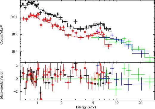
Top panel: XMM–Newton pn and MOS (black and red points, respectively) and NuSTAR FPMA and FPMB (green and blue points, respectively) spectral data and BF modelling (continuous lines); see the text for details. Bottom panel: spectral residuals in units of σ.
2.3 ALMA data
NGC 34 nuclear region was observed with ALMA in Band 9 during the Early Science Cycle 0 in 2012 May and August (project 2011.0.00182.S, PI: Xu), targeting the CO(6–5) transition (νrest-frame = 691.473 GHz) and the 435 μm dust continuum. The observing time is split in five execution blocks (EBs) with 16 antennas, set up in an extended configuration, and in one EB with 27 antennas, set up in both a compact and an extended configuration (the minimum baseline is 21 m, and the maximum baseline is 402 m). Hence, at the observing band, the largest angular scale (LAS) recovered by ALMA is ≈4 arcsec, corresponding to ∼2 kpc at NGC 34 distance, while the spatial resolution of the observation is θ ≃ 0.2 arcsec, corresponding to ∼100 pc. The field of view for the used 12 m antennas is FOV ≈9 arcsec. The medium precipitable water vapour of all the observing blocks is PWV ≃ 0.38 mm. The observation was performed in time division mode with a shallow velocity resolution of 6.8 km s−1, with four spectral windows of ≈2 GHz, centred at the sky frequencies of 679.8, 678.0, 676.3, and 674.3 GHz, respectively. The on-source integration time is about 2.25 h. The phase, bandpass, and flux calibrators observed are 2348-165, 3C 454.3, and the asteroid Pallas, respectively, and are the same for all the EBs. The analysis of the data obtained with a standard pipeline was reported by Xu et al. (2014).
Cycle 0 data reprocessing is strongly recommended, since, thanks to the new flux model libraries available (Butler-JPL-Horizons 2012), a more reliable flux calibration can be obtained (Butler 2012).3 Therefore, we took the raw data from the archive, we generated new reduction scripts, and we calibrated the data using casa 4.5.2, correcting for antenna positions, atmosphere effects, and electronics. Since these data are Band 9 observations, the calibrators are faint and the signal-to-noise ratio of the solutions is low, so that a phase solution over 60 s and a bandpass solution over 30 channels can be obtained. In addition, we put the signal-to-noise threshold equal to 1.5 (3 would be the recommended value) to find as many solutions as possible. Then, we applied the more reliable flux calibration, obtaining, for the calibrators, a ≈ 20 per cent higher flux density than the one reported in the archive.
We applied the self-calibration, making the image of the emission by selecting only the channels where the emission line was detected, we built a model, and we found phase solutions averaged on 600 s (i.e. approximately two scans). Then, we iterated again and we found phase and amplitude solutions, averaging 1200 s and combining scans. We produced the channel map of the CO(6–5) transition with an rms of ≈6.5 mJy beam−1, subtracting the continuum, binning into channels with a width of ≈34 km s−1, in order to increase the signal-to-noise ratio, and iteratively cleaning the dirty image, selecting a natural weighting scheme of the visibilities.
Fig. 2 shows the integrated emission of the CO(6–5) transition. Considering the emission within 3σ, contained in a diameter of θ ≈ 1.2 arcsec (≈500 pc), we obtain an integrated flux of (707 ± 106) Jy km s−1 (i.e. (1.63 ± 0.24) × 10−14 erg s−1 cm−2) with a peak of (213 ± 32) Jy km s−1. The rms of the image is ≈1.5 Jy beam−1 km s−1. The errors are totally dominated by the calibration error, which is the 15 per cent of the total flux in Band 9 for Cycle 0 Data. Our integrated flux is ≈ 30 per cent lower than the one reported by Xu et al. (2014). The cause of this discrepancy is likely due to the different flux calibration and the use of the new version of the casa software in our analysis.
![Integrated emission of the CO(6–5) line. The wedge on the right shows the colour scale of the map in Jy beam−1 km s−1. The integrated flux density is (707 ± 106) Jy km s−1. The contours at [3,10,20,50,100] are set in units of the rms noise level of the image, rms ≈1.5 Jy beam−1 km s−1.](https://oup.silverchair-cdn.com/oup/backfile/Content_public/Journal/mnras/474/3/10.1093_mnras_stx3011/1/m_stx3011fig2.jpeg?Expires=1749854133&Signature=nI-qFVr~aIKf9RhIAVwwlMwc6fjtZYDTzQcN27rlty39Rm3g8b~aKgbOH~SqO8GvnlPgLdGqMch6yHwHftZ~tQPLPci8djYlnpx37WcK3JMzdjtCPtZxIZGrCyHRLliwLmahGidTZB3abwg1XmPuGFhAwsfgtkTdzCsZ4vmuKlrh28lXJTjnkkPZI025EnUoJM-TtbctJDGDpLZuEk6BGttWoBTNxNNQgl-eA47Xyvd3zwKVJ-0RjCzBQu90HO8tyVNj-ZQdWwMQPOqP0ruRXaWAND3LsVGHMbWERru3650Rb8cKDrkjMQd5n7WMjShzOCWgIp976IdhFPlxkPXClA__&Key-Pair-Id=APKAIE5G5CRDK6RD3PGA)
Integrated emission of the CO(6–5) line. The wedge on the right shows the colour scale of the map in Jy beam−1 km s−1. The integrated flux density is (707 ± 106) Jy km s−1. The contours at [3,10,20,50,100] are set in units of the rms noise level of the image, rms ≈1.5 Jy beam−1 km s−1.
2.4 CO data
NGC 34 CO SLED is shown in Fig. 3, where the CO rotational transitions up to Jup = 13 are reported. The low-J transitions are ground-based observations. The CO(1–0) transition (blue square) was observed by CARMA, which covered an FOV ≈1.7 arcmin, detecting a regularly rotating disc of molecular gas with a diameter of 2.1 kpc (Fernández et al. 2014). The CO(2–1) transition (yellow triangle) was observed by the Submillimeter Array (SMA) with an FOV ≈22 arcsec (Ueda et al. 2014). By comparing the observed flux with the single-dish measurement made with the Swedish ESO Submillimeter Telescope, which covered an FOV ≈1 arcmin (Albrecht, Krügel & Chini 2007), we note that SMA recovered all the flux (Ueda et al. 2014). The observation of the CO(3–2) transition (purple pentagon) was conducted with the Submillimeter Telescope with an FOV ≈22 arcsec and the measure was corrected for subsequent comparison to Herschel CO lines (Kamenetzky et al. 2016). The CO(6–5) transition (red diamond) was observed by ALMA and recalibrated through the procedure outlined in Section 2.3, while the transitions from Jup = 4 to Jup = 13 (green circles) are Herschel/SPIRE observations, sparsely covering an FOV ≈2 arcmin (Rosenberg et al. 2015). NGC 34 appears point-like in the Herschel/SPIRE photometric bands (from 250 to 500 μm), characterized by a beam size of 17–42 arcsec (|${\approx }7\!{-}\!20\rm {\, } kpc$|). Assuming that the dust (sampled by the SPIRE photometric observations) and the gas (sampled by SPIRE/FTS observations) are almost cospatial, it can be argued that all the CO fluxes correspond to the integrated emission of the galaxy. By comparing the two different data sets for the CO(6–5) transition, we find a good agreement within 1σ. This allows us to be confident that the ALMA observation has recovered all the flux, which means that no flux related to the CO(6–5) emission comes from a region larger than the one observed with ALMA. Moreover, since ALMA LAS is comparable in size to the CO(1–0) disc (LAS ≈2 kpc, see Section 2.3), we can assume that no flux has been lost on the largest scales. Hence, all the data taken from the literature map the source entirely and are thus comparable in size.
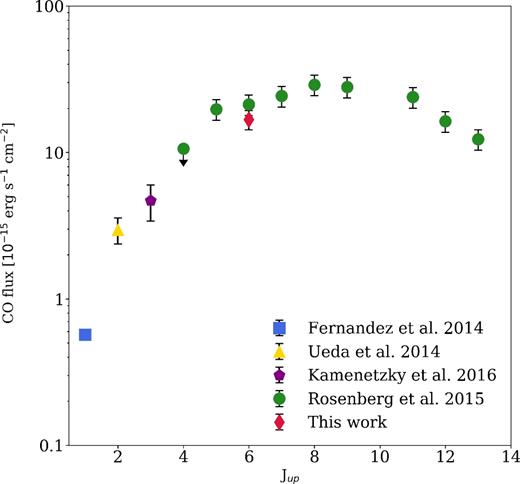
Observed CO flux of NGC 34 as a function of the upper J rotational level. The blue square, yellow triangle and purple pentagon represent the ground-based observations (Fernández et al. 2014; Ueda et al. 2014; Kamenetzky et al. 2016), the red diamond the CO(6–5) transition observed with ALMA and the green circles the Herschel/SPIRE FTS data from Jup = 4 to Jup = 13 (Rosenberg et al. 2015).
3 INTERPRETING THE CO SLED OF NGC 34
To fit and interpret the CO SLED of NGC 34, we have modelled the effect of the FUV and X-ray radiation on the molecular gas with the version c13.03 of cloudy (Ferland 2013), and the effect of the mechanical heating by adopting the shock models of Flower & Pineau des Forêts (2015). In what follows, we separately discuss their main features.
3.1 PDR and XDR modelling
We run a grid of cloudy PDR and XDR models that span ranges in density (n), distance between the source, and the illuminated slab of the cloud (d),4 and column density (NH). In these models, the external radiation field impinges the illuminated face of the cloud, which is assumed to be a 1D gas slab with a constant density, at a fixed distance from the central source (i.e. the collective light of stars in PDRs and an X-ray point-like source in XDRs).
For the PDR models, the SED of the stellar component is obtained using the stellar population synthesis code starburst99, assuming a Salpeter initial mass function in the range 1–100 M⊙, Lejeune–Schmutz stellar atmospheres (Schmutz, Leitherer & Gruenwald 1992; Lejeune, Cuisinier & Buser 1997), solar metallicity, and a continuous star formation mode, which is normalized to NGC 34 SFR (≃ 24 M⊙ yr−1; Gruppioni et al. 2016). We assume a Milky Way gas-to-dust ratio of ≈160 (e.g. Zubko, Dwek & Arendt 2004) for the gas slab. We run 21 PDR models, varying n in the range log(n/cm−3) = [2–4.5] and the distance of the gas slab from the radiation source in the range d = [100–500] pc. These values of distances translate into a flux in the FUV band normalized to that observed in the solar neighbourhood (1.6 × 10 − 3 erg s − 1 cm − 2; Habing 1968), in the range [104–103] G0, respectively. The code computes the radiative transfer through the slab spanning a hydrogen column density range log(NH/cm−2) = [19–23]. The densities and column densities are chosen to cover the typical values in giant MCs (McKee & Ostriker 1977). We constrain the range of distances to be larger than the ALMA minimum recoverable scale (≈100 pc, see Section 2.3).
In the XDR models, the AGN radiation field is modelled following the default table AGNcloudy command (Korista, Ferland & Baldwin 1997), and its spectrum is normalized so that the 1–100 keV X-ray luminosity matches the observed one |$L_{\mathrm{1\!{-}\!100{\, }keV}}\simeq 4 \times 10^{42}$| erg s−1 (see Section 2.2). We run nine models, adopting a slightly higher range of densities log(n/cm−3) = [3.5–5.5] and the same values of column densities and distances, which translate into an X-ray flux at the cloud surface FX ≃ 2.2–0.2 erg cm−2 s−1.
3.2 Shock modelling
The Flower & Pineau des Forêts (2015) shock code simulates shocks in the ISM as a function of the physical conditions in the ambient gas, providing the CO line intensities (i.e. fluxes per unit of the emitting area where the shock acts, A). Shock waves in the ISM can be distinguished in ‘jump’ (J) or ‘continuous’ (C) types, according to the strength of the magnetic field and the ionization degree of the medium in which they propagate (see e.g. fig. 1 in Draine 1980). In J-shocks, the variation in the fluid properties (density, temperature, and velocity) occurs sharply and can be approximated as a discontinuity. In C-shock models, instead, the influence of the magnetic field on the ionized gas causes the ions to diffuse upstream of the shock front, thus eliminating the discontinuities in the fluid variables (Draine & McKee 1993; Pon, Johnstone & Kaufman 2012). These differences cause the J-shock temperature (T≈104 K) to be far higher than the one characterizing C-shock (T≈103 K), inducing the dissociation of H2 molecules (Flower & Pineau Des Forêts 2010). This is the reason why C-type shocks are preferentially invoked to affect the CO emission in MCs (e.g. Smith & Mac Low 1997; Hailey-Dunsheath et al. 2012).
In this work, we compare the observed CO SLED with two grids of C- and J-shock models, respectively. We let the shock velocity5 vary in the range |$v_{\rm sh}=[10\!{-}\!40] \rm {\, } {\, } km{\, } s^{-1}$|, and the pre-shock density in log(n/cm−3) = [3–6]. The transverse magnetic field scales with the density through the relation B ∼ bn1/2, where b = 1 for C-shocks, and b = 0.1 for J-shocks (Flower & Pineau des Forêts 2015).
3.3 CO SLED fitting
Despite the good spatial resolution of ALMA (see Section 2.3), individual clouds in extragalactic sources cannot be resolved. Each resolution element in ALMA observations measures the combined emission from a large ensemble of MCs. Moreover, as pointed out in Section 1, low-J CO transitions are generally excited in the cold diffuse component of molecular gas while mid- and high-J transitions are associated with a warmer and denser component. The observed CO SLED of NGC 34 can then be reproduced by summing a low-density PDR component (e.g. log(n/cm−3) ≃ 2–2.5) that accounts for the low-J transitions, to a second component for the high-J transitions. Given the spatial constraints on the CO(1–0) emission (see Section 2.4), the low-density PDR must account for the emission of MCs located within d < 1 kpc from the centre of the galaxy. In addition, we fixed the gas column density of the low-density PDR to log(NH/cm−2) ≃ 21.8, which is slightly above that (log(NH/cm−2) ≃ 21.6) required to have CO molecules (van Dishoeck & Black 1988). The CO(6–5) emission line allows to constrain the high-density component in a region of d < 250 pc from the centre. We have adopted three different approaches to model this second component, which can be produced by either
a high-density PDR (PDR1+PDR2 model);
the shock heated gas (PDR+shock model); or
an XDR (PDR+XDR model).
The PDR1+PDR2 and the PDR+shock models are shown in Fig. 4, in the upper and lower panels, respectively. The black solid line represents the sum of the components, while the 1σ confidence levels on the normalizations have been obtained by marginalizing over the other parameters and considering a Δχ2 = 2.3 (Lampton, Margon & Bowyer 1976). The PDR+XDR model is shown in Fig. 5. All the parameters taken into account and their BF values are summarized in Table 1.
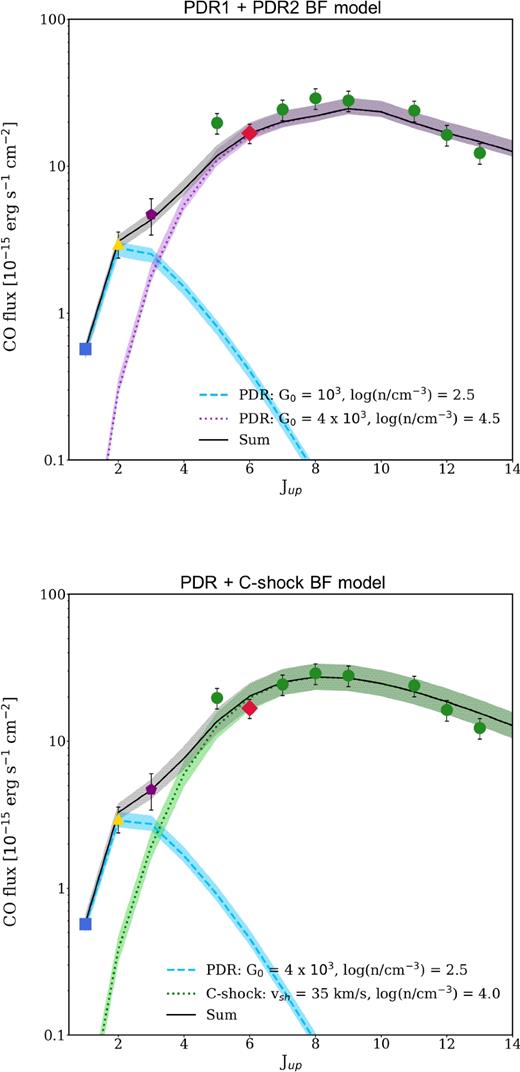
Top panel: PDR1+PDR2 BF model, overplotted to the observed data. The light-blue dashed line and the purple dotted line represent the low-density and high-density PDRs, respectively. Bottom panel: PDR+C-shock BF model, overplotted to the observed data. The light-blue dashed line and the green dotted line indicate the low-density PDR and the C-shock component, respectively. In these figures, the black solid line indicates the sum of the two components and the shaded areas indicate the ±1σ uncertainty range on the normalization of each component.

Fiducial model (PDR+XDR), overplotted to the observed data. The light-blue dashed line and the red dotted line represent the low-density PDR and the high-density XDR, respectively. The black solid line indicates the sum of the two components and the shaded areas indicate the ±1σ uncertainty range on the normalization of each component.
PDR1+PDR2 and PDR+C-shock BF models, and PDR+XDR fiducial model parameters. For PDRs and XDRs, the distance from the source, the density, and the column density values are reported. Density and column density values are given in logarithm. For C-shocks, the shock velocity, the pre-shock density, and the shock-related emitting area are reported. The * means that the value was fixed in the chi-square analysis. Finally, the χ2 and degrees of freedom (dof) values are indicated.
| d | n | N | |
|---|---|---|---|
| Best fit | (pc) | (cm−3) | (cm−2) |
| PDR1 | 500 | 2.5 | 21.8* |
| PDR2 | 250 | 4.5 | 21.7 |
| χ2/dof | 13.2/4 | ||
| Best fit | d | n | N |
| (pc) | (cm−3) | (cm−2) | |
| PDR | 500 | 2.5 | 21.8* |
| vsh | n | A | |
| (km s−1) | (cm−3) | (pc2) | |
| C-shock | 35 | 4.0 | (785)2 |
| χ2/dof | 9.9/5 | ||
| Best fit | d | n | N |
| (pc) | (cm−3) | (cm−2) | |
| PDR | 500 | 2.5 | 21.8* |
| XDR | 100 | 4.5 | 23.0* |
| χ2/dof | 7.8/5 |
The PDR1+PDR2 BF model is characterized by a value of the reduced-χ2 (|$\tilde{\chi }^2$|), defined as the ratio between the computed χ2 and the related degrees of freedom, of |$\tilde{\chi }^2_{\rm BF}= 3.3$|. Such a high value made us infer that the high-density PDR cannot reproduce completely the high-J transitions.
The PDR+C-shock BF model has instead a slightly lower |$\tilde{\chi }^2_{\rm BF}$| (=2.0). However, the best fit for the C-shock-heated component, accounting for the high-J CO emission, returns an emitting area (A = 7852 pc2) that is 10× larger than the CO(6–5) emitting region.6
The PDR+XDR BF has the lowest |$\tilde{\chi }^2_{\rm BF}$| among all the combinations tested in this work (|$\tilde{\chi }^2_{\rm BF} = 1.6$|); therefore, it is our fiducial model. It is composed by a ‘cold’ and diffuse PDR (T ≃ 30 K, log(n/cm−3) ≃ 2.5), which accounts for the CO(1–0) and the CO(2–1) transitions, produced by clouds located at a typical distance d ≃ 500 pc from the source of the FUV radiation (i.e. OB stars), and by a ‘warm’ and dense XDR (T ≃ 65 K, log(n/cm−3) ≃ 4.5), composed by clouds located at d ≃ 100 pc from the central X-ray source. In this case, we fixed the XDR column density to a typical value of log(NH/cm−2) ≃ 23.0, since X-rays can penetrate deeper into the molecular gas (e.g. Meijerink & Spaans 2005). The radiation penetrates up to a depth l ≈ 5.0 pc for the PDR, and up to l ≈ 0.3 pc, for the XDR. These values are in line with the typical environment sizes of giant MCs, clumps, and cores, respectively, as reported by McKee & Ostriker (2007). From our fiducial modelling, we estimate a total mass Mgas ≃ 3.1 × 10⁹ M⊙ (typical value of LIRGs; e.g. Papadopoulos 2010), which appears to be completely dominated by the low-density component that accounts for |$M= (2.9^{+0.9}_{-0.8}) \times 10^9$| M⊙, whereas the warm component contribution is |$M= (2.3^{+0.4}_{-0.5}) \times 10^8$| M⊙. This value is consistent with the total molecular mass found by Fernández et al. (2014), who estimated Mgas = (2.1 ± 0.2) × 109 M⊙, considering the CO(1–0) luminosity and the standard conversion factor for starburst systems αCO ≃ 0.8 M⊙/(K km s−1 pc2) (Solomon et al. 1997). From our estimate of the total mass, we infer that in NGC 34 αCO ≃ 1.1 M⊙/(K km s−1 pc2). This value is consistent with that reported by Bolatto, Wolfire & Leroy (2013) concerning LIRGs.
To complete our analysis, we also explored the possibility of a three-component model accounting for the PDR, XDR, and shock heating contribution. We fixed the column densities of the PDR and the XDR to log(NH/cm−2) = 21.8 and log(NH/cm−2) = 23.0, respectively, and the shock-related emitting area to the CO(6–5) emission size (∼2502 pc2). The BF model has a |$\tilde{\chi }^2_{\rm BF}= 2.4$| and is shown in Fig. 6, while its parameters are reported in Table 2. We compare this new configuration with our fiducial PDR+XDR model, taking advantage of the Fisher test, as presented by Bevington & Robinson (2003). We find a value of f = 0.66 that corresponds to a probability P(F ≤ f) = 70 per cent, which means that the addition of a third component brings a negligible improvement in the CO SLED fit. This does not mean that shocks are completely absent within the galaxy, but that they do not play a significant role in exciting the high-J CO transitions, more likely powered by the central AGN.
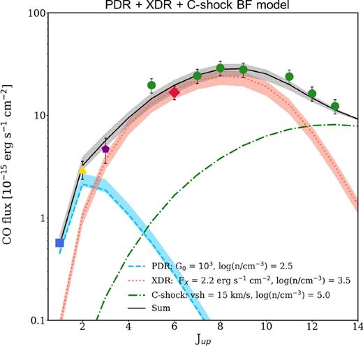
PDR+XDR+C-shock BF model overplotted to the observed data. The light-blue dashed line and the red dotted one indicate the low-density PDR and the XDR, respectively, whereas the green dot–dashed line represents the C-shock. The solid black line indicates the sum of the three components and the shaded areas indicate the ±1σ uncertainty range on the normalization of each component.
BF model (PDR+XDR+C-shock) parameters. For PDRs and XDRs, the values reported are the distance from the source, the density, and the column density, respectively. Density and column density values are given in logarithm. For C-shocks, the shock velocity, the pre-shock density, and the shock-related emitting area are reported. The * means that the value was fixed in the chi-square analysis. Finally, the χ2 and degrees of freedom (dof) value are indicated.
| d | n | N | |
|---|---|---|---|
| Best fit | (pc) | (cm−3) | (cm−2) |
| PDR | 500 | 2.5 | 21.8* |
| XDR | 100 | 3.5 | 23.0* |
| vsh | n | A | |
| (km s−1) | (cm−3) | (pc2) | |
| C-SHOCK | 15 | 5.0 | (250)2* |
| χ2/dof | 7.1/3 |
| d | n | N | |
|---|---|---|---|
| Best fit | (pc) | (cm−3) | (cm−2) |
| PDR | 500 | 2.5 | 21.8* |
| XDR | 100 | 3.5 | 23.0* |
| vsh | n | A | |
| (km s−1) | (cm−3) | (pc2) | |
| C-SHOCK | 15 | 5.0 | (250)2* |
| χ2/dof | 7.1/3 |
3.4 Discussion and comparison with previous works
The CO SLED of NGC 34 has been extensively studied by others authors (e.g. Pereira-Santaella et al. 2014; Rosenberg et al. 2015).
Rosenberg et al. (2015) analysed a sample of LIRGs, including NGC 34, suggesting a qualitative separation on the basis of the shape of the CO ladder, the CO(1–0) linewidth, and the AGN contribution, trying to indicate which mechanisms are responsible for gas heating. They identify NGC 34 as a galaxy with a very flat CO ladder beyond the CO(7–6) transition, which indicates a significant emission by warm and dense molecular gas, that is due to another heating mechanism besides UV heating. This galaxy appears to have an inclination corrected CO(1–0) linewidth of ≃ 600 km s−1 and a low AGN contribution of the bolometric luminosity (≃ 30 per cent), and thus they infer that the molecular gas in NGC 34 is experiencing shock excitation.
Pereira-Santaella et al. (2014) have presented a CO emission modelling for NGC 34, using the non-equilibrium radiative transfer code radex (van der Tak et al. 2007), along with cloudy c13.02 PDR and shock models. They infer that a combination of both PDR and shock models is needed to reproduce the observed CO SLED in NGC 34. They also contend that, although X-ray heating can play a role in AGN, its contribution in LIRGs with high SFR and IR luminosity is negligible in the integrated spectra of the galaxy.
Our work, on the contrary, suggests that X-rays are important in the CO excitation in NGC 34, even though we do not completely exclude the contribution of shock heating. In Section 3.3, we show that, in order to reproduce the high-J CO emission only with shock models, we need a shock-emitting area far greater than the size of the CO(6–5) area observed with ALMA. This points towards a scenario in which X-ray heating of high-density gas is favourite against shocks to be the primary source of excitation of high-J CO lines. Even though it can be rather difficult to distinguish among shock and XDR heating, Meijerink et al. (2013) and Gallerani et al. (2014) suggest that the CO-to-IR continuum ratio (LCO/LIR) can be a key diagnostic for the presence of shocks. Shocks only heat the gas without affecting the temperature of dust grains, which are the primary source of the IR emission (Hollenbach et al. 1989; Meijerink et al. 2013) and thus produce high values (LCO/LIR > 10−4) for the CO-to-IR continuum ratio. NGC 34 has an observed CO-to-IR continuum ratio of LCO/LIR ≃ 2.7 × 10⁻⁵, which is almost a factor 4 lower than the threshold. This supports our conclusion that even though shocks are expected to be frequent in the highly supersonic turbulent molecular gas found in LIRGs, they are probably not dominant in the powering of high-J transitions in the observed CO SLED of NGC 34. In this scenario, the large linewidth of the CO(1–0) would not be indicative of shocks, but probably traces the rotation of the 2.1 kpc disc resolved by Fernández et al. (2014). We stress that our result is not in contradiction with the relatively low fraction (LX/Lbol ∼ 10 per cent) of NGC 34, as in our XDR modelling we have properly scaled our AGN radiation to reproduce the X-ray luminosity of the galaxy.
In the local Universe, a modelling that requires an XDR component to explain the high-J transitions has been proposed also by van der Werf et al. (2010) for the nearby ULIRG Mrk 231, and by Pozzi et al. (2017) for NGC 7130, a nearby ‘ambiguous’ LIRG, similar to NGC 34. Both Mrk 231 and NGC 7130 are obscured objects with an intrinsic X-ray luminosity of ∼1043 erg s−1, and thus NGC 34, characterized by |$L_{\rm {2\!{-}\!10{\, }keV}} \sim 10^{42}$| erg s−1, would extend the importance of an XDR component to galaxies with a lower X-ray luminosity.
4 CONCLUSION
In this paper, we analysed archival XMM–Newton, NuSTAR, ALMA, and Herschel data and investigated the molecular CO emission as a function of the rotational level (CO SLED), in order to probe the physical properties of the gas, such as density, temperature, and the main source that causes the emission (star formation, AGN or shocks) in the Seyfert 2 and LIRG galaxy NGC 34, comparing PDR, XDR and shock models with the observations. The main steps of our work and our main conclusions can be summarized as follows.
The same model has been assumed simultaneously for XMM–Newton and NuSTAR data over a broad energy range, fixing the power-law photon indices to Γ = 1.9. We find an obscuration of |$N_{\rm {H}}=5.2^{+1.3}_{-1.1}\times 10^{23}$| cm−2, an observed 2–10 keV flux of 3.2× 10⁻¹³ erg cm−2 s−1, and an intrinsic (i.e. corrected for the obscuration) rest-frame 2–10 keV and 1–100 keV luminosities of 1.3 × 1042 erg s−1 and 4.0 × 1042 erg s−1, respectively. The 1–100 keV luminosity is used to run Cloudy XDR models.
ALMA Cycle 0 data of the CO(6–5) line emission have been analysed starting from the raw data available in the archive. The CO(6–5) integrated flux results to be (707 ± 106) Jy km s−1 with a peak of (213 ± 32) Jy km s−1. The emission comes from a region with a diameter of θ ≈ 1.2 arcsec, which corresponds to a physical scale of ≈500 pc.
We infer that a PDR1+PDR2 or a PDR+shock model is unlikely to reproduce the observed CO SLED. The former is discarded because of the high value of the |$\tilde{\chi }^2$|, while the latter has a BF value of the shock-emitting area that appears to be at least 10× higher than the region associated with the CO(6–5) emission, while shocks are expected to account for the high-J transitions.
The observed CO SLED of NGC 34 can be explained by a cold and diffuse PDR (T ≃ 30 K, log(n/cm−3) ≃ 2.5, G0 = 103), which accounts for the low-J transitions and a warmer and denser XDR (T ≃ 65 K, log(n/cm−3) ≃ 4.5, FX ≃ 2.2 erg cm−2 s−1), necessary to explain the high-J transitions. The existence of a warm XDR component is supported by the χ2-square analysis and by all the pieces of evidence of a possible AGN in the central region of NGC 34 discussed in Section 2.1. We conclude that the AGN contribution is significant in heating the molecular gas in NGC 34.
The estimated molecular gas mass is Mgas ≃ 3.1 × 10⁹ M⊙. We note that the diffuse component contribution to the total mass is dominant compared to the warmer component (one order of magnitude lower). From our total mass estimate, we infer an αCO of 1.1 M⊙/(K km s−1 pc2) for NGC 34.
According to the F-test analysis, a three-component model composed by a PDR, an XDR, and a C-shock is not significantly improved with respect to our fiducial model (PDR+XDR).
Our results shed light on the great potential of combining self-consistent multiband and multiresolution data in order to assess the importance of an AGN and star formation activity, and mechanical heating produced by shocks for the physics of molecular gas. Papadopoulos et al. (2012) and Imanishi, Nakanishi & Izumi (2016) proposed that, in addition to CO rotational lines, a combination of low- to mid-J rotational lines of heavy rotor molecules with high critical densities, such as HCO+, HCN, HNC, and CN, can be used to probe the large range of physical properties within MCs (Tkin ∼ 15–100 K, n(H2) ∼ 102–106 cm−3; e.g. McKee & Ostriker 2007). For instance, HCO+ line appears to be stronger in XDRs than in PDRs by a factor of at least 3, while CN/HCN ratio is far higher in PDRs than in XDRs, where it is expected to be ∼5–10 (Meijerink, Spaans & Israel 2007). Therefore, high-resolution observations of high critical density molecules with ALMA, characterized by a very high spatial and spectral resolution, could provide new insights on physical properties of NGC 34 and similar nearby composite objects.
Acknowledgements
We thank the Italian node of the ALMA Regional Center (ARC) for the support. This paper makes use of the following ALMA data: ADS/JAO.ALMA#2011.0.00182.S. ALMA is a partnership of ESO (representing its member states), NSF (USA), and NINS (Japan), together with NRC (Canada) and NSC and ASIAA (Taiwan), in cooperation with the Republic of Chile. The Joint ALMA Observatory is operated by ESO, AUI/NRAO, and NAOJ. We kindly thank also G. Zamorani for his useful advice and the anonymous referee for her/his comments and suggestions, which significantly contributed to improving the quality of the publication.
Footenotes
In the solar neighbourhood, the typical scale of MCs is ≈ 45 pc (Blitz 1993).
A 1 keV photon penetrates up to a typical column of NH ≃ 2 × 1022 cm−2, whereas a 10 keV photon penetrates NH ≃ 4 × 1025 cm−2 (Schleicher, Spaans & Klessen 2010).
Butler (2012) contends that many of the models used to calculate the flux density of Solar system bodies in the 2010 version were inaccurate with respect to the new ones of 2012, which use new brightness temperature models, and a new flux calculation code that replaces the ‘Butler-JPL-Horizons 2010’ standard used before.
A larger distance from the source implies a lower incident radiation field, since the flux is proportional to d−2. Hence, taking into account different values of distance means to vary the incident radiation field.
Shock velocities greater than 50 km s−1 are known to be fast enough to destroy molecules (Hollenbach et al. 1989).
Note that in case of a J-shock, the emitting area A required to fit the data would be 1000× larger than the CO(6–5) emitting region. That is why, we decided not to show the PDR+J-shock BF model.
