


Abstract
In this paper, we study an anisotropic universe model with Bianchi-I metric using Joint light-curve analysis (JLA) sample of Type Ia supernovae (SNe Ia). Because light-curve parameters of SNe Ia vary with different cosmological models and SNe Ia samples, we fit the SNe Ia light-curve parameters and cosmological parameters simultaneously employing Markov chain Monte Carlo method. Therefore, the results on the amount of deviation from isotropy of the dark energy equation of state (δ), and the level of anisotropy of the large-scale geometry (Σ0) at present, are totally model-independent. The constraints on the skewness and cosmic shear are −0.101 < δ < 0.071 and −0.007 < Σ0 < 0.008. This result is consistent with a standard isotropic universe (δ = Σ0 = 0). However, a moderate level of anisotropy in the geometry of the Universe and the equation of state of dark energy, is allowed. Besides, there is no obvious evidence for a preferred direction of anisotropic axis in this model.
1 INTRODUCTION
Astronomical observations revealed that our Universe is undergoing an accelerating expansion (Riess et al. 1998;Perlmutter et al. 1999), which is one of the most surprising astronomical discoveries in recent years. Accelerating expansion implies that the universe is dominated by an unknown form of energy called ‘dark energy’ with negative pressure, or that Einstein’s theory of gravity fails on cosmological scales and requires some modifications.
The standard Lambda cold dark matter (ΛCDM) model is established based on the cosmological principle and parametrization of the big bang cosmological model. It depicts a homogeneous and isotropic universe on large scales with approximately 30 per cent matter (including baryonic matter and dark matter) and 70 per cent dark energy at present time, which is consistent with vast majority of several precise astronomical observations, including cosmic microwave background (CMB) power spectrum (WMAP Collaboration 2011; Planck Collaboration XIII 2016) and baryon acoustic oscillations (Eisenstein et al. 2005).
However, the standard cosmological model is challenged by a few puzzling cosmological observations (Perivolaropoulos 2014), which may require modifications. Evidence for cosmology anisotropy has been obtained by the power asymmetry of CMB perturbation maps (Eriksen et al. 2007; Hoftuft et al. 2009; Paci et al. 2010; Mariano & Perivolaropoulos 2013; Zhao & Santos 2015), the large-scale velocity flows (Kashlinsky et al. 2008; Watkins, Feldman & Hudson 2009; Feldman, Watkins & Hudson 2010; Kashkinsky et al. 2010; Lavaux et al. 2010), anisotropy in accelerating expansion rate (Antoniou & Perivolaropoulos 2010; Mariano & Perivolaropoulos 2012; Wang & Wang 2014; Yang, Wang & Chu 2014), spatial dependence of the value of the fine structure constant α (Moss et al. 2011; Webb et al. 2011; King et al. 2012; Mariano & Perivolaropoulos 2012; Pinho et al. 2016) and so on. These puzzles are in favour of preferred cosmological directions, which seem to violate the cosmological principle. The so-called ‘cosmic anomalies’ (Perivolaropoulos 2014) may either be simply large statistical fluctuations or have some physical origins, which could be either geometric or energy-related (Perivolaropoulos 2014).
Here, we focus on an anisotropic universe model that has a plane-symmetric Bianchi – I metric (Taub 1951; Aluri et al. 2013; Schücker, Tilquin & Valent 2014), namely ellipsoidal universe (Campanelli, Cea & Tedesco 2006). The ellipsoidal universe model was first proposed in Campanelli et al. (2006) to solve the CMB quadrupole problem by assuming a plane-symmetric universe with an eccentricity of the order of 10−2 at decoupling. Campanelli, Cea & Tedesco (2007) discussed that the anisotropic expansion can be generated by cosmological magnetic fields, cosmic domain walls or cosmic strings. The cosmic shear Σ0 and skewness δ are introduced (Campanelli et al. 2011a) to describe the anisotropy level of cosmic geometry and dark energy fluids, respectively. Campanelli et al. (2011c) analysed Union and Union2 compilation and concluded that an isotropic universe is consistent with Type Ia supernovae (SNe Ia) data. However, their analysis directly used μobs and σ obtained in ΛCDM model (Amanullah 2010). The results are model-dependent, because light-curve parameters change with different universe models and SNe Ia sample. Schücker et al. (2014) fitted the Bianchi – I metric to the Hubble diagram of SNe Ia.
Therefore, we improve the previous research by fitting the SNe Ia light-curve parameters and cosmological parameters simultaneously. This paper is organized as follows. In the next section, we introduce the ellipsoidal universe model and derive the magnitude–redshift relation. In Section 3, we use SNe Ia data of Joint light-curve analysis (JLA) sample to constrain all the free parameters simultaneously, including light-curve and cosmological parameters. The fitting results are shown in Section 4. Conclusion and discussions are given in Section 5.
2 ELLIPSOIDAL UNIVERSE MODEL
2.1 Anisotropy axis
2.2 Redshift–distance relation
3 JLA SAMPLE AND MCMC FITTING
The JLA sample (Betoule et al. 2014) is based on Conley et al. (2011) compilation. It includes three-season data from SDSS-II (0.05 < z < 0.4), three-year data from SNLS (0.2 < z < 1), HST data (0.8 < z < 1.4), and several low-redshift samples (z < 0.1) such as Calán/Tololo Survey and Carnegie Supernova Project. The JLA sample totals 740 spectroscopically confirmed SNe Ia with high-quality light curves.
3.1 Angular position
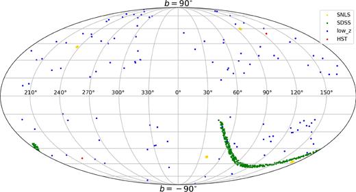
Angular positions of SNe Ia in the JLA sample. b (−90° ≤ b ≤ 90°) is the galactic latitude and l (0° ≤ l < 360°) is the galactic longitude. SNe from four subsets are marked with different colours.
3.2 Distance modulus
3.3 The hubble diagram covariance matrix
Cstat is obtained from error propagation of light-curve fit uncertainties. The systematic uncertainties include seven components, namely the calibration uncertainty |${\bf C}$|cal, the light-curve model uncertainty |${\bf C}$|model, the bias correction uncertainty |${\bf C}$|bias, the mass step uncertainty |${\bf C}$|host, the peculiar velocity uncertainty |${\bf C}$|pecvel, and the non-Ia events uncertainty |${\bf C}$|nonIa.
Values of σcoh used in the cosmological fits for different samples.
| Sample | Low-z | SDSS-II | SNLS | HST |
|---|---|---|---|---|
| |$\boldsymbol{\sigma _{{\rm coh}}}$| | 0.134 | 0.108 | 0.080 | 0.100 |
| Sample | Low-z | SDSS-II | SNLS | HST |
|---|---|---|---|---|
| |$\boldsymbol{\sigma _{{\rm coh}}}$| | 0.134 | 0.108 | 0.080 | 0.100 |
3.4 Markov chain Monte Carlo fitting
The priors of free parameters in MCMC fitting.
| Parameter | Prior | Parameter | Prior |
|---|---|---|---|
| α | [0.1, 0.2] | Σ0 | [−0.5, 0.5] |
| β | [2.0, 4.0] | w | [−2.0, 0.0] |
| |$M_B^1$| | [−19.3, -18.6] | δ | [−0.5, 0.5] |
| ΔM | [−0.1, 0.0] | lA | [0, π] |
| H0 | [60, 80] | bA | [|$-\frac{\pi }{2}$|, |$\frac{\pi }{2}$|] |
| Ωm | [0.0, 0.5] |
Campanelli et al. (2011c) studied an anisotropic Bianchi type I cosmological model using Union2 compilation, in which μobs and σ are derived in the ΛCDM model (Amanullah 2010). Therefore, the light-curve parameters {|$\alpha , \beta , M_B^1, \Delta _M$|} are fixed. However, the light-curve parameters vary with different cosmological model. It’s unreasonable to fit just cosmological parameters. Different from Campanelli et al. (2011c), we fit four light-curve parameters and seven cosmological parameters {H0, Ωm, Σ0, w, δ, lA, bA} simultaneously. So the likelihood function depends on eleven free parameters. The derived results are model-independent.
As a comparison, we carried out another MCMC fitting, which constrained parameters {|$\alpha , \beta , M_B^1, \Delta _M, H_0, \Omega _{\rm m}, w$|} in a flat wCDM cosmology with an arbitrary equation of state w.
4 RESULTS
The confidence contours (1σ, 2σ and 3σ) and marginalized likelihood distribution functions for the parameters (|$\alpha , \beta , M_B^1, \Delta _M, H_0, \Omega _{\rm m}, \Sigma _0, w, \delta$|) from MCMC fittings are shown in Fig. 2. Table 3 lists the best-fitting value and the 1σ, 2σ, and 3σ confidence level intervals. Since |$M_B^1$| entirely degenerates with H0, their values cannot be constrained well simultaneously. If we take Hubble constant H0 = 73.24km s−1 Mpc−1 (Riess et al. 2016), the corresponding |$M_B^1$| is −18.95.
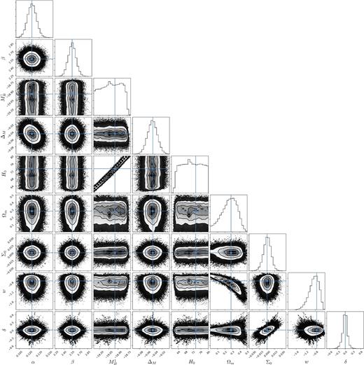
Confidence contours (1σ, 2σ and 3σ) and marginalized likelihood distributions for the parameters (|$\alpha , \beta , M_B^1, \Delta _M, H_0, \Omega _{\rm m}, \Sigma _0, w, \delta$|) in ellipsoidal universe model. True values (shown as dots) of {|$\alpha , \beta , M_B^1, \Delta _M, \Omega _{\rm m}, w$|} are taken from wCDM fitting results as comparison.
Best-fitting values, and the 1σ, 2σ, and 3σ confidence level intervals derived from the JLA sample.
| α | β | ΔM | Ωm | Σ0 | w | δ | |
|---|---|---|---|---|---|---|---|
| BF | 0.124 | 2.554 | −0.045 | 0.314 | 0.001 | −0.774 | −0.008 |
| 1σ | [0.118, 0.131] | [2.475, 2.622] | [−0.059, −0.032] | [0.173, 0.383] | [−0.007, 0.008] | [−1.028, −0.633] | [−0.101, 0.071] |
| 2σ | [0.111, 0.137] | [2.406, 2.701] | [−0.072, −0.020] | [0.046, 0.443] | [−0.015, 0.015] | [−1.296, −0.535] | [−0.236, 0.185] |
| 3σ | [0.105, 0.144] | [2.335, 2.777] | [−0.086, −0.007] | [0.003, 0.488] | [−0.024, 0.023] | [−1.527, −0.468] | [−0.451, 0.388] |
Comparisons between best-fitting values in wCDM model and ellipsoidal universe model.
| α | β | |$M_{B}^1$| | ΔM | Ωm | w | |
|---|---|---|---|---|---|---|
| wCDM | 0.124 | 2.554 | −18.95 | −0.045 | 0.281 | −0.750 |
| Ellipsoidal | 0.124 | 2.554 | −18.95 | −0.045 | 0.314 | −0.774 |
| α | β | |$M_{B}^1$| | ΔM | Ωm | w | |
|---|---|---|---|---|---|---|
| wCDM | 0.124 | 2.554 | −18.95 | −0.045 | 0.281 | −0.750 |
| Ellipsoidal | 0.124 | 2.554 | −18.95 | −0.045 | 0.314 | −0.774 |
The best-fitting results of the flat wCDM model are displayed in Fig. 4 for comparison. We find that best-fitting values of parameters in ellipsoidal model are quite similar to those in the wCDM model (see Table 4). Considering that the best-fitting values of Σ0 and δ are nearly zero, and wCDM is the limiting case of ellipsoidal universe model, this result can be expected. Fig. 5 shows the Hubble diagram for JLA sample in two different cosmological models. One is the best-fitting model with (Ωm, Σ0, w, δ) = (0.314, 0.001, −0.774, −0.008) (blue dashed line). The other is the flat wCDM model with Ωm = 0.281, w = −0.750 (black line). In the lower panel, we show the corresponding distance modulus fitting residuals (distance modulus minus the best-fitting wCDM distance modulus) as a function of redshift. The comparison between the best-fitting values of cosmological parameters from Union2 (Campanelli et al. 2011c) and JLA sample is shown in Table 5. The constraints are more tight than those of Campanelli et al. (2011c).
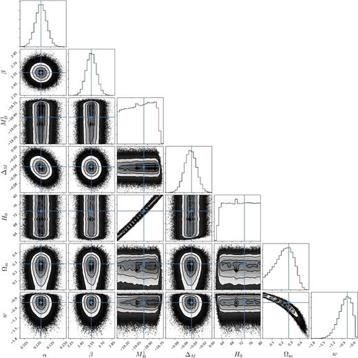
Confidence contours (1σ, 2σ and 3σ) and marginalized likelihood distribution functions for the parameters (|$\alpha , \beta , M_B^1, \Delta _M$|, H0, Ωm, w) in the wCDM model.
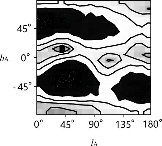
Confidence level contours of preferred direction in the galactic coordinate system.
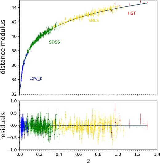
Upper panel: Hubble diagram for the 740 SNe Ia in the JLA compilation for different cosmological models: best-fitting ellipsoidal model (Ωm, Σ0, w, δ) ≃ (0.314, 0.001, −0.774, −0.008) (blue dashed line), and wCDM model (Ωm, w) ≃ (0.281, −0.750) (black line). Lower panel: residuals (distance modulus minus distance modulus for the wCDM model) for the same models in the upper panel.
Comparisons between best-fitting values of cosmological parameters from Union2 and JLA sample for ellipsoidal universe model.
| Σ0 | δ | Ωm | w | |
|---|---|---|---|---|
| Union2 | −0.004 | −0.050 | 0.37 | −1.32 |
| JLA | 0.001 | −0.008 | 0.314 | −0.774 |
| Σ0 | δ | Ωm | w | |
|---|---|---|---|---|
| Union2 | −0.004 | −0.050 | 0.37 | −1.32 |
| JLA | 0.001 | −0.008 | 0.314 | −0.774 |
5 CONCLUSIONS
Acknowledgements
We thank the anonymous referee for constructive comments. This work is supported by the National Basic Research Program of China (973 Program, grant No. 2014CB845800) and the National Natural Science Foundation of China (grants 11422325 and 11373022), and the Excellent Youth Foundation of Jiangsu Province (BK20140016).
REFERENCES
