The dynamical systems approach to numerical integration

Wisdom, Jack

doi:10.1093/mnras/stx2906

Abstract

The dynamical systems approach to numerical integration is reviewed and extended. The new method is compared to some alternative methods based on the Lie series approach. The test problem is the motion of the outer planets. The algorithms developed using the dynamical systems approach perform well.

gravitation, methods: numerical, planets and satellites: dynamical evolution and stability

1 INTRODUCTION

The integration method introduced by Wisdom & Holman (1991) and variations developed from it are used in most long-term studies of the evolution of planetary systems. The method is based on results from the theory of Hamiltonian dynamical systems (Chirikov 1979). The essential innovation of the method was to approximate the evolution of the n-body problem by interleaving the evolution of the Kepler problem with the evolution governed by the interactions. Wisdom & Holman (1991) used the Jacobi coordinates to effect the elimination of the centre of mass and split the Hamiltonian into Kepler and interaction terms. Subsequent variations have made use of different coordinate systems, or slightly different splittings of the n-body Hamiltonian, but the basic idea is the same.

The Wisdom & Holman (1991) method was used in the 100 Myr integration of Sussman & Wisdom (1992) of the full Solar system that demonstrated that the evolution of the Solar system is chaotic. This result confirmed the earlier result of Laskar (1989) that the evolution of the Solar system is chaotic. Note that the result of Laskar (1989) was uncertain because Laskar used an averaged and truncated model of the motion of the planets. It is well known that truncating an integrable problem can lead to chaotic behaviour. For instance, the integrable Toda problem, when truncated to degree three in the rectangular coordinates, can be transformed into the classic Hénon–Heiles problem (Contopoulos & Polymilis 1987). So a full integration was required to settle the issue of the chaotic character of the motion of the planets.

Wisdom, Holman & Touma (1996) introduced several extensions of the original method of Wisdom & Holman (1991). First, the idea of the ‘symplectic corrector’ was introduced. In the dynamical systems approach, the integration algorithm is described by a Hamiltonian that differs from the actual Hamiltonian by high-frequency terms. The two are related by an averaging step, and the integration variables can be related to the actual variables by a canonical transformation. This canonical transformation can sometimes be represented exactly (Tittemore & Wisdom 1988), but more generally it is approximated through composition methods. The use of the symplectic corrector allowed the demonstration that to a large extent the apparent error in the 100 Myr integration of Sussman & Wisdom (1992) was actually an error in mistaking the integration variables for the actual variables. Several years after the original integration, the apparent errors were reduced by approximately three orders of magnitude, using the original data. But Wisdom et al. (1996) made other advances. Taking the dynamical systems approach seriously, it was demonstrated that the original method of Wisdom & Holman (1991) could be extended to higher order in perturbation theory. The higher order ‘kernel’ method is here implemented for the n-body problem.

Laskar & Robutel (2001) presented a family of extensions of the method of Wisdom & Holman (1991). In particular, the method they label |${\cal SABA}_4$| is used in a number of their subsequent works (for example, Laskar et al. 2004, 2011). They suggest that their method ‘improves the precision by several orders of magnitude’ relative to the method of Wisdom & Holman (1991), ‘at the same cost’. They also introduce a ‘corrector’ step, but their corrector has no relation to the original symplectic correctors of Wisdom et al. (1996). If used in conjunction with their corrector, the method |${\cal SABA}_4$| is labelled |${\cal SABAC}_4$|⁠. Here, I compare the accuracy and efficiency of these methods to those of Wisdom & Holman (1991) and Wisdom et al. (1996). The kernel is here explicitly implemented for the n-body problem. As a test problem, I chose to integrate the motion of the outer planets (Sun, Jupiter, Saturn, Uranus, and Neptune). It is found that the original method of Wisdom & Holman (1991) in conjunction with the symplectic corrector of Wisdom et al. (1996) outperforms the |${\cal SABA}_4$| method of Laskar & Robutel (2001). Furthermore, the higher order method of Wisdom et al. (1996), as implemented here, outperforms the |${\cal SABAC}_4$| method.

Indeed, the kernel method of Wisdom et al. (1996) performs as well as the high-order method IAS15 recently proposed by Rein & Spiegel (2014). One of their test problems is also the motion of the outer planets. Rein & Spiegel (2014) compare their method to various implementations of the method of Wisdom & Holman (1991), which they call ‘MVS’ and ‘WH’, and conclude ‘because IAS15 is always more accurate than either MVS or WH, it is hard to compare their speed directly’ (i.e. MVS and WH can never get as accurate as IAS15, no matter how long we wait). What we can compare IAS15 to is the most accurate simulation of MVS and WH. Even in that case, IAS15 is always faster than either MVS or WH’. Actually, for the motion of the outer planets, the method of Wisdom & Holman (1991), augmented with the methods of Wisdom et al. (1996) as implemented here, is as accurate and as fast as IAS15.

2 SOME BACKGROUND

The method of Wisdom & Holman (1991) is a direct descendent of the method of Wisdom (1982). Having studied Chirikov (1979), I realized that if one could study the evolution of a system using equations of motion averaged over the fast orbit periods, then one could equally well introduce high-frequency terms to make the system locally solvable. Thus, the evolution was approximated by a sequence of evolutions governed by different pieces of the Hamiltonian.

It was not long before I realized that there were two distinct steps in the derivation of the method. There was the averaging step in which high-frequency terms (orbital period terms) were removed from the Hamiltonian, and then there was the step in which new high-frequency terms were introduced to make the system locally solvable. Thus, one could study the evolution of systems that had not previously been averaged by the same process of introducing terms to make the system locally solvable.

In 1987, I developed an integrator for the Hénon–Heiles problem to illustrate the idea. I used two different splittings. The first was based on the splitting of the Hamiltonian into kinetic and potential energy, and the second was based on the splitting into a pair of harmonic oscillators and cubic interaction terms. The first might be described as a ‘T+V’ integrator; the second as an ‘A+B’ integrator. I did not publish these results, but presented them in some of my public lectures.

The ‘symplectic corrector’ was born during the same time frame. In our studies of the tidal evolution of the Uranian satellites (Tittemore & Wisdom 1988), we wanted to study surfaces of section, but the presence of the high-frequency terms introduced to develop the integrator inhibited a direct application. We realized that the variables used to make the integrator were different from the original variables. We developed a canonical transformation to relate the different variables. These works used the ‘F’ and ‘G’ functions used later, as in Wisdom et al. (1996).

Thus, the Wisdom & Holman (1991) method was an application of ideas I had previously understood. The innovation was to apply the methods of Wisdom (1982) and later works to the n-body problem. It is common to report that the method of Wisdom & Holman (1991) was an application of the Lie series approach to integration methods based on ‘mixed variables’ (Saha & Tremaine 1992; Laskar & Robutel 2001). This is just not the case. It had a different origin. The method of Wisdom & Holman (1991) is a Hamiltonian method that does not and has never depended on the choice of variables used to solve the pieces. And, furthermore, in the method of Wisdom & Holman (1991), the Kepler problem was advanced in rectangular coordinates using the Gauss f and g functions; no transformation of coordinates (‘mixed variables’) was involved.

Wisdom et al. (1996) extended the methods developed by Tittemore & Wisdom (1988) to develop a general formulation of ‘symplectic correctors’. The method is entirely based on the dynamical systems approach to numerical integration algorithms. It applies to any Hamiltonian that can be split into two pieces that are individually efficiently solvable and for which one piece is smaller than the other, as for the n-body problem. In the n-body problem, the Hamiltonian is split into the Kepler Hamiltonians that govern the interactions between the Sun and the planets, and the smaller interaction Hamiltonian that governs the mutual interactions of the planets.

3 HIGHER ORDER INTEGRATORS

In addition to introducing the symplectic correctors, Wisdom et al. (1996) also extended the dynamical systems approach to numerical integration to higher order in perturbation theory. Frankly, the presentation in Wisdom et al. (1996) can be improved. So the highlights are reviewed and corrected here.

Assume the Hamiltonian governing the evolution of the system is

\begin{equation} H = H_A + \epsilon H_B, \end{equation}

(1)

where H_A and H_B are both efficiently solvable. I presume εH_B is smaller than H_A. In the n-body problem, H_A is the Kepler Hamiltonian governing the evolution of the planets with respect to the central body, and εH_B governs the evolution due to the interactions among the planets. The interaction terms are smaller than the Kepler Hamiltonians by a factor of order the ratio of the planet masses to the mass of the central body.

Assume the integrator Hamiltonian is

\begin{equation} H_M = H_A + 2\pi \delta _{2\pi }(\Omega t) \epsilon H_{\text{K}}, \end{equation}

(2)

where εH_K is a ‘kernel’ Hamiltonian. The periodic delta functions satisfy

\begin{equation} 2 \pi \delta _{2\pi } (\Omega t) = 2 \pi \sum _n \delta (\Omega t - 2 \pi n) = \sum _n \cos (n \Omega t). \end{equation}

(3)

The periodic delta functions are introduced to make the system locally solvable. Evolution across the delta functions is governed solely by H_K, and evolution between the delta functions is governed solely by H_A. The integrator evolution alternates between an evolution governed by H_K for a time-step of h = 2π/Ω, and an evolution governed by H_A for a time-step of h. Multiplication by 2πδ_2π(Ωt) is equivalent to adding high-frequency terms to the Hamiltonian.

To make a basic integrator, we can take the kernel Hamiltonian to be

\begin{equation} H_{\text{K}} = H_B . \end{equation}

(4)

This was the choice made by Wisdom & Holman (1991). The integrator Hamiltonian is then

\begin{equation} H_M = H_A + \epsilon H_B + \epsilon \widetilde{H}_B, \end{equation}

(5)

where

\begin{equation} \widetilde{H}_B = H_B \sum _{n \ne 0} \cos (n \Omega t). \end{equation}

(6)

The high-frequency terms can be removed by a canonical transformation. Thus, the integration variables differ from the original dynamical variables by a canonical transformation.

I use the Lie series formulation of canonical perturbation theory (see for example, Sussman & Wisdom 2015). Let L_H be the Lie derivative with respect to the Hamiltonian H. It is defined through

\begin{equation} L_{\text{H}} F = \lbrace F, H \rbrace , \end{equation}

(7)

where the curly brackets indicate the Poisson bracket. The evolution of the system governed by the Hamiltonian H can be formally written in terms of the exponential of the Lie derivative L_H. Similarly, canonical transformations can be written in terms of the exponential of the Lie derivative L_W with respect to the generator W. The exponential of the operator can be understood in terms of the exponential series:

\begin{eqnarray} {\rm e}^{\epsilon L_W} F &=& F + \epsilon L_W F + (1/2) \epsilon ^2 L^2_W F + \cdots \nonumber \\ &=& F + \epsilon \lbrace F, W \rbrace + (1/2) \lbrace \lbrace F, W \rbrace , W \rbrace + \cdots , \end{eqnarray}

(8)

where F is the phase space function being transformed.

To find the generator W, apply a Lie transform to the integrator Hamiltonian in the extended phase space:

\begin{eqnarray} T + H^{\prime }_M &=& {\rm e}^{\epsilon L_W} (T + H_M) \nonumber \\ &=& T + H_A + \epsilon H_B + \epsilon L_W (T + H_A) + \epsilon \widetilde{H}_B \nonumber \\ &&+ \,\epsilon ^2 (L_W H_B + (1/2) L_W \widetilde{H}_B) + \cdots . \end{eqnarray}

(9)

The momentum conjugate to time is denoted T. To eliminate the high-frequency terms at first order in ε the generator must satisfy

\begin{equation} L_W (T + H_A) + \widetilde{H}_B = 0. \end{equation}

(10)

For some simple systems, the generator may be found exactly (Tittemore & Wisdom 1988), but, more generally, it can be written as a series in higher order Poisson brackets of H_A and H_B (Wisdom et al. 1996). The series for W is derived in the appendix.

If we choose to apply the corrector midway along the integration step at t = h/2, then the leading terms in W are

\begin{eqnarray} W &=& (1/24) h^2 \lbrace H_A, H_B \rbrace \nonumber \\ && -\, (7/5760) h^4 \lbrace H_A, \lbrace H_A, \lbrace H_A, H_B \rbrace \rbrace \rbrace + \cdots . \end{eqnarray}

(11)

This Lie transform can be written as a composition of evolutions governed by H_A and H_B (Wisdom et al. 1996). The integrator evolution is then

\begin{equation} {\cal E}_M(h) = {\cal E}_{C}(-h) \circ {\cal E}_A(h/2) \circ {\cal E}_B(h) \circ {\cal E}_A(h/2) \circ {\cal E}_{C}(h), \end{equation}

(12)

where |${\cal E}_{\text{i}}$| indicates an evolution governed by Hamiltonian H_i for the indicated time, and ○ indicates successive evolution. The beginning and ending steps that use |${\cal E}_{C}$| represent the transformation from actual variables to integrator variables and back again. For successive steps these cancel, and it is only necessary to apply these transformations at the beginning and at the output points. Further, the neighbouring |${\cal E}_A$| can be combined for efficiency.

After the application of the Lie transform, the new Hamiltonian is

\begin{equation} T {+} H^{\prime }_M = T {+} H_A {+} \epsilon H_B {+} \epsilon ^2 (L_W H_B {+} (1/2) L_W \widetilde{H}_B) {+} \cdots . \end{equation}

(13)

This differs from the actual Hamiltonian by two terms proportional to ε². The first term is an error term, and the second term can be eliminated by a second canonical transformation. See the appendix.

Consider the first of the ε² terms more carefully. For the leap frog, it is proportional to

\begin{eqnarray} L_W H_B &=& (1/24) h^2 \lbrace H_B, \lbrace H_A, H_B \rbrace \rbrace \nonumber \\ && -\, (7/5760) h^4 \lbrace H_B, \lbrace H_A, \lbrace H_A, \lbrace H_A, H_B \rbrace \rbrace \rbrace \rbrace \nonumber \\ && +\, \cdots . \end{eqnarray}

(14)

If instead of equation (4), we take the kernel Hamiltonian to be

\begin{equation} H_{\text{K}} = H_B - (1/24) \epsilon h^2 \lbrace H_B, \lbrace H_A, H_B \rbrace \rbrace , \end{equation}

(15)

then the first ε² term disappears from the transformed Hamiltonian. The error in representing the actual Hamiltonian is then just the second of the ε² terms in L_WH_B. This term is of order h⁴ε².

The kernel Hamiltonian, equation (15), can be solved exactly and efficiently for the n-body problem. That is the method used here. If the second of the ε² terms in L_WH_B could be solved efficiently, an even more accurate integrator could be formed. As it is, this unsolved term is the leading term in the error of the method. In the Hamiltonian, it is fourth order in h and second order in ε.

The efficiency of the implementation of the correctors is unimportant, since they are only applied at the output times. A realization of the first corrector was presented in Wisdom et al. (1996). The corrector of Wisdom et al. (1996) was designed to work with the kernel and the second corrector. The second corrector can also be implemented as a composition of steps of H_A and H_B. Let

\begin{equation} C(a, b) = {\cal E}_A(a) \circ {\cal E}_B(b) \circ {\cal E}_A(-a). \end{equation}

(16)

Then define

\begin{equation} Y(a, b) = C(a, b) \circ C(-a, -b), \end{equation}

(17)

and

\begin{equation} U(a, b) = A(a) \circ Y(a, b) \circ Y(a, -b) \circ A(-a). \end{equation}

(18)

Finally, the second corrector is

\begin{equation} C_2(a, b) = U(a, b) \circ U(-a, b), \end{equation}

(19)

where a = h/2 and |$b=\sqrt{7/5760}\,h$|⁠, and where h is the time-step. Again, the efficiency of these correctors is of no concern.

4 CONTRASTING THE DYNAMICAL SYSTEMS APPROACH TO THE LIE SERIES APPROACH

The Lie series approach (Yoshida 1993) is motivated by the usual matching of successive terms in the Taylor series of the solution. If this is done with Lie series then the algorithm is symplectic.

Let |$A = h L_{H_A}$| and |$B = h L_{H_B}$|⁠, the exact evolution is formally represented by the series e^A + B. Write

\begin{equation} {\rm e}^{A+B} = {\rm e}^{\alpha _0 A} {\rm e}^{\beta _0 B} {\rm e}^{\alpha _1 A} {\rm e}^{\beta _1 B} \cdots {\rm e}^{\alpha _n A} {\rm e}^{\beta _n B}. \end{equation}

(20)

This approach has been pursued by Forest & Ruth (1990), Yoshida (1990), and others. Note that these early works only dealt with Hamiltonians of the form H_A = T and H_B = V, where T is the momentum dependent kinetic energy and V is the coordinate dependent potential energy. The dynamical systems approach has, from the beginning, dealt with more general Hamiltonians.

The commutator of two Lie derivatives can be written in terms of the Lie derivative of the Poisson bracket of the generators:

\begin{equation} \left[ L_F, L_G \right] = - L_{\lbrace F, G\rbrace }. \end{equation}

(21)

This is just the Jacobi identity for the Poisson bracket. This relation can be used to formally write any composition of evolutions governed by H_A and H_B as an exponential of the Lie derivative of a function |$\widetilde{H}$|⁠, where |$\widetilde{H}$| is defined in terms of higher order Poisson brackets of H_A and H_B.

For example, consider the simple first-order integrator for the system governed by the Hamiltonian

\begin{equation} H = H_A + H_B. \end{equation}

(22)

The evolution for a time-step h is formally generated by the Lie series

\begin{equation} {\rm e}^{(A+B)}, \end{equation}

(23)

where |$A = h L_{H_A}$| and |$B = h L_{H_B}$|⁠. The series may or may not converge. A first-order integrator for this problem is generated by the product

\begin{equation} {\rm e}^A {\rm e}^B. \end{equation}

(24)

Formally, the product can be combined into a single exponential (the Baker–Campbell–Hausdorf identity)

\begin{equation} {\rm e}^A {\rm e}^B = {\rm e}^Z, \end{equation}

(25)

where

\begin{eqnarray} Z &=& A + B + (1/2) [A, B] + (1/12) ([A, [A, B]] \nonumber\\ &&+\, [B, [B, A]]) + \cdots . \end{eqnarray}

(26)

Using the properties of the Lie derivative, particularly equation (21), we can write |$Z = h L_{\widetilde{H}}$| where

\begin{eqnarray} \widetilde{H} &=& H_A + H_B - (1/2) h \lbrace H_A, H_B \rbrace \nonumber\\ &&+\, (1/12) h^2 \lbrace H_A, \lbrace H_A, H_B \rbrace \rbrace + \cdots . \end{eqnarray}

(27)

Note that this expression is more general than the one presented by Yoshida (1993), who assumed that H(q, p) = T(p) + V(q).

It has been claimed (Yoshida 1993) that |$\widetilde{H}$| is exactly conserved by algorithms defined as compositions of Lie series, and that this is why symplectic integration ‘works’. But the claim is evidently false. Yoshida (1993) illustrated the use of |$\widetilde{H}$| with the simple pendulum. The first-order composition method is the same as the standard map, up to scaling of the variables. The standard map exhibits the full range of behaviours now expected of Hamiltonian systems, including resonances and chaotic behaviour (Chirikov 1979). If |$\widetilde{H}$| were exactly conserved, as claimed, then all the trajectories of the standard map would fall on contours on |$\tilde{H}$|⁠, and there would be no chaotic behaviour. So, evidently, the series defining |$\tilde{H}$| does not converge. In any case, being an autonomous one degree-of-freedom Hamiltonian |$\widetilde{H}$| cannot be the Hamiltonian governing the evolution of the algorithm since the algorithm exhibits chaotic behaviour. At most, |$\widetilde{H}$| sometimes provides an approximate conserved quantity. Since the integrator evolution, described by equation (24), involves a discontinuous switch between an evolution governed by H_A to one governed by H_B, it should not be surprising that the combined evolution is actually described by a non-autonomous Hamiltonian involving delta functions.

An advantage of the dynamical systems approach is that the numerical algorithm is exactly described by a Hamiltonian. The stability of the algorithm can be analysed and understood using the resonance overlap criterion (Wisdom & Holman 1992). And ordinary Hamiltonian perturbation theory can be used to understand and extend the method (Wisdom et al. 1996). The algorithms of Wisdom & Holman (1991) and Wisdom et al. (1996) are symplectic, because they are derived from a Hamiltonian. But being symplectic was never the motivating property. Indeed, the method of Wisdom (1982) is symplectic, but this was not realized until after the method was published. Many of the results of the dynamical systems approach can be given a Lie series correspondence (Wisdom et al. 1996), but the dynamical systems approach provides more intuition about why it works and how to extend it.

5 COMPARISONS

The problem I use to compare the methods is the motion of the outer planets. I use each method to integrate the motion of the outer planets for 2 billion days, or approximately 5.5 million years. I sampled the energy error every 20 000 steps, and report the maximum relative energy error for the integration as a function of stepsize. Since the different methods require a different amount of computer time to accomplish a step, I introduce the effective stepsize h_eff. I record the computer time required for each method to accomplish the 2 billion day integration and compare this to the computer time required for the method of Wisdom & Holman (1991) to accomplish the same integration. Let h be the stepsize of the method, and α be the ratio of the computer time used by the method to that of the Wisdom–Holman method with the same stepsize. The effective stepsize is h_eff = h/α. With this definition, two different methods take the same amount of computer time to accomplish the integration if they use the same h_eff.

Any such comparison is, of course, somewhat dependent on the skill of the programmer to write efficient code. For the Kepler stepper, I use the method of Wisdom & Hernandez (2015). The Kepler stepper uses the Gauss f and g functions to advance the orbit directly in rectangular coordinates. It uses universal variables, and the computations are carried out without the use of the Stumpff series. I find that my code is comparable in speed and accuracy to WHFast (Rein & Tamayo 2015). I have used the same components in all comparisons.

The first comparison is to the method |${\cal SABA}_4$| of Laskar & Robutel (2001). Fig. 1 shows the common logarithm of the relative energy error, ΔE/E, versus the common logarithm of the effective stepsize h_eff. The figure reports the results of several thousand integrations each spanning 2 billion days (about 5.5 million years). The top black curve reports the results for the method of Wisdom & Holman (1991). This is the standard to which all other methods are compared. For this method, the stepsize h is the same as the effective stepsize h_eff. The lower black curve reports the results of the method of Wisdom & Holman (1991) with the symplectic corrector of Wisdom et al. (1996) applied. The corrector is applied only at the output points and does not contribute significantly to the computer time. The blue curve reports the results for the |${\cal SABA}_4$| method. I find that this method is approximately 4.296 times more expensive (in computer time) than the method of Wisdom & Holman (1991) with the corrector (WHC). The corrector method is uniformly more accurate at comparable work (the same h_eff). Further, the initial transient at large stepsize occurs at smaller h_eff for the |${\cal SABA}_4$| than for WHC. In other words, with |${\cal SABA}_4$| one must do much more work to even begin to get an accurate integration than with WHC.

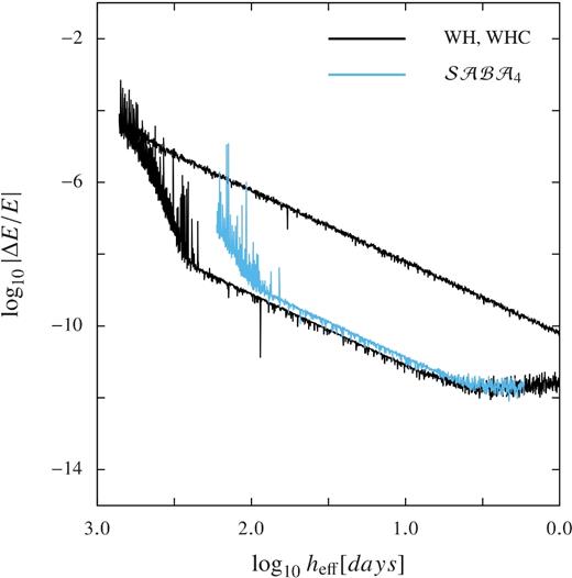
$The common logarithm of the absolute value of the relative energy error ΔE/E is plotted versus the common logarithm of the effective stepsize heff. The upper black curve is for the Wisdom–Holman method; the lower black curve is for the Wisdom–Holman method with the corrector. The blue curve is for the ${\cal SABA}_4$ method.$

Figure 1.

The common logarithm of the absolute value of the relative energy error ΔE/E is plotted versus the common logarithm of the effective stepsize h_eff. The upper black curve is for the Wisdom–Holman method; the lower black curve is for the Wisdom–Holman method with the corrector. The blue curve is for the |${\cal SABA}_4$| method.

Open in new tab Download slide

It is ironic that Laskar & Robutel (2001) dismiss the use of the corrector of Wisdom et al. (1996). They state ‘The use of such a procedure, especially when the solution is chaotic, is not clear’. The corrector was motivated by the averaging relationship between the integration variables and the actual variables. Yet, Laskar (1989) relied on averaging in his initial demonstration of the chaotic character of the motion of the Solar system!

Laskar & Robutel (2001) introduce a ‘corrector’ method to reduce the errors of their method. As mentioned, this corrector is not the same as the corrector introduced by Wisdom et al. (1996). The corrector of Laskar & Robutel (2001) is applied at every integration step. Taken literally, it is applied twice per integration step, but I have taken the liberty of optimizing the method by combining the two adjacent corrector steps. I find that the |${\cal SABAC}_4$| method is about a factor of 5.180 times slower than the Wisdom–Holman method. By contrast, the kernel method of Wisdom et al. (1996) is about a factor of 1.615 times slower than the Wisdom–Holman method. The results are reported in Fig. 2. One can see that the dynamical systems kernel method outperforms the method of Laskar & Robutel (2001). One can also see that the methods are reaching the limit of the numerical precision on the lower right side of the figure. I will address this issue in the next comparison.

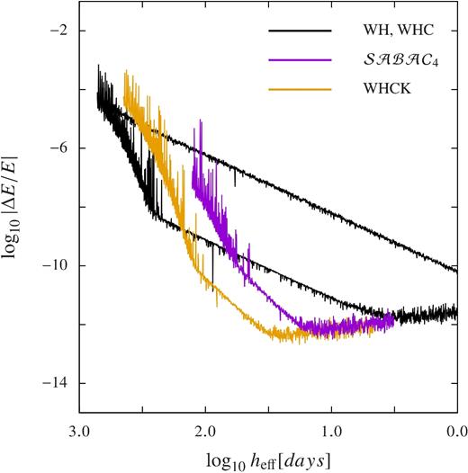
$The common logarithm of the absolute value of the relative energy error ΔE/E is plotted versus the common logarithm of the effective stepsize heff. The two black curves are again the Wisdom–Holman method and the Wisdom–Holman method with corrector. The purple curve is for the ${\cal SABAC}_4$ method. Considerable computer time must be expended before the large stepsize transient is passed. The orange curve is for the Wisdom–Holman method with the kernel and corrector. The kernel method is useable at a larger effective stepsize.$

Figure 2.

The common logarithm of the absolute value of the relative energy error ΔE/E is plotted versus the common logarithm of the effective stepsize h_eff. The two black curves are again the Wisdom–Holman method and the Wisdom–Holman method with corrector. The purple curve is for the |${\cal SABAC}_4$| method. Considerable computer time must be expended before the large stepsize transient is passed. The orange curve is for the Wisdom–Holman method with the kernel and corrector. The kernel method is useable at a larger effective stepsize.

Open in new tab Download slide

The limitation due to finite precision calculations is easily remediated at little cost. I use the method of compensated summation (Kahan 1965). I keep all the state variables as pairs of high and low parts of the variable (in ordinary double precision). Each time these state variables are modified, I add in the change using compensated summation. Define |$\hat{f}$| and |$\hat{\dot{g}}$| through |$f = 1 + \hat{f}$|⁠, and |$\dot{g} = 1 + \hat{\dot{g}}$|⁠. Assume that x and |${\boldsymbol v}$| are state variables consisting of a high and a low part. The high part (the most significant part) is extracted with the function |${\cal H}$|⁠. Let ⊕ be the addition operator using compensated summation. After one Kepler step, the new state variables are

\begin{eqnarray} {\boldsymbol x}^{\prime } &=& {\boldsymbol x} {\hbox{$\oplus $}} ((\hat{f} {\cal H}({\boldsymbol x})) {\hbox{$\oplus $}} (g {\cal H}({\boldsymbol v}))) \nonumber \\ {\boldsymbol v}^{\prime } &=& {\boldsymbol v} {\hbox{$\oplus $}} ((\hat{\dot{f}} {\cal H}({\boldsymbol x})) {\hbox{$\oplus $}} (\hat{\dot{g}} {\cal H}({\boldsymbol v}))). \end{eqnarray}

(28)

The f and g functions are computed with ordinary double precision. In a similar manner, I computed the kicks in ordinary double precision but modify the state using compensated summation.

Laskar & Robutel (2001) did not use this trick. Instead, they reported some results with complete quadruple precision calculations. I have taken the liberty of modifying the |${\cal SABAC}_4$| method to use compensated summation. I have also modified the kernel method. For the latter, I have applied both correctors. The results are shown in Fig. 3. One can see that both methods reach a relative error of order 10⁻¹⁴ in these 5.5 million year integrations. But the kernel method of Wisdom et al. (1996) reaches this level of error with less work.

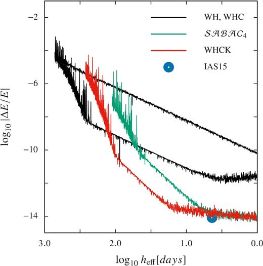
$The common logarithm of the absolute value of the relative energy error ΔE/E is plotted versus the common logarithm of the effective stepsize heff. The two black curves are again the Wisdom–Holman method and the Wisdom–Holman method with corrector. They are there for reference; I have not use compensated summation in either. The green curve is for the ${\cal SABAC}_4$ method extended here to use compensated summation. The red curve is for the kernel method (Wisdom et al. 1996). The kernel method is useable at a larger effective stepsize. The centre of the blue dot exhibits the results for the IAS15 variable stepsize integrator.$

Figure 3.

The common logarithm of the absolute value of the relative energy error ΔE/E is plotted versus the common logarithm of the effective stepsize h_eff. The two black curves are again the Wisdom–Holman method and the Wisdom–Holman method with corrector. They are there for reference; I have not use compensated summation in either. The green curve is for the |${\cal SABAC}_4$| method extended here to use compensated summation. The red curve is for the kernel method (Wisdom et al. 1996). The kernel method is useable at a larger effective stepsize. The centre of the blue dot exhibits the results for the IAS15 variable stepsize integrator.

Open in new tab Download slide

The centre of the large blue dot in Fig. 3 is the error of IAS15 for the same problem. The integrator IAS15 is a high-order variable stepsize integrator that selects its own stepsize (Rein & Spiegel 2014). In this case, the stepsize oscillates around 70–80 d. It also uses compensated summation to reduce error. To compute h_eff, I averaged the stepsize used (to find 75.17 d) and then divided by the ratio of the computing time to that of the Wisdom–Holman method. The kernel method, augmented with compensated summation, reaches a comparable error for the same h_eff.

It is interesting to note that the error continues to decline as the stepsize decreases even after the numerical floor is reached. This contrasts with the behaviour found in Fig. 2, where the error grows as the stepsize is decreased once the numerical floor is reached. Evidently, numerical error is a complicated process!

In billion year integrations of the outer planets, I find that when using WHC the energy error at large stepsizes does not appear to grow. Any growth of error is masked by oscillatory terms. At small stepsizes, the energy error grows irregularly, approximately as the square root of time. This is also true of the kernel method, whether or not compensated summation is used. Thus, these methods, which use the unbiased Kepler solver of Wisdom & Hernandez (2015), obey ‘Brouwer's law’ (Rein & Spiegel 2014).

6 CONCLUSIONS

The original method of Wisdom & Holman (1991), with the improvements of Wisdom et al. (1996) and the explicit implementation of the kernel method reported here, appears to be pretty much optimal for studying the evolution of regular planetary systems such as the motion of the outer planets. These methods can be used in either a ‘qualitative mode’ at large stepsizes with just the corrector, or in a high-accuracy mode with the kernel and associated correctors.

Acknowledgements

I thank Scott Tremaine, Hanno Rein, and Dan Tamayo for helpful remarks.

REFERENCES

Chirikov

B.

,

1979

,

Phys. Rep.

,

52

,

263

Crossref

Search ADS

Contopoulos

G.

,

Polymilis

C.

,

1987

,

Physica D

,

24

,

328

Crossref

Search ADS

Forest

E.

,

Ruth

R.

,

1990

,

Physica D

,

43

,

105

Crossref

Search ADS

Kahan

W.

,

1965

,

Commun. ACM

,

8

,

40

Crossref

Search ADS

Laskar

J.

,

1989

,

Nature

,

338

,

237

Crossref

Search ADS

Laskar

J.

,

Robutel

P.

,

2001

,

Celest. Mech. Dyn. Astron.

,

80

,

39

Crossref

Search ADS

Laskar

J.

,

Robutel

P.

,

Joutel

F.

,

Gastineau

M.

,

Correia

A.

,

Levrard

B.

,

2004

,

A&A

,

428

,

261

Crossref

Search ADS

Laskar

J.

,

Fienga

A.

,

Gastineau

M.

,

Manche

H.

,

2011

,

A&A

,

532

,

A89

Crossref

Search ADS

Rein

H.

,

Spiegel

D.

,

2014

,

MNRAS

,

446

,

1421

Rein

H.

,

Tamayo

D.

,

2015

,

MNRAS

,

452

,

376

Crossref

Search ADS

Saha

P.

,

Tremaine

S.

,

1992

,

AJ

,

104

,

1633

Crossref

Search ADS

Sussman

G. J.

,

Wisdom

J.

,

1992

,

Science

,

257

,

56

Crossref

Search ADS

PubMed

Sussman

G. J.

,

Wisdom

J.

,

2015

,

Structure and Interpretation of Classical Mechanics

, 2nd edn.

MIT Press

,

Cambridge, MA

Google Scholar

Google Preview

OpenURL Placeholder Text

WorldCat

Tittemore

W.

,

Wisdom

J.

,

1988

,

Icarus

,

74

,

172

Crossref

Search ADS

Wisdom

J.

,

1982

,

AJ

,

87

,

577

Crossref

Search ADS

Wisdom

J.

,

Hernandez

D. M.

,

2015

,

MNRAS

,

453

,

3015

Crossref

Search ADS

Wisdom

J.

,

Holman

M.

,

1991

,

AJ

,

102

,

1528

Crossref

Search ADS

Wisdom

J.

,

Holman

M.

,

1992

,

AJ

,

104

,

2022

Crossref

Search ADS

Wisdom

J.

,

Holman

M.

,

Touma

J.

,

1996

,

Fields Inst. Com.

,

10

,

217

Google Scholar

Google Preview

OpenURL Placeholder Text

WorldCat

Yoshida

H.

,

1990

,

Phys. Lett. A

,

150

,

262

Crossref

Search ADS

Yoshida

H.

,

1993

,

Celest. Mech. Dyn. Astron.

,

56

,

27

Crossref

Search ADS

APPENDIX

The strategy of Wisdom et al. (1996) was to start with the Hamiltonian governing the evolution of the system under study and transform this into the integrator Hamiltonian plus error terms through a series of canonical transformations. In this appendix, the strategy is reversed. I start with the Hamiltonian for the integrator and show that through canonical transformations this can be transformed into the Hamiltonian under study, plus some error terms. The two approaches are equivalent.

Let

\begin{equation} H = H_A + \epsilon H_B \end{equation}

(A1)

be the Hamiltonian under study.

Following Wisdom & Holman (1991), high-frequency terms are added to the Hamiltonian so that the system becomes locally integrable. The Hamiltonian for the integrator is

\begin{equation} H_M = H_A + \epsilon H_B + \epsilon \widetilde{H}_B, \end{equation}

(A2)

where

\begin{equation} \widetilde{H}_B = H_B \sum _{n \ne 0} \cos (n \Omega t). \end{equation}

(A3)

The Hamiltonian can be written in terms of periodic δ functions:

\begin{equation} H_M = H_A + 2 \pi \delta _{2 \pi } (\Omega t) H_B. \end{equation}

(A4)

The stepsize is h = 2π/Ω.

A Lie transform is performed to transform the integrator Hamiltonian into the actual Hamiltonian. In the extended phase space the integrator Hamiltonian is

\begin{equation} H^{\prime }_M = T + H_A + \epsilon H_B + \epsilon \widetilde{H}_B, \end{equation}

(A5)

where T is the momentum conjugate to time t. With the Lie generator W, the transformed Hamiltonian is

\begin{eqnarray} {\rm e}^{\epsilon L_W} H^{\prime }_M &=& (T + H_A) + \epsilon L_W (T + H_A) \nonumber \\ && +\, (1/2) \epsilon ^2 L^2_W (T + H_A) + \cdots \nonumber \\ && +\, \epsilon H_B + \epsilon ^2 L_W H_B + \cdots \nonumber \\ && +\, \epsilon \widetilde{H}_B + \epsilon ^2 L_W \widetilde{H}_B + \cdots . \end{eqnarray}

(A6)

The Lie derivative L_W is defined through L_WH = {H, W}, where the curly bracket indicates Poisson bracket.

The condition that the high-frequency terms are eliminated at first order in ε is

\begin{equation} L_W (T + H_A) + \widetilde{H}_B = 0. \end{equation}

(A7)

Using this, the extended Hamiltonian after the transformation is

\begin{eqnarray} {\rm e}^{\epsilon L_W} H^{\prime }_M &=& T + H_A + \epsilon H_B + (1/2) \epsilon ^2 L_W \widetilde{H}_B\nonumber\\ &&+\, \epsilon ^2 L_W H_B + \cdots . \end{eqnarray}

(A8)

To solve equation (A7) for the generator W, introduce E_n(τ) with the property E_n(τ) = DE_n + 1(τ). With E₀(τ) = 2πδ_2π(τ) − 1, the E_n for n > 0 are polynomials in the interval 0 < τ < 2π, and periodically extended. They are chosen to have zero average. Recognizing that |$\widetilde{H}_B = H_B E_0(\Omega t)$|⁠, the generator that solves equation (A7) is

\begin{equation} W = \sum _{k>0} \frac{(-1)^k L^{k-1}_{H_A} H_B}{\Omega ^k} E_k(\Omega t), \end{equation}

(A9)

as may be verified by substitution. (The k term of |$-L_{H_A} W$| cancels the k + 1 term of − ∂_tW. After these cancellations, the k = 1 term of − ∂_tW is left, and this cancels the H_BE₀(Ωt) term.) The E_n polynomials can be written in terms of the Bernoulli polynomials (Wisdom et al. 1996):

\begin{equation} E_n(\tau ) = - \frac{(2\pi )^n}{n!} B_n(\tau /(2\pi )). \end{equation}

(A10)

The first few Bernoulli polynomials are B₁(x) = x − (1/2), B₂(x) = x² − x + (1/6), B₃(x) = x³ − (3/2)x² + (1/2)x, and so on. So the generator may also be written as

\begin{equation} W = \sum _{k>0} (-1)^k (h)^k L^{k-1}_{H_A} H_B B_k(t/h). \end{equation}

(A11)

This is the generator that transforms away the high-frequency terms in the integrator Hamiltonian. The resulting canonical transformation is the ‘symplectic corrector’ of Wisdom et al. (1996). Notice that the corrector can be applied at any time t. The correction is smallest though when t = h/2 (halfway between the delta functions), because the first term, proportional to B_B(t/h), is zero there. This is one motivation for using the ‘leap frog’. Truncating the series at some chosen order, the canonical transformation may be written in terms of evolutions generated individually by H_A and H_B. See Wisdom et al. (1996) for details.

Notice that the momentum conjugate to time, T, appeared in only one place; it was added to the Hamiltonian to make the transition to the extended phase space. So if we perform the Lie transform with respect to W of any function of the original phase space coordinates, then there are no derivatives with respect to t (because T does not appear). In these cases, we may treat t as a parameter of the transformation. That is, it does not matter whether we assign t a value before or after the transformation. So having gone to the extended phase to determine W, we can return to the original phase space with t being a parameter. A convenient choice is t = h/2, and we obtain the corrector for the leap frog. It no longer depends on t and is only useful for transforming functions of the phase space coordinates midway between the delta functions.

To extend the integrator to higher order, examine the error terms in equation (A8). They are of two types: those involving |$L_W \widetilde{H}_B$| and those involving L_WH_B. Let us first ignore the L_WH_B terms, and consider only those involving |$\widetilde{H}_B$|⁠. Remember that we can write |$L_W \widetilde{H}_B = L_W H_B E_0(\Omega t)$|⁠. Let us perform a second Lie transform with the generator W₂ to eliminate these terms. The transformed integrator Hamiltonian is

\begin{eqnarray} T &+& H_A + \epsilon H_B + \epsilon ^2(L_{W_2} (T + H_A) + (1/2) L_W H_B \nonumber\\ &&\times\,E_0(\Omega t)+ L_W H_B) + \cdots . \end{eqnarray}

(A12)

So we can eliminate the |$L_W \widetilde{H}_B$| terms by solving

\begin{equation} L_{W_2} (T + H_A) + (1/2) L_W H_B E_0(\Omega t) = 0, \end{equation}

(A13)

for W₂. This looks just like equation (A7), except that H_B in that equation is replaced by (1/2)L_WH_B here. So, we could try to write down the solution by making that substitution:

\begin{equation} W_2 = \sum _{k>0} \frac{(-1)^k L^{k-1}_{H_A} ((1/2) L_W H_B)}{\Omega ^k} E_k(\Omega t). \end{equation}

(A14)

Substituting this into equation (A13), we find that most terms cancel as before. However, there are some extra terms that do not cancel because W is explicitly time dependent. When calculating ∂_tW₂, the product rule generates terms proportional to ∂_tW. These are generally non-zero, for arbitrary t. But for the leap frog, with t = h/2, the extra terms are zero. Note that B_n(1/2) = 0 for odd n. So for the leap frog, the only non-zero terms in W have even k. Then the extra terms are all proportional to B_n(1/2) for odd n, and thus are zero. Thus, equation (A14) is indeed the expression for W₂, but it only works for t = h/2.

Download all slides

Month:	Total Views:
November 2017	22
December 2017	18
January 2018	27
February 2018	4
March 2018	12
April 2018	15
May 2018	6
June 2018	7
July 2018	3
August 2018	9
September 2018	4
October 2018	7
November 2018	8
December 2018	8
January 2019	2
February 2019	1
March 2019	5
April 2019	5
May 2019	6
July 2019	9
August 2019	20
September 2019	10
October 2019	8
November 2019	3
December 2019	2
January 2020	5
February 2020	2
March 2020	3
June 2020	10
July 2020	16
August 2020	1
September 2020	4
November 2020	3
December 2020	2
January 2021	3
February 2021	1
March 2021	16
April 2021	11
May 2021	5
June 2021	1
July 2021	3
August 2021	4
September 2021	4
October 2021	7
November 2021	10
December 2021	12
January 2022	5
February 2022	9
March 2022	6
April 2022	14
May 2022	2
June 2022	6
July 2022	10
August 2022	7
September 2022	16
October 2022	6
November 2022	6
December 2022	12
January 2023	7
February 2023	3
March 2023	15
April 2023	7
May 2023	2
June 2023	6
July 2023	8
August 2023	13
September 2023	2
October 2023	19
November 2023	23
December 2023	27
January 2024	9
February 2024	6
March 2024	4
April 2024	5
May 2024	10
June 2024	5
July 2024	11
August 2024	13
September 2024	6
October 2024	12
November 2024	10
December 2024	7
January 2025	4
February 2025	7
March 2025	11
April 2025	11
May 2025	7

Article Contents

The dynamical systems approach to numerical integration

Abstract

1 INTRODUCTION

2 SOME BACKGROUND

3 HIGHER ORDER INTEGRATORS

4 CONTRASTING THE DYNAMICAL SYSTEMS APPROACH TO THE LIE SERIES APPROACH

5 COMPARISONS

6 CONCLUSIONS

Acknowledgements

REFERENCES

APPENDIX

Citations

Views

Altmetric

Email alerts

Astrophysics Data System

Citing articles via

Latest

Most Read

Most Cited

Article Contents

The dynamical systems approach to numerical integration

Abstract

1 INTRODUCTION

2 SOME BACKGROUND

3 HIGHER ORDER INTEGRATORS

4 CONTRASTING THE DYNAMICAL SYSTEMS APPROACH TO THE LIE SERIES APPROACH

5 COMPARISONS

6 CONCLUSIONS

Acknowledgements

REFERENCES

APPENDIX

Citations

Views

Altmetric

Email alerts

Astrophysics Data System

Citing articles via

Latest

Most Read

Most Cited

This Feature Is Available To Subscribers Only