Vortices and the saturation of the vertical shear instability in protoplanetary discs

Latter, Henrik N; Papaloizou, John

doi:10.1093/mnras/stx3031

Abstract

If sufficiently irradiated by its central star, a protoplanetary disc falls into an equilibrium state exhibiting vertical shear. This state may be subject to a hydrodynamical instability, the ‘vertical shear instability’ (VSI), whose breakdown into turbulence transports a moderate amount of angular momentum while also facilitating planet formation, possibly via the production of small-scale vortices. In this paper, we show that VSI modes (a) exhibit arbitrary spatial profiles and (b) remain non-linear solutions to the incompressible local equations, no matter their amplitude. The modes are themselves subject to parasitic Kelvin–Helmholtz instability, though the disc rotation significantly impedes the parasites and permits the VSI to attain large amplitudes (fluid velocities ≲ 10 per cent the sound speed). This ‘delay’ in saturation probably explains the prominence of the VSI linear modes in global simulations. More generally, the parasites may set the amplitude of VSI turbulence in strongly irradiated discs. They are also important in breaking the axisymmetry of the flow, via the unavoidable formation of vortices. The vortices, however, are not aligned with the orbital plane and thus express a pronounced z-dependence. We also briefly demonstrate that the vertical shear has little effect on the magnetorotational instability, whereas magnetic fields easily quench the VSI, a potential issue in the ionized surface regions of the disc and also at larger radii.

hydrodynamics, instabilities, MHD, protoplanetary discs

1 INTRODUCTION

Large swathes of protoplanetary (PP) discs are too poorly ionized for the magnetorotational instability (MRI) to be active, at least as classically understood (Turner et al. 2014). In particular, their cold dense interior regions (between roughly 1 and 10 au) could be entirely laminar, though non-ideal MHD may produce large-scale fields and winds (Bai 2014; Lesur, Kunz & Fromang 2014; Simon et al. 2015). In the last 10–15 years this state of affairs has renewed interest in hydrodynamical routes to turbulence in these ‘dead zones’, and various weak instabilities have been uncovered (or rediscovered) that might operate there (Fromang and Lesur 2017). It is unlikely that any of these instabilities is particular widespread, nor the solution to the question of angular momentum transport, but under certain circumstances they could be important, especially for solid dynamics and planet formation.

We focus on the vertical shear instability (VSI), a process that, as it names suggests, exploits any vertical shear supported by the disc. Indeed, irradiated PP discs generally manifest baroclinic equilibria that exhibit gentle vertical variation in the rotation rate (Nelson, Gressel & Umurhan 2013; Barker and Latter 2015). The VSI is a close cousin of the Goldreich–Schubert–Fricke instability (GSFI; Goldreich and Schubert 1967; Fricke 1968), and is similarly centrifugal in nature. When stable stratification is included it is also double-diffusive, with instability restricted to lengthscales upon which thermal diffusion is strong (negating the stable entropy gradient) but viscosity is weak (thus unable to obstruct the unstable angular momentum gradient).

While the GSFI probably saturates at too low a level to be important in stars (James and Kahn 1970, 1971; see also Caleo, Balbus & Tognelli 2016), the VSI may have greater traction in astrophysical discs, even if the intensity of its saturated state remains uncertain, and no doubt depends on how forcibly the vertical shear is maintained. Unlike the GSFI, the VSI's non-linear evolution has been pursued almost solely in global simulations (Nelson, Gressel & Umurhan 2013; Stoll and Kley 2014; Richard, Nelson & Umurhan 2016; Stoll, Kley & Picogna 2017). These show the flow degenerating into small-scale turbulence near or upon the disc's surfaces, followed by the emergence of large-scale inertial waves with little vertical structure. While the former activity is probably the work of the local modes described by Boussinesq analyses (Urpin and Brandenburg 1998; Urpin 2003), the latter waves are global modes that are best captured in vertically stratified models (Nelson, Gressel & Umurhan 2013; Barker and Latter 2015; Lin and Youdin 2015; McNally and Pessah 2015). Interesting features that arise in some simulations are vortices, whose aspect ratios and lifetimes depend on the background gradients (Richard, Nelson & Umurhan 2016). Because of their potential impact on solid dynamics, it is important to understand the nature of vortex formation and its connection to general VSI saturation. This is the main topic of this paper.

We work within the convenient framework of Boussinesq hydrodynamics because it is especially responsive to analytical techniques. We first reveal important properties of the small-scale VSI modes, such as (a) they are non-linear solutions to the governing equations (and hence can achieve large amplitudes naturally), and (b) they can manifest arbitrary spatial profiles. This gives us confidence that our Boussinesq analysis adequately approximates some of the non-linear waves and other features appearing in global simulations. We also apply the linear theory to simple low-mass PP disc models, finding in particular that the VSI grows at near its maximum rate even at 1 au on scales of order 10⁻²H or less (where H is the disc scale height). Larger scale body modes may be subdominant here, but small-scale VSI turbulence is still viable.

Because the non-linear VSI modes exhibit significant shear and vorticity extrema, they are subject to Kelvin–Helmholtz parasitic instability. As a consequence, small-scale vortices are a robust and unavoidable outcome of the VSI's evolution. The advent of both axisymmetric and non-axisymmetric parasites is delayed until the VSI achieves a relatively large amplitude, characterized by a Rossby number greater than 1 (velocities between 1 and 10 per cent the sound speed). Up to that point the axisymmetric parasites are stabilized by the disc's radial angular momentum gradient, while the non-axisymmetric parasites are sheared out before they get large. These two effects explain why the linear VSI modes feature so prominently in global simulations, at least initially.

More generally, the parasites may set the level of VSI turbulence, but only if the vertical shear is vigorously enforced by the stellar radiation field. If the VSI is especially efficient vis-a-vis the stellar driving, the saturated state will be low amplitude and controlled by the competition between the VSI and the driving, not the parasites. One could also imagine intermediate scenarios when all the physical processes are important.

We finally include a short section exploring the influence of MHD. Because of the vertical shear, magnetic equilibria have to be constructed carefully in order to satisfy Ferraro's law. We find that sufficiently strong magnetic fields stabilize the VSI: when ideal MHD holds and the average vertical plasma beta (β) is less than roughly (R/H)² ∼ 400 then no VSI modes of any length can grow. But the critical β is far higher for short-scale modes, and this poses a problem for the VSI in the relatively well ionized upper layers of PP discs – locations in which it is thought to be most prevalent. It may also be an issue at larger radii throughout the vertical column. In contrast, vertical shear has no impact on the fastest growing magnetorotational modes.

The paper plan is as follows. In Section 2 we revisit the VSI analysis in a Boussinesq local model, showing that the linear modes are also non-linear solutions and calculating both axisymmetric and non-axisymmetric examples, growth rates, and stability criteria. A short subsection applies these results to simple low-mass disc models and makes some comparison with previous work. Section 3 analyses the parasitic instabilities that may attack the non-linear VSI modes, examining axisymmetric and non-axisymmetric parasites separately and for different limiting amplitudes of the underlying VSI. Section 4 presents a relatively brief generalization to MHD, in which the MRI makes an appearance. We draw our conclusions in Section 5.

2 THE VERTICAL SHEAR INSTABILITY

2.1 Equations of incompressible hydrodynamics

In this section we describe the VSI in the framework of incompressible hydrodynamics, a model that successfully represents flows that are subsonic and which support only small thermodynamic variations (as is the case for shear/centrifugal instabilities like the VSI). Consequently, lengthscales are assumed to be much less than the disc scale height, and global disc features are not described properly. However, the disc's large-scale vertical shear can be incorporated into this model in a straightforward and consistent way as shown by Latter and Papaloizou (2017). At this stage vertical stratification (i.e. buoyancy), radiative cooling, and viscous diffusion are neglected. This need not be a problem for the VSI, however, as there is often a range of lengthscales between the vast gulf separating the viscous scales (∼10 km) and the stratification scale (∼H), within which thermal diffusion (or cooling) dominates and ‘cancels out’ the latter stabilizing effect. The system on these scales neither feels viscosity, stratification, nor thermal diffusion itself. In Appendix A we reproduce an analysis with the omitted physics to show that our main results are unaltered.

In addition, we adopt the shearing sheet formalism, whereupon a small patch of the PP disc centred at R = R₀ and Z = Z₀ ≠ 0, and orbiting with frequency Ω₀ = Ω(R₀, Z₀) is described using a corotating Cartesian reference frame. In it x, y, and z represent the local radial, azimuthal, and vertical directions, with their origin the centre of the box.

The equation of motion in our incompressible, vertically shearing, local model is

\begin{equation} \mathrm{\partial} _t\boldsymbol {u}+ \boldsymbol {u}\cdot \nabla \boldsymbol {u}= -\frac{1}{\rho }\nabla P -2\Omega \boldsymbol {e}_{z}\times \boldsymbol {u}+ \Omega ^2 (3x +2z q) \boldsymbol {e}_{x}, \end{equation}

(1)

where |$\boldsymbol {u}$| is fluid velocity, ρ is the constant density, P is the pressure, and

\begin{equation*} q= -R_0\frac{\mathrm{\partial} \ln \Omega }{\mathrm{\partial} z} \end{equation*}

evaluated at the point R = R₀, Z = Z₀ (see Latter and Papaloizou 2017). Finally, the fluid velocity satisfies the incompressibility requirement:

\begin{equation} \nabla \cdot \boldsymbol {u}=0. \end{equation}

(2)

The parameter q quantifies the degree of vertical shear at the shearing sheet location, and is generally small; from the thermal wind equation comes the estimate q ∼ (H/R) (Barker and Latter 2015). Note that as Z₀ increases, so usually will q. The angular momentum gradient ∇(R²Ω) in the shearing sheet is the vector

\begin{equation} \nabla \ell = \frac{1}{2}R_0\Omega _0(\boldsymbol {e}_{x}-2q\boldsymbol {e}_{z}), \end{equation}

(3)

which points predominantly in the radial direction.

One of the attractions of these equations is that they are controlled by a single parameter q, and have no natural lengthscale: the outer scale is taken to infinity, while the viscous scale is taken to zero. This, of course, makes them difficult to directly apply to real systems – but makes analytical progress much easier.

2.2 General non-linear perturbations

The set (1) and (2) admits the steady equilibrium state of linear radial and vertical shear:

\begin{equation} \boldsymbol {u}= \boldsymbol {u}_0 =-\frac{1}{2}\Omega _0(3x + 2 z q)\boldsymbol {e}_{y}, \qquad P=P_0, \end{equation}

(4)

where P₀ is a constant. This equilibrium is then perturbed by disturbances |$\boldsymbol {u}_1$| and P₁, which must obey

\begin{eqnarray} \mathrm{\partial} _t \boldsymbol {u}_1 +\boldsymbol {u}_0\cdot \nabla \boldsymbol {u}_1 + \boldsymbol {u}_1\cdot \nabla \boldsymbol {u}_1 &=& -\frac{1}{\rho }\nabla P_1 -2\Omega _0 \boldsymbol {e}_{z}\times \boldsymbol {u}_1 \nonumber \\ &&+\, \Omega _0 \left(\frac{3}{2}u_{1x} + q u_{1z}\right)\boldsymbol {e}_{y}, \end{eqnarray}

(5)

and |$\nabla \cdot \boldsymbol {u}_1=0$|⁠.

We next introduce the wavevector |$\boldsymbol {k}(t)$|⁠, which is potentially a function of time, and construct the independent variable |$\xi = \boldsymbol {k}\cdot \boldsymbol {x}$|⁠. We also assume that our perturbations depend on ξ and t in the following way:

\begin{equation} \boldsymbol {u}_1= \bar{\boldsymbol {u}}(t) f(\xi ){\, } \qquad P_1= \bar{P}(t)\left(\int f(\xi ){\, }{\rm d}\xi \right), \end{equation}

(6)

where |$\bar{\boldsymbol {u}}$| and |$\bar{P}$| are functions to be determined, while f is an arbitrary differentiable function.

Using suffix notation, it is straightforward to show that the incompressibility condition becomes

\begin{equation} {}\boldsymbol {k}\cdot \bar{\boldsymbol {u}} = 0, \end{equation}

(7)

and thus the fluid is constrained to move perpendicularly to the vector |$\boldsymbol {k}$| (oscillations are transverse). But then

\begin{eqnarray*} (\boldsymbol {u}_1\cdot \nabla \boldsymbol {u}_1)_j = f\bar{u}_i \frac{\mathrm{\partial} f}{\mathrm{\partial} x_i}{\, }\bar{u}_j, = f\frac{{\rm d}f}{{\rm d}\xi }(k_i\bar{u}_i)\bar{u}_j = 0, \end{eqnarray*}

and the non-linear terms in the equation of motion vanish, a significant simplification. It also means that our perturbations are concurrently linear and non-linear solutions.

Turning next to the equation of motion, the pressure gradient term simplifies in the following way:

\begin{equation*} \nabla P_1 = \bar{P}\nabla \left(\int f {\, }{\rm d}\xi \right)= \bar{P}{\, }f{\, }\nabla \xi = \bar{P}{\, }f{\, }\boldsymbol {k}, \end{equation*}

and the remaining terms in the advective derivative become

\begin{equation*} \mathrm{\partial} _t\boldsymbol {u}_1 + \boldsymbol {u}_0\cdot \nabla \boldsymbol {u}_1 = f\mathrm{\partial} _t\bar{\boldsymbol {u}}+\bar{\boldsymbol {u}}\frac{{\rm d}f}{{\rm d}\xi } \left[ x_i \mathrm{\partial} _t k_i-\left(\frac{3}{2} x + qz\right)\Omega _0 k_y \right]. \end{equation*}

Up to now the form of |$\boldsymbol {k}$| has been left free. We next select a form so that the square bracketed expression above is zero. This yields ODEs for the components of |$\boldsymbol {k}$|⁠:

\begin{eqnarray*} \frac{{\rm d}k_x}{{\rm d}t} =\frac{3}{2}\Omega _0 k_y, \quad \frac{{\rm d}k_y}{{\rm d}t} =0, \quad \frac{{\rm d}k_z}{{\rm d}t} =q\Omega _0 k_y. \end{eqnarray*}

Immediately we see that k_y is a constant, while k_x and k_z increase linearly with time:

\begin{eqnarray} k_x = k_x^0 + \frac{3}{2}\Omega _0 k_y t, \end{eqnarray}

(8)

\begin{eqnarray} k_z = k_z^0 + q\Omega _0 k_y t, \end{eqnarray}

(9)

where |$k_x^0$| and |$k_z^0$| are constants. Thus non-axisymmetric disturbances possess wavevectors that are sheared out by the differential rotation in r and z. Ultimately |$\boldsymbol {k}$| is perpendicular to surfaces of constant Ω; i.e. k_x/k_z → 3/(2q) as t → ∞ (Balbus et al. 2009; Balbus and Schaan 2012). Our solutions may then be understood as (doubly) shearing waves but with arbitrary spatial profiles: they need not take the form of sinusoids familiar from previous work (cf. Johnson and Gammie 2005; Hawley and Balbus 2006; Balbus and Schaan 2012; Caleo and Balbus 2016; Caleo, Balbus & Tognelli 2016), and yet they still remain non-linear solutions to the governing equations. This property has nothing to do with the vertical shear, of course, but issues directly from the incompressible shearing box approximation.

Now every term in equation (5) is proportional to f. The spatial variable hence can be eliminated, leaving a vector ODE in terms of time:

\begin{eqnarray} \frac{{\rm d}\bar{\boldsymbol {u}}}{{\rm d}t}= -\boldsymbol {k}\frac{\bar{P}}{\rho }-2\Omega _0\boldsymbol {e}_{z}\times \bar{\boldsymbol {u}} +\Omega _0\left(\frac{3}{2}\bar{u}_x +q \bar{u}_z\right)\boldsymbol {e}_{y}. \end{eqnarray}

(10)

By taking the scalar product of (10) with |${\boldsymbol k}$| and making use of the time derivative of the incompressibility condition we obtain an expression for P/ρ in the form

\begin{equation*} \frac{P}{\rho }=\frac{\Omega _0}{k^2}\left(k_y \bar{u}_x+2k_x \bar{u}_y +2q k_y\bar{u}_z\right), \end{equation*}

with |$k^2= k_x^2+k_y^2+k_z^2.$| Equation (10) can be reduced to a single scalar ODE of third order. In the special case of q = 0 this reduces to second order and can be solved in terms of special functions (see for example, Johnson and Gammie 2005).

In order to obtain complete solutions in the non-axisymmetric case the system must be solved numerically. However, we can obtain the perturbations’ asymptotic behaviour as t → ∞ analytically which is sufficient to assess their ultimate stability. We find that for large t ≳ 1/(q²Ω₀), |$\bar{\boldsymbol {u}} \sim t^\alpha {\rm exp}\left(\frac{4}{3}{\rm i}q\Omega _0 t\right)$|⁠, where

\begin{equation*} \alpha = -\frac{1}{2} \pm \left(\frac{5k_z^0}{6k_y}-\frac{5q k_x^0}{9k_y}\right){\rm i}. \end{equation*}

Thus all non-axisymmetric modes decay algebraically, while oscillating on an intermediate time-scale ∼1/(qΩ₀). Details of this calculation are provided in Appendix B.

2.3 The axisymmetric VSI

The above scaling fails when the disturbances are axisymmetric, k_y = 0. In this case |$\boldsymbol {k}$| is a constant and |$\bar{\boldsymbol {u}}$| and |$\bar{P}$| can be decomposed into temporal Fourier modes, greatly easing the analysis. We set them proportional to exp(st), where s is a growth rate, and the perturbation equations become algebraic:

\begin{eqnarray} s\bar{u}_x = -\frac{1}{\rho }k_x \bar{P} + 2\Omega \bar{u}_y,\quad s\bar{u}_y=-\frac{1}{2}\Omega \bar{u}_x + q\Omega \bar{u}_z, \end{eqnarray}

(11)

\begin{eqnarray} s\bar{u}_z = -\frac{1}{\rho }k_z \bar{P}, &\quad k_x\bar{u}_x + k_z\bar{u}_z = 0. \end{eqnarray}

(12)

Eliminating the dependent variables obtains the dispersion relation

\begin{equation} s^2 = -\frac{k_z^2}{k^2}\Omega ^2\left(1+ 2q \frac{k_x}{k_z} \right) =-\frac{k_z}{k^2}\Omega ^2\left[\boldsymbol {k}\cdot (\nabla \ell )^\perp \right], \end{equation}

(13)

where |$(\nabla \ell )^\perp = 2q\boldsymbol {e}_{x}+\boldsymbol {e}_{z}$|⁠, and is thus a vector perpendicular to the angular momentum gradient [cf. equation (3)]. This relation reproduces equation (31) in Urpin and Brandenburg (1998) and equation (36) in Nelson, Gressel & Umurhan (2013). Instability is assured whenever q ≠ 0 for perturbations with suitably oriented wavevectors:

\begin{equation} q\frac{k_x}{k_z} < -\frac{1}{2}. \end{equation}

(14)

Marginal stability, s = 0, occurs when |$\boldsymbol {k}\rightarrow \boldsymbol {e}_{x}$| or when |$\boldsymbol {k}$| is parallel to the angular momentum gradient ∇ℓ (Knobloch and Spruit 1982), with growth limited to wavevector orientations lying between |$\boldsymbol {e}_{x}$| and ∇ℓ. Because ∇ℓ is almost radial, the VSI is thus restricted to a narrow arc of wavevector orientations, spanning an angle of only ≈2q above the radial axis.

There is no characteristic lengthscale in the governing equations, and so the growth rate can only depend on wavevector orientation. Viscosity or vertical structure will introduce a lengthscale dependence. See Appendix A and Section 2.4 for more details. Because non-axisymmetric disturbances always tend to orient themselves along the gradient of Ω, i.e. k_x/k_z = 2/(3q), they becomes stable after some point in their evolution, and hence ultimately decay, as shown explicitly at the end of the last subsection.

The peak growth rate can be obtained by maximizing s over k_x/k_z. The critical k_x/k_z may be obtained from the quadratic

\begin{equation*} q(k_x/k_z)^2 + (k_x/k_z) - q =0. \end{equation*}

In the natural limit of small q, asymptotic solutions are k_x/k_z = q, −1/q. Only the latter yields a positive growth rate, and this corresponds to

\begin{equation} s \approx \Omega |q|, \end{equation}

(15)

in agreement with previous analyses (Urpin and Brandenburg 1998; Urpin 2003). Because q ≪ 1 the growth rate is considerably less than the orbital frequency, and fastest growth occurs when k_x/k_z ≈ −1/q, corresponding to disturbances that are radially narrow and vertically elongated (as seen in numerical simulations).

2.4 Stratification, cooling, and viscosity

We now briefly summarize the full problem in which buoyancy, viscous diffusion, and cooling is included. In PP discs, the photon mean free path varies substantially: from a tiny fraction of H at 1 au, to greater than H at 100 au (e.g. Lin and Youdin 2015; Lesur and Latter 2016). As a consequence, radiative cooling takes different forms, depending on the age/mass of the disc, radial, and vertical location, and on the lengthscale of the perturbations. We mainly adopt the diffusion approximation, but are aware this is invalid for sufficiently short-scale perturbations at radii less than about 10 au, and for almost all perturbations at larger radii. The viscosity we employ is treated as molecular, though might also represent diffusion by weak pre-existing small-scale turbulence. It could also be a model for unavoidable grid diffusion in numerical simulations.

Two new parameters now appear, (a) the Richardson number n² = N²/Ω², where N is the vertical buoyancy frequency, and (b) the Prandtl number Pr = κ/ν where κ is thermal diffusivity and ν viscosity.

2.4.1 Main results

In Appendix A we derive a number of results and summarize them here. First we find that the analysis of Section 2.1–2.3 holds on a broad range of radial lengthscales λ

\begin{equation} \sqrt{\frac{1}{q}\frac{\nu }{\Omega }}{\, } \ll {\, } \lambda {\, } \ll {\, } \sqrt{\frac{q}{n^2}\frac{\kappa }{\Omega }}. \end{equation}

(16)

Perturbations within this range are sufficiently long so that viscosity is weak, but sufficiently short so that the stabilizing buoyancy force can be negated by thermal diffusion. Note that the vertical lengthscale of the modes will be 1/q ∼ R₀/H longer than λ. The existence of this range is assured if

\begin{equation} {\rm Pr} \lesssim \frac{q^2}{n^2} \sim \left(\frac{H}{r}\right)^2\left(\frac{\Omega }{N}\right)^2. \end{equation}

(17)

Equation (13) provides a good estimate of the growth rate on this range. An important thing to note is that, within the confines of the Boussinesq model, the VSI lengthscales are set by the diffusivities. This has to be, because the instability is double diffusive in nature.

On shorter scales the diffusion approximation breaks down and we may replace it with Newtonian cooling. Typically, the transition between these two cooling regimes occurs within the plateau of maximum growth, described above. The wavenumber of the transition can be estimated from either k ∼ 1/l_ph, where l_ph denotes the photon mean fee path, or simply |$k \sim 1/\sqrt{\tau \kappa }$|⁠, where τ is the Newtonian cooling time-scale. At the transition point the cooling rate, which had been increasing with k², hits the constant Newtonian ceiling. See Lin and Youdin (2015) for a detailed treatment of this transition.

As shown in Appendix A, maximum growth can be maintained in this regime when the cooling is sufficiently fast

\begin{equation} \Omega \tau \ll q\left(\frac{\Omega ^2}{N^2}\right). \end{equation}

(18)

A similar expression is obtained by Lin and Youdin (2015). Even if the cooling is slow, growth can be sustained but at a lower rate, with instability quenched only for exceedingly long cooling times

\begin{equation} \Omega \tau > \frac{q^2}{n^2}{\rm Re}, \end{equation}

(19)

where Re = H²Ω/ν is the Reynolds number.

2.4.2 Application to a low-mass disc

We now see how these estimates fare when applied to models of PP disc structure. Consider the less massive nebula used in Lesur and Latter (2016), in which the disc's surface density is |$\propto 140 R_{\rm {au}}^{-1}$| g cm⁻² and the temperature is equal to 280|$R_{\rm {au}}^{-1/2}$| K. Here R_au is disc radius in au. PP discs are moderately stratified, with n ≲ 1, and we set q ∼ H/R ∼ 0.05. Lesur and Latter (2016) also estimate the photon mean free path, which rises from a little over 10⁻⁴H at 1 au, to ∼10⁻²H at 10 au, before exceeding H at 100 au. Fluctuations with lengthscales below this cool at the Newtonian rate: less than 10⁻³ Ω⁻¹ for radii between 1 and 10 au, but rising to 5 × 10⁻² Ω⁻¹ at 100 au. Table 1 summarizes some of this information.

Table 1.

Open in new tab

Properties of a low-mass PP disc at three different radii. Here Σ is surface density, l_ph is photon mean path, and τ is the cooling rate for lengthscales less than l_ph. Here |$\lambda ^{\rm plat}_{\rm VSI}$| denotes the lengthscale below which the VSI achieves its maximum value (in the diffusion approximation). On lengthscales less than l_ph, however, the VSI can grow at its maximum level if τΩ ≪ 5 × 10⁻².

Radius	1 au	10 au	100 au
Σ/(gcm⁻²)	140	14	1.4
l_ph/H	10⁻⁴	10⁻²	>1
τΩ	10⁻⁴	≲ 10⁻³	10⁻²
\|$\lambda ^{\rm plat}_{\rm VSI} / H$\|	3 × 10⁻²	≲ 1	∼1

Radius	1 au	10 au	100 au
Σ/(gcm⁻²)	140	14	1.4
l_ph/H	10⁻⁴	10⁻²	>1
τΩ	10⁻⁴	≲ 10⁻³	10⁻²
\|$\lambda ^{\rm plat}_{\rm VSI} / H$\|	3 × 10⁻²	≲ 1	∼1

Table 1.

Open in new tab

Properties of a low-mass PP disc at three different radii. Here Σ is surface density, l_ph is photon mean path, and τ is the cooling rate for lengthscales less than l_ph. Here |$\lambda ^{\rm plat}_{\rm VSI}$| denotes the lengthscale below which the VSI achieves its maximum value (in the diffusion approximation). On lengthscales less than l_ph, however, the VSI can grow at its maximum level if τΩ ≪ 5 × 10⁻².

Radius	1 au	10 au	100 au
Σ/(gcm⁻²)	140	14	1.4
l_ph/H	10⁻⁴	10⁻²	>1
τΩ	10⁻⁴	≲ 10⁻³	10⁻²
\|$\lambda ^{\rm plat}_{\rm VSI} / H$\|	3 × 10⁻²	≲ 1	∼1

Radius	1 au	10 au	100 au
Σ/(gcm⁻²)	140	14	1.4
l_ph/H	10⁻⁴	10⁻²	>1
τΩ	10⁻⁴	≲ 10⁻³	10⁻²
\|$\lambda ^{\rm plat}_{\rm VSI} / H$\|	3 × 10⁻²	≲ 1	∼1

The plateau of maximum growth occurs for wavelengths roughly less than q^1/2n⁻¹Pe^−1/2H, where Pe = H²Ω/κ is the Peclet number. At 1 au we find that the plateau begins at a wavelength less than 3 × 10⁻²H, and thus the fastest growing modes are shortscale and well described by our Boussinesq model. The photon mean free path, on the other hand, is l_ph ∼ 10⁻⁴H and so the diffusion approximation holds for at least two decades in wavenumber upon which maximum growth is achieved. Below l_ph, however, the VSI will remain growing at the same maximum value until the viscous cut-off, this is because the Newtonian cooling rate τ easily satisfies (18).

At 10 au, we find that the plateau begins at a longer lengthscale ≲H, and thus the local model is a poor approximation on the long end of the range of maximum growth. At this location l_ph ∼ 10⁻² and the diffusion approximation still holds on this upper range, while the Newtonian cooling rate still satisfies (18).

At 100 au, l_ph > H and the diffusion approximation must be discarded entirely in favour of a Newtonian cooling prescription (Lin and Youdin 2015). Moreover, maximum growth is no longer possible because Ωτ ∼ 10⁻² ∼ q(Ω²/N²), and (18) no longer satisfied. At these radii the VSI begins to suffer, growing at a lower rate, in rough agreement with analogous calculations (Lin and Youdin 2015; Malygin et al. 2017).

To inspect how the VSI fares in more massive disc models the reader is directed to Lin and Youdin (2015) and Malygin et al. (2017). Due to the longer cooling times of these objects, the VSI is less prevalent. However, we do point out that short-scale VSI modes should not be neglected in these analyses. Though they may be inefficient at transporting angular momentum, or erasing the vertical shear, they are still perfectly good at generating vortices. And vortices need not be large-scale to do interesting things with solid particles.

2.5 Example solutions

In this subsection we present some numerical solutions describing the VSI's evolution. To get a better idea of how the unstratified axisymmetric mode depends on the orientation of its wavevector, we plot in Fig. 1 the growth rate s versus tan⁻¹(k_z/k_x), the angle the wavevector makes with respect to the x-axis. Quite clear is the extremely narrow range of angles available to the VSI, some 6° above the disc plane. Maximum growth, as shown earlier, occurs when k_x/k_z ≈ −1/q.

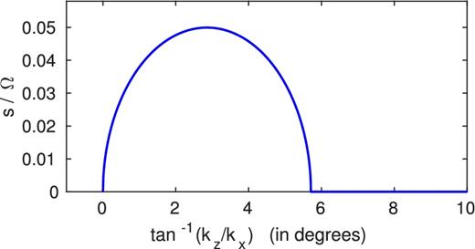
Growth rate of the axisymmetric VSI, as determined by equation (13) as a function of wavenumber orientation angle tan −1(kz/kx) as measured from the x-axis. The angle is given in degrees. Here q = −0.05 and we see that instability takes its maximum value ∼|q|Ω, while being restricted to a narrow arc of wavevector angles spanning only some 6°.

Figure 1.

Growth rate of the axisymmetric VSI, as determined by equation (13) as a function of wavenumber orientation angle tan ⁻¹(k_z/k_x) as measured from the x-axis. The angle is given in degrees. Here q = −0.05 and we see that instability takes its maximum value ∼|q|Ω, while being restricted to a narrow arc of wavevector angles spanning only some 6°.

Open in new tab Download slide

In Fig. 2 we plot the evolution of |$\bar{u}_x(t)$| for a non-axisymmetric VSI disturbance in time. The system of equations (10) was solved with a Runge–Kutta algorithm, for fiducial initial conditions corresponding to a leading wave at t = 0. Substantial growth occurs near Ωt ≈ 42.5, as the wave vector passes through the arc of axisymmetric growth (around k_x/k_z ≈ −1/q). Once the wavevector enters stable orientations, at later times, the disturbance decays as predicted, oscillating with a frequency ∼qΩ with an envelope going as t^−1/2.

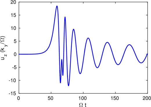
$Numerical solution to equation (10) for a non-axisymmetric disturbance with kx0/ky = −100, kz0/ky = 1, and initial condition $\bar{u}=(0.01,{\, }-0.01,{\, }0.01)$. Finally, q = −0.1.$

Figure 2.

Numerical solution to equation (10) for a non-axisymmetric disturbance with k_x0/k_y = −100, k_z0/k_y = 1, and initial condition |$\bar{u}=(0.01,{\, }-0.01,{\, }0.01)$|⁠. Finally, q = −0.1.

Open in new tab Download slide

Finally, in Fig. 3 we plot a representative dispersion relation for the axisymmetric VSI with stratification, viscosity, and thermal diffusion. Note the conspicuous plateau extending from roughly the thermal diffusion scale |$\sqrt{\kappa /\Omega }$| to the viscous cut-off some two orders of magnitude smaller. Upon the plateau, s takes almost the same value as in the inviscid unstratified situation, equation (13).

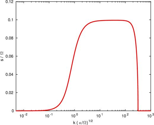
$Growth rate of the axisymmetric VSI when stratification, viscosity, and thermal diffusion are included. Parameters are q = −0.1, Pr = 10−6, n2 = 0.1, and kx/kz = 10. Here the viscous scale corresponds to kν ∼ 103, in units of $\sqrt{\Omega /\kappa }$, while the thermal diffusion scale is ∼1. The fastest growth occurs on a range of lengths between these limits, and here s is approximately the same as if there were no stratification, nor viscous and thermal diffusion.$

Figure 3.

Growth rate of the axisymmetric VSI when stratification, viscosity, and thermal diffusion are included. Parameters are q = −0.1, Pr = 10⁻⁶, n² = 0.1, and k_x/k_z = 10. Here the viscous scale corresponds to k_ν ∼ 10³, in units of |$\sqrt{\Omega /\kappa }$|⁠, while the thermal diffusion scale is ∼1. The fastest growth occurs on a range of lengths between these limits, and here s is approximately the same as if there were no stratification, nor viscous and thermal diffusion.

Open in new tab Download slide

3 KELVIN–HELMHOLTZ PARASITES

Because the VSI modes are non-linear solutions they can grow to arbitrarily large amplitudes, at least in principle. Before they grow too large, however, they will be attacked by secondary parasitic instability, especially if the spatial profile of the modes f(ξ) exhibits sufficient shear. As in similar problems (e.g. the MRI), the primary parasitic instability will be of Kelvin–Helmholtz type (Goodman and Xu 1994; Latter, Lesaffre & Balbus 2009; Pessah and Goodman 2009), which in the hydrodynamic context may lead to vortex formation. (In MHD, magnetic tension prevents the rolling up of vortex sheets.) In this section of the paper we explore how effective parasitic modes are and how associated vortices may arise.

We take the state of homogeneous vertical and radial shear, |$\boldsymbol {u}_0$| and P₀, given by equation (4) and then add to it an axisymmetric VSI mode, |$\boldsymbol {u}_1$| and P₁, given by equation (6). The VSI velocity field may be written as

\begin{eqnarray} \boldsymbol {u}_1= V{\, }\bar{\boldsymbol {u}}{\, }f(\xi ){\, }{\rm e}^{st}, \end{eqnarray}

(20)

where |$\bar{\boldsymbol {u}}$| is a constant eigenvector determined from equations (11) and (12), non-dimensionalized and normalized so that |$|\bar{\boldsymbol {u}}|=1$|⁠, and s is the growth rate, given by (13). Taking f(ξ) to be dimensionless and with a maximum value of order unity, the parameter V is then the characteristic velocity amplitude of the VSI mode at t = 0. It possesses units of speed. Because the solution is axisymmetric, the wavevector |$\boldsymbol {k}$| is a constant, which introduces the only lengthscale in the problem.

The key parameter in what follows is the amplitude of the VSI mode, V, which can only be expressed in terms of Ω/k. We regard the VSI mode to be of small amplitude if V ≪ Ω/k, of moderate amplitude if V ∼ Ω/k, and of large amplitude if V ≫ Ω/k. This motivates the introduction of the VSI's Rossby number Ro =kV/Ω, a proxy for the VSI amplitude.

The sum of the two fields, |$\boldsymbol {u}_0$| and |$\boldsymbol {u}_1$|⁠, we take to be our background, time varying, state. We next perturb this state with small disturbances, denoted by |$\boldsymbol {u}_2$| and P₂. The linearized equations for the disturbances are

\begin{eqnarray} \mathrm{\partial} _t\boldsymbol {u}_2 &-&\left(\frac{3}{2} x+ qz \right)\Omega {\, } \mathrm{\partial} _y \boldsymbol {u}_2 +\boldsymbol {u}_1\cdot \nabla \boldsymbol {u}_2 +(\boldsymbol {k}\cdot \boldsymbol {u}_2)\mathrm{\partial} _\xi \boldsymbol {u}_1 \nonumber \\ \hspace{14.22636pt}&&=\,-\frac{1}{\rho }\nabla P_2 -2\Omega \boldsymbol {e}_{z}\times \boldsymbol {u}_2 + \left(\frac{3}{2}\Omega u_{2x}+q\Omega u_{2z}\right)\boldsymbol {e}_{y} \end{eqnarray}

(21)

and

\begin{equation} \nabla \cdot \boldsymbol {u}_2=0. \end{equation}

(22)

These differ from the usual linearized equations for a homogeneous background of uniform shear because of the additional terms involving |$\boldsymbol {u}_1$|⁠. The equation of motion (21) depends explicitly on time (through |$\boldsymbol {u}_1$|⁠) and x and z, thus we cannot Fourier decompose the perturbation |$\boldsymbol {u}_2$| in any of these independent variables. As such equation (21) presents a considerable challenge to solve: it is a PDE in three variables. In the next two subsections we look at various limits in which the problem reduces to something more manageable. Subsequently, we collate these results and construct a theory for the destruction of VSI modes and the emergence of vortices from their breakdown.

3.1 Axisymmetric parasites

The first simplifying case we investigate assumes that the parasite is axisymmetric, so that |$\mathrm{\partial} _y\boldsymbol {u}_2=\mathrm{\partial} _yP_2=0$|⁠. This is not especially restrictive: for modest amplitudes of the background VSI (and parasitic growth rates of order Ω or less), axisymmetric parasites should be the most effective in overcoming their hosts. This is because non-axisymmetric disturbances are sheared out on their instability time-scale and only grow transiently: in their short window of growth they may fail to achieve sufficient amplitudes (Appendix B of Latter et al. 2010, and also Rembiasz et al. 2016).

When the parasites are axisymmetric, the spatial variables in (6) appear only via f’s dependence on |$\xi =\boldsymbol {k}\cdot \boldsymbol {x}=k_x x + k_z z.$| To exploit this fact, we introduce the coordinate transformation (x, z) → (ζ, η), where the ζ coordinate axis points in the direction of |$\boldsymbol {k}$| and the η coordinate direction is perpendicular to |$\boldsymbol {k}$|⁠. The transformation corresponds to a rotation of the (x, z) axis by an angle tan ⁻¹(k_z/k_x). Thus

\begin{eqnarray} \zeta =\frac{x k_x+zk_z}{k}, \qquad \eta = \frac{zk_x-xk_z}{k}. \end{eqnarray}

(23)

Note that the earlier (dimensionless) variable ξ is related to ζ by the rescaling ξ = kζ. Thus f(ξ) is a straightforward function of ζ alone.

On account of the coordinate change, the governing equations lose their explicit η dependence and we may express the perturbations as

\begin{equation*} \boldsymbol {u}_2,{\, }P_2 \propto {\rm exp}({\rm i}K_\eta \eta ), \end{equation*}

where K_η is a real wavenumber and for now the amplitudes |$\boldsymbol {u}_2,{\, }P_2$| depend on ζ and time, t. In components the evolution equations for the parasite are

\begin{eqnarray} {\rm i}\overline{\sigma } u_{2\zeta } = -\mathrm{\partial} _\zeta h_2 + \frac{2\Omega k_x}{k} u_{2y}, \end{eqnarray}

(24)

\begin{eqnarray} {\rm i}\overline{\sigma } u_{2y} = - (V\bar{u}_{y}\mathrm{\partial} _\zeta f){\, }u_{2\zeta } - \frac{1}{2}\Omega u_{2x} + q\Omega u_{2z}, \end{eqnarray}

(25)

\begin{eqnarray} {\rm i}\overline{\sigma } u_{2\eta } = - (V\bar{u}_{\eta }\mathrm{\partial} _\zeta f){\, }u_{2\zeta }-{\rm i}K_\eta h_2 -\frac{2\Omega k_z}{k} u_{2y}, \end{eqnarray}

(26)

\begin{eqnarray} 0= \mathrm{\partial} _\zeta u_{2\zeta } + {\rm i}K_\eta u_{2\eta }, \end{eqnarray}

(27)

where h₂ = P₂/ρ₀, and the operator

\begin{equation*} \overline{\sigma }= -{\rm i}{\, }\mathrm{\partial} _t+ K_\eta {\, }V \bar{u}_{\eta } f(\xi ). \end{equation*}

Using simple trigonometry, the x and z components of |$\boldsymbol {u}_2$| can be rewritten as

\begin{equation*} u_{2x}=\frac{k_x u_{2\zeta } - k_z u_{2\eta }}{k}, \quad u_{2z}=\frac{k_z u_{2\zeta }+k_x u_{2\eta }}{k}. \end{equation*}

The equations (24)–(27) depend explicitly on ζ and t, the latter through |${\boldsymbol u}_1$|’s proportionality to exp (st). Its solutions, as a consequence, are not separable. However, in the special case of the VSI's marginal stability s = 0 (corresponding to k_z = −2qk_x), the system's time-dependence drops out and we may let the parasitic perturbations be ∝ exp (iσt), where σ is a possibly complex frequency. Consequently,

\begin{eqnarray} \overline{\sigma } \rightarrow \sigma + K_\eta {\, }V \bar{u}_{\eta } f(\xi ), \end{eqnarray}

(28)

and equation (25) transforms into the simpler

\begin{eqnarray} {\rm i}\overline{\sigma } u_{2y} = - (V\bar{u}_{1y}\mathrm{\partial} _\zeta f){\, }u_{2\zeta } - \frac{1}{2}\Omega \sqrt{1+4q^2} u_{2\zeta } \equiv -\Lambda u_{2\zeta }. \end{eqnarray}

(29)

Strictly speaking, we are permitted to make the above assumptions and manipulations only when s = 0. But if q is assumed to be small, s ∼ |q|, and we are concerned with a time interval much less than the VSI's e-folding time, then we may neglect variations in the quantity exp (st), in exactly the same way as if the VSI was marginal. Then (28) and (29) hold more generally, and terms of order q and higher may then be neglected in (24)–(27).

Via these manipulations and approximations we finally obtain a second-order eigenvalue problem in a single variable, ζ, with eigenvalue σ. The input parameters are q (from which we obtain the ratio of the components of |$\boldsymbol {u}_1$|⁠), V, and the wavenumber of the parasite K_η. In addition, the spatial structure of the host VSI mode, f(ξ), must also be supplied.

By employing (25) to eliminate u_2y, (27) to eliminate u_2η and then (26) to eliminate h₂, the set (24)–(27) reduces to a single ODE, for u_2ζ, which can be written in the form

\begin{eqnarray} \frac{{\rm d}^2 u_{2\zeta }}{{\rm d}\zeta ^2} &+&\frac{4{\rm i}qK_\eta \Omega }{\sqrt{1+4q^2}\overline{\sigma }} \frac{{\rm d}}{{\rm d}\zeta }\left(\frac{\Lambda u_{2\zeta }}{\overline{\sigma }}\right)\nonumber \\ &-&\,\left(K_\eta ^2 + \frac{V K_\eta \bar{u}_{1\eta }{\, }({\rm d}^2 f/{\rm d}\zeta ^2)}{\overline{\sigma }} -\frac{2\Omega K^2_\eta \Lambda }{\overline{\sigma }^2\sqrt{1+4q^2}} \right)u_{2\zeta } =0,\!\nonumber\\ \end{eqnarray}

(30)

Equation (30) governs the stability of the VSI mode under a range of values for its amplitude V. It thus also must incorporate the growth of the linear VSI itself. We now examine the various limits that correspond to different background VSI amplitudes. These limits should be understood to proceed chronologically as the VSI mode grows. In almost all of what follows we assume that q is small.

3.1.1 The small VSI-amplitude limit

In this limit we set V = 0 and expect to recover the instability afflicting the homogeneous background (the VSI itself), as discussed in Section 2.3. If V = 0, equation (30) becomes

\begin{eqnarray} \frac{{\rm d}^2 u_{2\zeta }}{{\rm d}\zeta ^2} +\frac{2{\rm i}qK_\eta \Omega ^2}{\sigma ^2} \frac{{\rm d} u_{2\zeta }}{{\rm d}\zeta } -\left(K^2_\eta -\frac{\Omega ^2 K^2_\eta }{\sigma ^2} \right)u_{2\zeta } =0. \end{eqnarray}

(31)

Because the background VSI has s ∝ |q|, we must retain q and the limiting case corresponding to the marginally stable VSI mode, which has k_z = −2qk_z. We then look for solutions of (31) with constant coefficients such that

\begin{equation*} \boldsymbol {u}_{2\zeta } \propto \exp ({\rm i}K_\zeta \zeta ). \end{equation*}

This procedure leads to the dispersion relation

\begin{eqnarray} s^2 = -\sigma ^2 =-\Omega ^2\frac{K_\eta ^2 -2qK_\eta K_\zeta }{K_\eta ^2+K_\zeta ^2}. \end{eqnarray}

(32)

Noting that for k_z = −2qk_x, the Cartesian components of the wavenumber are related to K_η and K_ζ through

\begin{equation*} K_x=\frac{ K_\zeta +2q K_\eta }{\sqrt{1+4q^2}}, \quad K_{z}=\frac{K_\eta -2qK_\zeta }{\sqrt{1+4q^2}}, \end{equation*}

then equation (32) can be written in the form

\begin{eqnarray} s^2 = -\sigma ^2 =-\Omega ^2\frac{K_z^2 +2qK_zK_x}{K_x^2+K_z^2}, \end{eqnarray}

(33)

which is the same as (13). Thus the VSI re-emerges as expected. In this limit the parasites are absent.

3.1.2 Moderate VSI amplitudes

The characteristic time-scale associated with the VSI's shear is ∼(kV)⁻¹ and the characteristic growth rate expected for a parasitic shear instability is thus |σ| ∼ kV, where the scale associated with the mode is assumed to be |${\sim } k^{-1}\sim K^{-1}_\eta$|⁠. In order for this time-scale to dominate that of the background VSI, we require |kV| ≫ s ∼ |q|Ω. When q is small, as anticipated in real discs, this leaves a significant range of amplitudes V for which this regime applies (V ≫ |q|Ω/k). Setting q → 0 in (30) yields the governing equation

\begin{eqnarray} \frac{{\rm d}^2 u_{2\zeta }}{{\rm d}\zeta ^2} -\left(K^2_\eta + \frac{V K_\eta \bar{u}_{\eta }{\, }({\rm d}^2 f/{\rm d} \zeta ^2)}{\overline{\sigma }} -\frac{2\Omega K^2_\eta \Lambda }{\overline{\sigma }^2} \right)u_{2\zeta } =0, \end{eqnarray}

(34)

We remark that in this limit

\begin{equation*} \Lambda = \boldsymbol {e}_{z}\cdot \boldsymbol {\omega }_{\rm vort}= \nabla \times (\boldsymbol {u}_0+\boldsymbol {u}_1)+2\Omega \boldsymbol {e}_{z}=V\bar{u}_y {\, }{\rm d}f/{\rm d}\zeta +\frac{1}{2}\Omega , \end{equation*}

is the vertical component of the vorticity of the background in the shearing sheet. The associated term introduces a second-order singularity in equation (34) that is stabilizing due to the severe wave absorption that occurs at locations where |$\overline{\sigma }=0$|⁠. The physics is analogous to critical layer formation in the atmosphere and trapped inertial waves in diskoseismology (Booker and Bretherton 1967; Li et al. 2003).

When the VSI mode is localized in ζ (for instance if it were an isolated ‘wave packet’), it is natural to look for unstable modes that are also localized in ζ. In order to proceed further we define |$Z= u_{2\zeta }/{\overline{\sigma }}^{1/2}.$| This variable satisfies the equation

\begin{eqnarray} \frac{{\rm d}}{{\rm d}\zeta }\left({\overline{\sigma }}\frac{{\rm d} Z}{{\rm d}\zeta } \right) -\left( {\overline{\sigma }} K^2_\eta + \frac{V K_\eta \bar{u}_{\eta }}{2}\frac{{\rm d}^2 f}{{\rm d} \zeta ^2} -\frac{{\cal B}}{\overline{\sigma } } \right)Z =0. \end{eqnarray}

(35)

where

\begin{equation*} {\cal B}=2\Omega K^2_\eta \Lambda -\frac{1}{4} \left(V K_\eta \bar{u}_{\eta }\frac{\mathrm{\partial} f }{\mathrm{\partial} \zeta }\right)^2. \end{equation*}

We can find a condition that must be satisfied for a localized unstable mode to exist by multiplying (35) by Z* and integrating over the ζ domain, D_ζ, and then taking the imaginary part. The assumption of localization enables boundary terms to be neglected. This is also the case for periodic boundary conditions, though care must be taken when implementing them.

If the parasite is to grow, then σ must have a non-zero imaginary part. This is the case when

\begin{eqnarray} \int _{D_{\zeta }} \left(\left|\frac{{\rm d} Z}{{\rm d}\zeta } \right|^2+ K^2_\eta |Z|^2 +\frac{{\cal B}}{|{\overline{\sigma } }|^2} |Z|^2\right){\rm d}\zeta =0. \end{eqnarray}

(36)

A necessary condition for a localized unstable mode to exist is that somewhere in the domain the integrand changes sign. As the first two terms are positive definite, this means |$\mathcal {B}<0$| somewhere, or rather

\begin{equation} \Omega ^2 + 2\Omega V\bar{u}_y \frac{{\rm d}f}{{\rm d}\zeta } -\frac{1}{4} \left(V \bar{u}_{\eta }\frac{{\rm d} f }{{\rm d} \zeta }\right)^2 < 0. \end{equation}

(37)

It is apparent that rotation, represented by the first term, acts as a stabilizing mechanism. In order to drive instability, the second two terms must overwhelm the first which happens when kV ≳ Ω, i.e. the characteristic time-scale of the VSI's fluid motions (not its growth rate) must be at least comparable to the rotation frequency. This can be made somewhat more precise. Noting that the fastest growing VSI mode possesses |$\bar{u}_\eta =2\bar{u}_y\approx 2/\sqrt{5}$|⁠, and finding a ζ for which df/dξ = −1 (as is possible for a sinusoid), Equation (37) can be expressed as the necessary (though insufficient) instability criterion

\begin{equation} \frac{kV}{\Omega } > \sqrt{5}(\sqrt{2}-1) \approx 0.9262. \end{equation}

(38)

Put another way, a necessary condition for instability is that the Rossby number associated with the VSI, Ro = Vk/Ω must be larger than some order-one critical value. This condition is directly analogous to shear instability in a stratified medium (the ‘Richardson criterion’), with Ro functioning like the inverse Richardson number, and rotation playing the role of buoyancy. In fact, this wave-damping effect can prohibit the existence of discrete normal modes altogether (see Latter and Balbus 2009).

In summary, we expect the advent of parasitic instability to be delayed until the VSI amplitude (V) is rather large. In contrast to the MRI, in which parasites can always grow but not always sufficiently fast, the VSI parasites cannot grow at all until stabilizing rotation is overwhelmed. In the next subsection we investigate the case of large VSI amplitude, when this is assured.

3.1.3 The large VSI amplitude limit

We assume that |kV|/Ω ≫ 1 such that rotation is negligible. In this regime we may neglect the third term in (34) to obtain

\begin{eqnarray} \frac{{\rm d}^2 u_{2\zeta }}{{\rm d}\zeta ^2} -\left(K^2_\eta + \frac{V K_\eta \bar{u}_{\eta } ({\rm d}^2 f/{\rm d}\zeta ^2)}{\overline{\sigma }} \right)u_{2\zeta } =0. \end{eqnarray}

(39)

This equation is identical to the Rayleigh equation governing a plane incompressible shear flow with velocity profile given by |$v_{\zeta } = V \bar{u}_{\eta }f(\xi ).$| This is familiar in studies of the Kelvin–Helmholtz instability and its properties are well known (see e.g. Drazin & Reid 1981), with localized velocity bumps of the type we consider being generically unstable. Key results due to Rayleigh and Howard follow on directly. A necessary condition for instability is that the VSI modes possess an inflexion point in their spatial structure, i.e. for instability to occur, we must have f″(ξ) = 0 somewhere in the flow. In addition, an upper bound on the growth is roughly |kV|, and so we obtain confirmation that parasitic growth does scale with V, as assumed earlier.

3.1.4 Numerical calculations

To illustrate the behaviour of the axisymmetric parasites for different V, we numerically calculate the parasitic growth rates for a fiducial VSI mode: f(ξ) = sin ξ, q = −0.01, k_x/k_z = 1/q. Equations (24)–(27) are solved in the limit of small q, so that we may calculate explicit growth rates |σ|. The resulting Floquet eigenvalue problem is solved with a pseudo-spectral method (Boyd 2001).

We examine only modes with zero Floquet exponents, as they are the fastest growing. For each V we maximize the growth rate over the wavenumber K_η and plot our results in Fig. 4. For large Rossby numbers, kV/Ω, we see clearly that |σ| ∝ kV/Ω, as expected for a shear instability, and that the growth rate exceeds the rotation rate: the modes are very fast growing. The η-wavenumber of maximum growth is ≈0.6k generally. As the Rossby number approaches 1, the growth rate drops, and at the critical value kV_crit/Ω ≈ 1.38 the Kelvin–Helmholtz parasites die off, stabilized by rotation (consistent with equation (38)). At this point the algorithm picks up the growth of the VSI itself, with the low rate ∼|q|Ω. Of course, during the VSI evolution this procedure occurs in reverse: initially V is small and then slowly grows to moderate and then to large amplitude.

Figure 4.

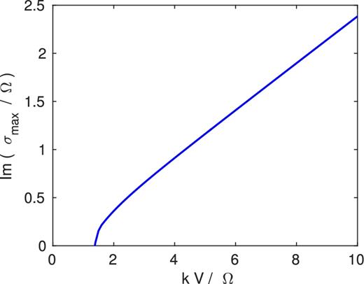
Parasitic growth rates maximized over K_η for different VSI amplitudes (i.e. Rossby numbers) kV/Ω. Here q = −0.01 and the underlying VSI mode possesses sinusoidal structure, f(ξ) = sin ξ. Because V increases with time (at the slow rate |q|Ω) the x-axis may be thought of as a proxy for time.

Open in new tab Download slide

3.2 Non-axisymmetric instability

We next consider non-axisymmetric parasitic instabilities. Because of their transient growth, such parasites may only be important when the VSI achieves large amplitudes, but when in this regime they should dominate because they can more effectively extract shear energy than their axisymmetric counterparts. They are also of interest because they are clearly the means by which axisymmetry breaks down in the VSI dynamics. The vortices they produce will be better aligned with the disc plane, unlike those that originate from the axisymmetric parasites discussed in the previous subsection.

After writing down the linearized equations, we adopt the same approximation schemes as in Sections 3.1.2 and 3.1.3 with the aim of deriving equations analogous to (34) and (39). Assuming the y dependence of modes is such that

\begin{equation*} \boldsymbol {u}_2,{\, }P_2 \propto {\rm exp}({\rm i}K_y y), \end{equation*}

where K_y is the azimuthal wavenumber, we obtain the perturbation equations

\begin{eqnarray} {\rm i}\overline{\sigma } u_{2\zeta } = -\mathrm{\partial} _\zeta h_2 + \frac{2\Omega k_x}{k} u_{2y}, \end{eqnarray}

(40)

\begin{eqnarray} {\rm i}\overline{\sigma } u_{2y} = -{\rm i}K_y h_2 - (V\bar{u}_{1y}\mathrm{\partial} _\zeta f){\, }u_{2\zeta } - \frac{1}{2}\Omega u_{2x} + q\Omega u_{2z}, \end{eqnarray}

(41)

\begin{eqnarray} {\rm i}\overline{\sigma } u_{2\eta } = - (V\bar{u}_{1\eta }\mathrm{\partial} _\zeta f){\, }u_{2\zeta }- \mathrm{\partial} _\eta h_2 -\frac{2\Omega k_z}{k} u_{2y}, \end{eqnarray}

(42)

\begin{eqnarray} 0= \mathrm{\partial} _\zeta u_{2\zeta } + \mathrm{\partial} _\eta u_{2\eta } + {\rm i}K_y u_{2y}, \end{eqnarray}

(43)

where h₂ = P₂/ρ₀, as before, and

\begin{equation*} \overline{\sigma }=-{\rm i}\mathrm{\partial} _t -K_y(3x/2+ qz)\Omega + V(\boldsymbol {K}\cdot \bar{\boldsymbol {u}}_1){\, }f(\xi ), \end{equation*}

with |$\boldsymbol {K}= K_y\boldsymbol {e}_{y}- {\rm i} \boldsymbol{e}_{\eta} \partial_{\eta} $|⁠. We remark that in the new coordinates

\begin{equation*} \frac{3}{2}x+qz=\left(\frac{3}{2}k_x+qk_z \right)\zeta /k+\left(qk_x-\frac{3}{2}k_z \right)\eta /k. \end{equation*}

On account of its explicit dependence on ζ, η, and t, the above system is not strictly separable. But if we employ the small |q| limit as in Section 3.1.2, some separability may be restored. The fastest growing VSI modes possess k_z = O(qk_x), and so

\begin{equation*} \frac{3}{2}x+qz=\frac{3}{2}\zeta +{\rm O}(q\eta ). \end{equation*}

Thus in the limit |q| → 0, the system becomes separable in η and t as well as y so that we may assume that

\begin{equation*} \boldsymbol {u}_2,{\, }P_2 \propto {\rm exp}({\rm i}(\sigma t+ K_yy+K_\eta \eta ). \end{equation*}

Then

\begin{equation} \overline{\sigma }\rightarrow \sigma - \frac{3}{2}K_y\zeta \Omega + V(\boldsymbol {K}\cdot \bar{\boldsymbol {u}}){\, }f(\xi ), \end{equation}

(44)

and |$\boldsymbol {K} \rightarrow K_y\boldsymbol {e}_{y}+ K_\eta \boldsymbol {e}_\eta .$| A second-order ODE may now be derived which we consider in two limits.

3.2.1 Tight-winding limit

The first limit we treat is the tight-winding approximation for which the Keplerian shear may be neglected. From (44) this requires |$K_y\Omega /k \ll |{\boldsymbol K} V|.$| Assuming, as above, that |$|{\boldsymbol K}|/k\sim 1,$| this corresponds to |$K_y/K_\eta \ll |{\boldsymbol K}V |/\Omega .$| Thus in the limit of sufficiently small K_y/K_η, the Keplerian shear may be neglected. In this limit the set of equations (40)–(43) becomes equivalent to the set (24)–(27) that governs the axisymmetric problem. Accordingly, equation (34) is recovered in the small q, small K_y/K_η limit.

3.2.2 The large VSI-amplitude limit

In this limit one assumes, in addition to small |q|, that |kV|/Ω ≫ 1, but there is no requirement that K_y be small. In this case all the terms explicitly proportional to Ω in equations (40)–(43) can be dropped. The system reduces to a single second-order ODE

\begin{equation} \frac{{\rm d}^2 u_{2\zeta }}{{\rm d}\zeta ^2} -\left(K^2 + \frac{ V(\boldsymbol {K}\cdot \bar{\boldsymbol {u}})({\rm d}^2f/{\rm d}\zeta ^2)}{\sigma + V(\boldsymbol {K}\cdot \bar{\boldsymbol {u}}){\, }f(\xi )}\right) u_{2\zeta } = 0. \end{equation}

(45)

This is again a form of Rayleigh's equation and the discussion in Section 3.1.3 regarding (39) applies here also. Note that the non-axisymmetric growth rates will be larger than the corresponding axisymmetric growth rates in this limit by a factor |$K/(K_\eta \overline{u}_\eta ) \approx 2$|⁠. This is because the non-axisymmetric wavevector is free to be parallel to the direction of the shear flow.

3.3 Discussion

Putting together these theoretical details, we can construct a relatively straightforward account of a VSI mode's growth and evolution.

First, the VSI will grow relatively unhindered up to ‘moderate’ amplitudes, 0 < V < Ω/k. It is a non-linear solution, so there are no non-linear effects to intervene. During this time, non-axisymmetric parasitic modes will fail to get any traction because they only grow transiently over a shear time 1/Ω: if their growth rates during this time are (at most) proportional to kV then they will only amplify by a factor exp[(Vk/Ω)(e − 1)] ≲ 5.575, most likely insufficient to overtake their host. Axisymmetric parasites are untroubled by the shear; however, they are strongly stabilized by the disc's rotation when at these low Rossby numbers (as explained in Section 3.1.2 and illustrated in Fig. 4). Only when the VSI amplitude is above a critical value V > V_crit ≳ Ω/k will axisymmetric parasites grow exponentially and ultimately disturb the underlying mode. Near the same point non-axisymmetric parasites may also achieve greater amplitudes during their windows of growth. This will all occur at some second critical value V = V_max. It is unclear whether the axisymmetric or non-axisymmetric parasites will launch the first successful attack. It is possible that they may emerge concurrently.

3.3.1 Maximum VSI amplitudes

The precise value of V_crit is determined by the details of the flow, in particular by the form of f(ξ). The value of the maximum VSI amplitude V_max is the amplitude at which the VSI mode is significantly disrupted. It is necessarily larger than V_crit, and may be estimated using arguments presented in Latter (2016).

Suppose the VSI grows according to the equation V(t) = V_crit exp(|q|Ωt), so that at t = 0 the VSI has hit the first critical amplitude. Suppose from that point the parasite amplitude p grows according to dp/dt = kV(t)p(t), with p = p₀ at t = 0. The latter ODE can be solved and the time at which the parasite amplitude equals its host (p = V) calculated, an event that occurs when the VSI attains the amplitude:

\begin{eqnarray} V = V_{\rm max} = -\frac{q\Omega }{k}W_{-1}\left[-\frac{kp_0}{q\Omega }{\rm exp}\left(\frac{-k V_{\rm crit}}{q\Omega }\right)\right] \end{eqnarray}

(46)

\begin{eqnarray} \gtrsim V_{\rm crit}\left[1+ |q|\ln \left(\frac{|q|}{kp_0/\Omega }\right) \right], \end{eqnarray}

(47)

where W₋₁ is the second branch of Lambert's function, and the final estimate comes from its asymptotic expansion in small argument and by setting V_crit ≳ Ω/k (see Corless et al. 1996; Latter 2016). The second term in the square brackets depends on the relative sizes of |q| and the noise from which the parasite grows. Even if this ratio is large, it will be the moderated by the log and the q pre-factor, so for simplicity we set V_max ≳ V_crit ≳ Ω/k. In summary, we do not expect these three velocity scales to differ by very much.

In order to develop the theory further and make concrete estimates, we need to know what value k takes, i.e. the characteristic wavenumber of the fastest growing VSI mode, which means invoking physics so far neglected. Consider a disc region in which the diffusion approximation holds (at 1 au, say, in the low-mass disc model of Lesur and Latter 2016). From Section 2.4 and Fig. 3, we observe that the fastest growing VSI modes possess |$k>\sqrt{\Omega /\kappa }$|⁠. An upper bound on V_max is hence

\begin{equation*} V_{\rm max}\sim \sqrt{\kappa \Omega }\sim {\rm Pe}^{-1/2}c_{\rm s}, \end{equation*}

where c_s is the sound speed and Pe is the Peclet number, as earlier. At 1 au in our model Pe ∼ 10³, and so the characteristic VSI amplitudes are a few per cent of the disc sound speed. More massive disc models may give a similar estimate out to radii as far as 10 au. In our low-mass model, however, larger radii are only marginally within the compass of the local approximation, or are outside the diffusion approximation. Nonetheless, the estimated velocity amplitudes might increase to some 10 per cent of the local sound speed, and hence should be significant.

An alternative, and more general, upper limit on V can be obtained by noting that k ∼ k_x ∼ |1/q|k_z ≳ |1/qH|, where H is the disc scale height. VSI modes with k_z ∼ 1/H might correspond to the ‘body modes’ witnessed in global simulations and vertically stratified boxes (Nelson, Gressel & Umurhan 2013; Barker and Latter 2015). This then implies that V_max ≲ |q|c_s ∼ (H/R)c_s. Once again, we find that the maximum turbulent speeds should be a few per cent to 10 per cent the local sound speed.

3.3.2 Saturation and comparison with simulations

These maximum amplitudes we expect to be attained at the beginning of the VSI evolution. But what happens next, after the system breaks down into a turbulent state and saturates? What velocity amplitudes might we expect in this state? The answers to these questions lie in the radiative driving of the vertical shear and its relative strength in comparison with the VSI. One can envisage two limits.

First, suppose that the vertical shear is strictly enforced by the star's radiation field, and so the VSI is relatively ineffective in smoothing it out. This is certainly the scenario in our shearing box model, in which the vertical shear is ‘hard-wired’ into the box. It is also the case for isothermal global simulations or ideal gas simulations with short relaxation times (Nelson, Gressel & Umurhan 2013). The VSI will churn away upon the vertical shear, but be unable to erase it. One might then be tempted to ascribe the general VSI saturation to the parasitic modes, rather than a weakening of the underlying unstable state. The parasites limit VSI growth via a transfer of energy to smaller scales and ultimately the viscous length, and will set their characteristic amplitude. This turbulent amplitude would then be ≲ V_max, a few per cent or more of the sound speed, and indeed this is in rough agreement with global simulations (Nelson, Gressel & Umurhan 2013; Stoll and Kley 2014). In fact, the relatively large amplitudes produced by these simulations, and the fact that the saturated state is characterized by non-linear structures similar in form to linear modes, provides strong evidence in favour of this interpretation. Large amplitudes come about because (a) the linear modes are non-linear solutions and (b) parasitic modes that might limit them are hampered by the stabilizing effect of rotation.

Parasitic modes in this context may not only limit the amplitudes of the VSI but also direct energy from them into the formation of non-axisymmetric structures, such as vortices. Being essentially Kelvin–Helmholtz in nature, the ‘wrapping up’ of the VSI vortex layers is a natural outcome of their evolution. As shown in Richard, Nelson & Umurhan (2016), vortex formation is key to the breakdown of axisymmetry in the VSI saturation, and hence to the possibility of any accretion. We observe that the vortices formed in our local model are not oriented flush with the orbital plane, but are aligned with the VSI flow |$\bar{\boldsymbol {u}}$|⁠. Consequently, they are tilted upward or downward relative to the orbital plane by an angle ≈60°, and will not appear columnar as in the subcritical baroclinic instability or ‘Rossby wave’ instability (Lovelace et al. 1999; Lesur and Papaloizou 2010). Indeed, Richard, Nelson & Umurhan (2016) find that the vortex structures possess both radial and vertical variations, on some length of order 0.1H. According to our analysis this wavelength should correspond to that of the fastest growing parasites, which in turn will approximate the radial wavelength of the underlying VSI modes. This is also in keeping with the global simulations.

The second limit corresponds to a scenario in which the baroclinic driving is very weak and the VSI overpowers the vertical shear, effectively smoothing it out. Initially the VSI might achieve large amplitudes but, as the destabilizing gradient (the vertical shear) is destroyed, it will settle down into a low-amplitude sluggish state near marginal stability (as in certain simulations in Stoll and Kley 2014). In this case the saturated amplitude will be ≪V_max. Any vortices, or other non-axisymmetric structure, created in the initial burst will ultimately die and axisymmetry will be restored. Consequently, no accretion is to be expected.

In reality, most discs at a given time will lie somewhere in between these two extremes. Detailed modelling of the baroclinic driving and a sequence of careful and detailed global simulations are needed to determine the expected range of states the VSI occupies. It should be stressed that in order to sustain vortex production (and accretion) the VSI must be permitted to achieve large amplitudes. If it is too efficient, then it will settle down into a less interesting low state.

4 VERTICAL SHEAR AND MAGNETIC FIELDS

In certain regions of a PP disc magnetic fields may have some influence, even in dead zones where the MRI is suppressed. Certainly in their upper layers, which are subject to significant photoionization, the gas may couple effectively to a mean magnetic field, which in turn may be too strong to permit the MRI but rather a magnetocentrifugal wind (Bai and Stone 2013; Bai 2014; Lesur, Kunz & Fromang 2014). We may then ask what effect does magnetism have on the onset of the VSI? Conversely, MRI-active regions may exhibit vertical shear: how would that impact on the MRI?

In this section we make a start on these questions by determining the linear response of ionized fluid pierced by a mean magnetic field. Non-ideal effects are only dealt with in passing, and could form the basis of future work.

4.1 Governing equations and magnetic equilibria

The equations governing our ionized local slab of disc are now

\begin{eqnarray} \mathrm{\partial} _t\boldsymbol {u}+ \boldsymbol {u}\cdot \nabla \boldsymbol {u}= &-&\frac{1}{\rho }\nabla P_{\rm tot} -2\Omega \boldsymbol {e}_{z}\times \boldsymbol {u}\nonumber \\ &-&\,\Omega (3x +2z q) \boldsymbol {e}_{x}+\frac{\boldsymbol {B}\cdot \nabla \boldsymbol {B}}{4\pi \rho }, \end{eqnarray}

(48)

\begin{eqnarray} \mathrm{\partial} _t\boldsymbol {B}+ \boldsymbol {u}\cdot \nabla \boldsymbol {B}&= \boldsymbol {B}\cdot \nabla \boldsymbol {u}, \end{eqnarray}

(49)

alongside |$\nabla \cdot \boldsymbol {u}=\nabla \cdot \boldsymbol {B}=0$|⁠, where |$\boldsymbol {B}$| is the magnetic field, and P_tot denotes the sum of gas and magnetic pressures.

This system admits the following equilibrium, similar to before

\begin{equation*} \boldsymbol {u}=\boldsymbol {u}_0=-\frac{1}{2}(3x+2qz)\boldsymbol {e}_{y},\quad P_{\rm tot}=P_0,\quad \boldsymbol {B}=\boldsymbol {B}_0, \end{equation*}

where P₀ is a constant scalar and |$\boldsymbol {B}_0$| is a constant vector. We are completely free to specify the y component of |$\boldsymbol {B}_0$| but the radial and vertical components are constrained by Ferraro's law, i.e. the y component of the induction equation |$\boldsymbol {B}_0\cdot \nabla \boldsymbol {u}_0=0$|⁠. This states that in order to have a steady equilibrium we must have

\begin{equation} B_{0x}= -\frac{2q}{3} B_{0z}. \end{equation}

(50)

In other words, the B_y generated by the radial shear (working on B_x) must be exactly balanced by the B_y created by the vertical shear (working on B_z). This is a key issue in constructing magnetic equilibria in the presence of vertical shear: both vertical and radial magnetic fields must be present in the correct amounts. (This issue was overlooked in Urpin and Brandenburg 1998.) Global examples of such fields have been computed by Ogilvie (1997), and vertically stratified examples by Riols et al. (2016) (see also Papaloizou & Szuszkiewicz 1992). Typically the poloidal field varies with space but in our simple local incompressible model the magnetic field is conveniently constant. Finally, for simplicity, we set the y component of |$\boldsymbol {B}$| to zero.

4.2 Perturbations and the dispersion relation

To understand the two instabilities in question we perturb the equilibrium described above by disturbances |$\boldsymbol {u}^{\prime }$|⁠, |$P_{\rm tot}^{\prime },$| and |$\boldsymbol {B}^{\prime }$|⁠. Assuming that they are ∝ exp(ik_xx + ik_zz + st), the linearized equations governing their evolution may be written as

\begin{eqnarray} s u_x^{\prime } = -{\rm i}k_x h^{\prime } + 2\Omega u_y^{\prime } + {\rm i} (\boldsymbol {v}_{\rm A}\cdot \boldsymbol {k}) b_x^{\prime }, \end{eqnarray}

(51)

\begin{eqnarray} s u_y^{\prime } = -\frac{1}{2}\Omega u_x^{\prime } + \Omega q u_z^{\prime } + {\rm i} (\boldsymbol {v}_{\rm A}\cdot \boldsymbol {k}) b_y^{\prime }, \end{eqnarray}

(52)

\begin{eqnarray} s u_z^{\prime } = -{\rm i}k_z h^{\prime } + {\rm i} (\boldsymbol {v}_{\rm A}\cdot \boldsymbol {k}) b_z^{\prime }, \end{eqnarray}

(53)

\begin{eqnarray} s b_x^{\prime } = {\rm i}(\boldsymbol {v}_{\rm A}\cdot \boldsymbol {k}) u_x^{\prime }, \end{eqnarray}

(54)

\begin{eqnarray} s b_y^{\prime } = {\rm i} (\boldsymbol {v}_{\rm A}\cdot \boldsymbol {k}) u_y^{\prime } - \frac{3}{2}\Omega b_x^{\prime } - q\Omega b_z^{\prime }, \end{eqnarray}

(55)

\begin{eqnarray} s b_z^{\prime } = {\rm i}(\boldsymbol {v}_{\rm A}\cdot \boldsymbol {k}) u_z^{\prime }, \end{eqnarray}

(56)

\begin{eqnarray} 0= {\rm i}k_x u_x^{\prime } + {\rm i}k_z u_z^{\prime }, \end{eqnarray}

(57)

where |$h^{\prime }= P_{\rm tot}^{\prime }/\rho$| with the perturbed and background Alfvén velocities |$\boldsymbol {b}^{\prime }=\boldsymbol {B}^{\prime }/\sqrt{4\pi \rho }$| and |$\boldsymbol {v}_{\rm A}=\boldsymbol {B}_0/\sqrt{4\pi \rho }$|⁠, respectively, and |$\boldsymbol {k}=\boldsymbol {e}_{x}k_x+ \boldsymbol {e}_{z}k_z$|⁠. On account of the incompressibility condition the solution automatically satisfies |$\nabla \cdot \boldsymbol {B}^{\prime }=0.$| This means that it satisfies the non-linear equations as well as the linear ones. But note that when k_x = 0, incompressibility enforces |$u_z^{\prime }=0$| and consequently |$b^{\prime }_z=h^{\prime }=0$|⁠. In that case terms involving q disappear, and the resulting MRI ‘channel flows’ do not feel the vertical shear whatsoever.

After some algebra these equations can be reduced to a biquadratic dispersion relation for the growth rate s:

\begin{eqnarray} s^4 &+& \left[ 2(\boldsymbol {v}_{\rm A}\cdot \boldsymbol {k})^2+\epsilon ^2\Omega ^2 +2\epsilon ^2\Omega ^2q \frac{k_x}{k_z} \right]s^2 \nonumber \\ &+& \, (\boldsymbol {v}_{\rm A}\cdot \boldsymbol {k})^2\left[ (\boldsymbol {v}_{\rm A}\cdot \boldsymbol {k})^2 -3\Omega ^2\epsilon ^2 + 2\epsilon ^2\Omega ^2q \frac{k_x}{k_z} \right]=0, \end{eqnarray}

(58)

in which we have introduced the additional notation

\begin{equation*} \epsilon \equiv \frac{k_z}{k}=\left(1+\frac{k_x^2}{k_z^2}\right)^{-1/2}, \end{equation*}

as in Latter, Fromang & Faure (2015).

We can obtain stability criteria by first noting that the two roots for s² obtained from (58) are always real. Instability occurs when one of these is positive, which happens when either (a) the coefficient of s² is negative or (b) when this coefficient is positive but the last term in the dispersion relation is negative. When there is no background magnetic field (⁠|$\boldsymbol {v}_{\rm A}=\mathbf {0}$|⁠), the condition (a) reduces to the hydrodynamical VSI instability criterion, equation (14), which states that q(k_x/k_z) < −1/2. The presence of a non-zero magnetic field (⁠|$\boldsymbol {v}_{\rm A}\ne \mathbf {0}$|⁠), no matter how small, changes the picture abruptly. Then the condition (b) is the easiest of the two to satisfy, yielding

\begin{equation} (\boldsymbol {v}_{\rm A}\cdot \boldsymbol {k})^2 < \frac{k_z^2}{k^2}\Omega ^2 \left(3 - 2q\frac{k_x}{k_z}\right), \end{equation}

(59)

that is, when the Alfvèn frequency is less than the characteristic frequency defined by the right-hand side. This criterion captures both the MRI and the VSI.

4.3 The MRI and vertical shear

We first examine how the MRI is altered by vertical shear. When q = 0, we reproduce the well-known results for the purely vertical field MRI, |$\boldsymbol {B}_0\propto \boldsymbol {e}_{z}$|⁠. The fastest growing modes are channel modes, while ‘radial modes’, with k_x ≠ 0, grow a factor ε slower. As explained in Latter, Fromang & Faure (2015), radial modes exhibit vertical circulation that impedes the MRI instability mechanism. An alternative way to think about this is in terms of the competition between the effects of rotation and magnetism: when k_x = 0 the characteristic rate of destabilization, on account of the rotation profile, is ∝ Ω, but when k_x ≠ 0 it is ∝ εΩ < Ω. The stabilizing influence of magnetic tension is accordingly more effective for a given Alfvèn frequency |$(\boldsymbol {v}_{\rm A}\cdot \boldsymbol {k})$|⁠. As a consequence of this, we expect the MRI branch of modes to be most important (and the most characteristic) for wavenumbers oriented nearly vertically, i.e. when k_x ≪ k_z, which is in convenient contrast to the VSI, for which the opposite limit pertains.

We find the expression for the squared growth rate, solving equation (58) under the assumption that criterion (b) applies, equation (59). We next consider it as a function of |$(\boldsymbol {v}_{\rm A}\cdot \boldsymbol {k})^2$|⁠, and find its maximum value. This occurs when

\begin{equation} (\boldsymbol {v}_{\rm A}\cdot \boldsymbol {k})^2= \frac{15}{16}\epsilon ^2\Omega ^2 -\frac{1}{4}q\frac{k_x}{k_z}\epsilon ^2\Omega ^2\left(1 + q\frac{k_x}{k_z}\right), \end{equation}

(60)

the first term on the right should be familiar from previous studies of the MRI, while the second comes from the vertical shear. Substituting this expression into the growth rate obtained from (58), we obtain a remarkably simple expression for the maximum rate:

\begin{equation} s_{\rm max}= \frac{3}{4}\epsilon \Omega \left(1-\frac{2}{3}\frac{k_x}{k_z}q\right). \end{equation}

(61)

It corresponds to the classical expression for maximum growth rate for the MRI (e.g. Latter, Fromang & Faure 2015) with a ‘correction’ proportional to q that comes from the vertical shear. The bracketed expression in equation (61) is, in fact, proportional to |$(\boldsymbol {k}\times (\nabla \Omega ))\cdot \boldsymbol {e}_y$|⁠, and so complete stabilization occurs for modes with |$\boldsymbol {k}$| parallel to the angular velocity gradient. The components of the wavenumber then satisfy k_x/k_z = 2/(3q).

Furthermore, we may maximize (61) with respect to k_x/k_z, and find that |$s_{\rm max}= (3/4)\Omega + (5/81)q^2\Omega +\mathcal {O}(q^4)$|⁠, assuming small q, and this occurs when k_x/k_z ≈ −(1/9)q. Essentially this is a channel mode, but the slightly elevated growth rate indicates that the MRI can draw some energy from the background vertical shear in addition to the radial shear, thus acting partly like the VSI. Overall, however, the fastest growing and most important MRI modes, for which k_z > k_x, are not especially impacted by the vertical shear, if indeed we expect q ≪ 1.

4.4 The VSI and magnetic fields

The VSI lies on the same branch of the dispersion relation as the MRI, and so it is not easy to distinguish the two: as k_x/k_z goes from very small to very large values the MRI smoothly morphs into the VSI. To illustrate this point we plot in Fig. 5 growth rate contours in the |$[(\boldsymbol {v}_{\rm A}\cdot \boldsymbol {k})/\Omega _0,{\, } k_x/k_z]$| plane for q = 0 and q = −0.3. In the latter case we observe low growth for large k_x/k_z and small |$(\boldsymbol {v}_{\rm A}\cdot \boldsymbol {k})/\Omega _0$|⁠, which we associate with the VSI, and large growth for small k_x/k_z and |$(\boldsymbol {v}_{\rm A}\cdot \boldsymbol {k})/\Omega _0\sim 1$|⁠, which we associate with the MRI.

$Top panel: coloured contours of the MRI growth rate when q = 0 in the $[(\boldsymbol {v}_{\rm A}\cdot \boldsymbol {k})/\Omega _0,{\, } k_x/k_z]$ plane. Note the symmetry about the horizontal axis. Bottom panel: contours of the MRI and VSI growth rates when q = −0.3. Observe the marked asymmetry about the horizontal axis, and the extension of growth to large kx/kz.$

Figure 5.

Top panel: coloured contours of the MRI growth rate when q = 0 in the |$[(\boldsymbol {v}_{\rm A}\cdot \boldsymbol {k})/\Omega _0,{\, } k_x/k_z]$| plane. Note the symmetry about the horizontal axis. Bottom panel: contours of the MRI and VSI growth rates when q = −0.3. Observe the marked asymmetry about the horizontal axis, and the extension of growth to large k_x/k_z.

Open in new tab Download slide

To disentangle the VSI algebraically, we let k_x/k_z = −1/q, the wavevector orientation that yields maximum VSI growth in the absence of a magnetic field. Both expressions (60) and (61) should hold for such a mode. Plugging in our value for k_x/k_z we find that maximum growth occurs at very small values of |$(\boldsymbol {v}_{\rm A}\cdot \boldsymbol {k})^2\sim q^2$|⁠, but with maximum growth s_max = (5/4)qΩ, slightly larger than in the hydrodynamical case. This indicates that for exceedingly light magnetic tension, the VSI is slightly amplified.

Overall, however, the impact of magnetic tension is stabilizing, with stability occurring when (59) is violated. For VSI wavevector orientations k_x/k_z ∼ −1/q, the criterion can be reframed in terms of the vertical component of the magnetic tension. Unless v_Azk_z is very small, the mode is suppressed:

\begin{equation} v_{{\rm A}z}k_z \lesssim q\Omega . \end{equation}

(62)

Put another way, for a given v_Az, the critical vertical wavelength for instability is long, so as to best escape the stabilizing magnetic tension.

But in order for the VSI modes to even fit into the disc these lengthscales must be less than H. This furnishes us with an instability criterion. We find that the VSI can only occur in magnetized discs if

\begin{equation} \beta \gtrsim q^{-2}, \end{equation}

(63)

where β is the average plasma beta within |Z| < H (the MRI only requires that β ≳ 1). Using the estimate q ∼ H/R ∼ 0.05 the criterion becomes β ≳ 400. Note that the critical β may be significantly larger for smaller scale VSI modes, such as those that typically appear in the surface layers of the disc, and furthermore the local β in these layers may be low indeed.

4.5 Ohmic diffusion

In the dead zones of PP discs, magnetic diffusion will alter the results of the previous sections. In particular, it will weaken magnetic tension and the VSI will find it easier to grow. We now estimate how much diffusion is needed to ‘rescue’ the VSI.

By comparing frequencies, magnetic diffusion dominates tension when ηk² ≳ v_Ak, where η is Ohmic resistivity. For fixed v_A, this means that on scales k ≳ k_D ≡ v_A/η magnetic tension may be overcome and hence neglected. On the other hand, the VSI is suppressed when its growth rate ∼qΩ is equal or less the Alfvén frequency v_Ak. This occurs on wavenumbers k ≳ k_S ≡ qΩ/v_A. Putting these two estimates together, we recognize that the VSI is impeded when k_S ≲ k ≲ k_D, and unimpeded for other wavenumbers. In fact, magnetic tension is completely subdued by diffusion for all modes when k_D ≲ k_S which gives the condition

\begin{equation} E_\eta \lesssim q, \end{equation}

(64)

where the Ohmic Elsasser number is defined to be |$E_\eta = v_{\rm A}^2/(\Omega \eta )$|⁠. Note that violation of equation (64) does not mean the VSI fails to appear: unstable VSI modes will still operate on sufficiently short (and possibly sufficiently long) scales.

To estimate E_η requires knowledge of the strength of the background vertical field. For a mid-plane β = 10⁵, Lesur, Kunz & Fromang (2014), using the minimum-mass solar nebula, estimate that E_η < 10⁻⁴ when |z| < H at R = 1 au, and E_η = 0.1 − 1 when R = 10 au. Given that q ∼ H/R ∼ 0.05, we recognize that at 1 au the VSI is free of magnetic tension; but further out in the disc it may be worth considering the role of magnetic fields a little more closely, especially when those fields are strong.

5 CONCLUSION

In this paper we have established a number of theoretical results pertaining to the onset and saturation of the VSI in PP discs. Using the Boussinesq approximation, we show that the linear VSI modes are non-linear solutions whose spatial structure need not be limited to sinusoids. Being double-diffusive, the instability grows at its maximum rate ∼(H/R)Ω on a range of wavelengths bracketed from below by (H/R)^−1/2Re^−1/2H and above by (H/R)^1/2Pe^−1/2H, where Re and Pe are the Reynolds and Peclet numbers. On sufficiently short scales and in certain disc regions the diffusive approximation breaks down and these estimates require moderate revision. In this case, maximum growth is assured if the gas's cooling rate is much greater than (R/H)Ω (in agreement with Lin and Youdin 2015). We apply these estimates to a low-mass disc and demonstrate that the VSI is prevalent from 1 au outward, moving from shorter to longer scales with disc radius.

The VSI modes cannot grow indefinitely, as they are subject to parasitic instabilities of Kelvin–Helmholtz type. The onset of the parasites, however, is significantly delayed: axisymmetric instability is impeded by the gas's stabilizing radial angular momentum gradient, whereas non-axisymmetric instability is foiled by the disc's shear. As a consequence, the VSI achieves relatively large amplitudes before breaking down, these characterized by Rossby numbers greater than 1 and fluid velocities a few per cent or more of the sound speed. This makes a striking contrast to the convective overstability, whose amplitudes are kept generally low by parasites (Latter 2016). The delay in VSI disruption might explain some features witnessed in global simulations, such as the dominance of large amplitude linear waves, at least initially (Nelson, Gressel & Umurhan 2013). We note that our analysis strictly holds only for non-linear modes that remain shortscale, and that the body modes are not represented in a Boussinesq model. Nonetheless, the physical effects outlined above will also work on larger scales and should get in the way of their disruption as well.

The parasites may play an influential part in the VSI's subsequent saturation. If the background vertical shear is forcibly maintained by stellar irradiation, the parasites may set the amplitude of the resulting quasi-steady turbulent state. If, however, the VSI is efficient in erasing the vertical shear, they may be less important. Significantly, parasitic instabilities are the route by which the VSI's axisymmetry is broken; the subsequent turbulence may then transport angular momentum. In so doing they create vortices, not perfectly aligned with the disc plane. Vortex production is a robust process, and VSI modes on all scales can generate them. As discussed at length elsewhere, vortices can accumulate solid particles, though in this context it may be complicated by their non-trivial vertical structure. Their geometry and limited lifetime are other variables deserving of further study (Richard, Nelson & Umurhan 2016).

Finally we include magnetic fields in the analysis. Because of the vertical shear it is important to be careful to set up a meaningful time-independent magnetic equilibrium. We find that the MRI is not impacted greatly by the vertical shear, and the fastest growing modes (channel modes) are not affected at all. In contrast, the VSI is completely suppressed by magnetic tension, for (average) plasma betas below ≳ q⁻² ∼ (R/H)². Ohmic diffusion can rescue the VSI, however, if the local Elsasser number is less than q ∼ H/R.

Acknowledgements

The authors would like to thank Andrew Youdin, Adrian Barker, and the anonymous referee for useful comments that helped improve the manuscript. We also thank Tobias Heinemann for a close reading of an earlier draft. This work is partially funded through STFC grant ST/L000636/1.

REFERENCES

Bai

X.-N.

,

2014

,

ApJ

,

791

,

137

Crossref

Search ADS

Balbus

S. A.

,

Hawley

J. F.

,

2006

,

ApJ

,

652

,

1020

Crossref

Search ADS

Balbus

S. A.

,

Schaan

E.

,

2012

,

MNRAS

,

426

,

1546

Crossref

Search ADS

Balbus

S. A.

,

Bonart

J.

,

Latter

H. N.

,

Weiss

N. O.

,

2009

,

MNRAS

,

400

,

176

Crossref

Search ADS

Barker

A. J.

,

Latter

H. N.

,

2015

,

MNRAS

,

450

,

21

Crossref

Search ADS

Booker

J. P.

,

Bretherton

F. P.

,

1967

,

JFM

,

27

,

513

Crossref

Search ADS

Boyd

J. P.

,

2001

,

Chebyshev and Fourier Spectral Methods

, 2nd edn.

Dover Press

,

New York

Google Scholar

Google Preview

OpenURL Placeholder Text

WorldCat

Caleo

A.

,

Balbus

S. A.

,

2016

,

MNRAS

,

457

,

1711

Crossref

Search ADS

Caleo

A.

,

Balbus

S. A.

,

Tognelli

E.

,

2016

,

MNRAS

,

460

,

338

Crossref

Search ADS

Corless

R. M.

,

Gonnet

G. H.

,

Hare

D. E. G.

,

Jeffrey

D. J.

,

Knuth

D. E.

,

1996

Adv. Comp. Math.

,

5

,

329

Crossref

Search ADS

Drazin

P. G.

,

Reid

W. H.

,

1981

,

Hydrodynamic Stability

.

Cambridge Univ. Press

,

Cambridge

Google Scholar

Google Preview

OpenURL Placeholder Text

WorldCat

Fricke

K.

,

1968

,

Z. Astrophys.

,

68

,

317

Fromang

S.

,

Lesur

G.

,

2017

,

preprint (arXiv:1705.03319)

Goldreich

P.

,

Schubert

G.

,

1967

,

ApJ

,

150

,

571

Crossref

Search ADS

Goodman

J.

,

Xu

G.

,

1994

,

ApJ

,

432

,

213

Crossref

Search ADS

James

H. A.

,

Kahn

F. D.

,

1970

,

A&A

,

5

,

232

James

H. A.

,

Kahn

F. D.

,

1971

,

A&A

,

12

,

332

Johnson

B. M.

,

Gammie

C. F.

,

2005

,

ApJ

,

626

,

978

Crossref

Search ADS

Knobloch

E.

,

Spruit

H. C.

,

1982

,

A&A

,

113

,

261

Latter

H. N.

,

2016

,

MNRAS

,

455

,

2608

Crossref

Search ADS

Latter

H. N.

,

Balbus

S. A.

,

2009

,

MNRAS

,

399

,

1048

Crossref

Search ADS

Latter

H. N.

,

Papaloizou

J. C. B.

,

2017

,

MNRAS

,

472

,

1432

Crossref

Search ADS

Latter

H. N.

,

Lesaffre

P.

,

Balbus

S. A.

,

2009

,

MNRAS

,

394

,

715

Crossref

Search ADS

Latter

H. N.

,

Fromang

S.

,

Faure

J.

,

2015

,

MNRAS

,

453

,

3257

Crossref

Search ADS

Lesur

G.

,

Latter

H. N.

,

2016

,

MNRAS

,

462

,

4549

Crossref

Search ADS

Lesur

G.

,

Papaloizou

J. C. B.

,

2010

,

A&A

,

513

,

60

Crossref

Search ADS

Lesur

G.

,

Kunz

M. W.

,

Fromang

S.

,

2014

,

A&A

,

566

,

A56

Crossref

Search ADS

Li

L.-X.

,

Goodman

J.

,

Narayan

R.

,

2003

,

ApJ

,

593

,

980

Crossref

Search ADS

Lin

M.-K.

,

Youdin

A. N.

,

2015

,

ApJ

,

811

,

17

Crossref

Search ADS

Lovelace

R. V. E.

,

Li

H.

,

Colgate

S. A.

,

Nelson

A. F.

,

1999

,

ApJ

,

513

,

805

Crossref

Search ADS

Malygin

M. G.

,

Klahr

H.

,

Semenov

D

,

Henning

T.

,

Dullemond

C. P.

,

2017

,

A&A

,

605

,

A30

Crossref

Search ADS

McNally

C. P.

,

Pessah

M. E.

,

2015

,

ApJ

,

811

,

121

Crossref

Search ADS

Nelson

R. P.

,

Gressel

O.

,

Umurhan

O. M.

,

2013

,

MNRAS

,

435

,

2610

Crossref

Search ADS

Ogilvie

G. I.

,

1997

,

MNRAS

,

288

,

63

Crossref

Search ADS

Papaloizou

J.

,

Szuszkiewicz

E.

,

1992

,

Geophys. Astrophys. Fluid Dyn.

,

66

,

223

Crossref

Search ADS

Pessah

M. E.

,

Goodman

J.

,

2009

,

ApJ

,

698

,

72

Crossref

Search ADS

Richard

S.

,

Nelson

R. P.

,

Umurhan

O. M.

,

2016

,

MNRAS

,

456

,

3571

Crossref

Search ADS

Riols

A.

,

Ogilvie

G. I.

,

Latter

H. N.

,

Ross

J. P.

,

2016

,

MNRAS

,

463

,

3096

Crossref

Search ADS

Simon

J. B.

,

Lesur

G.

,

Kunz

M. W.

,

Armitage

P. J.

,

2015

,

MNRAS

,

454

,

1117

Crossref

Search ADS

Stoll

M. H. R.

,

Kley

W.

,

2014

,

A&A

,

572

,

A77

Crossref

Search ADS

Stoll

M. H. R.

,

Kley

W.

,

Picogna

G.

,

2017

,

A&A

,

599

,

6

Crossref

Search ADS

Turner

N. J.

,

Fromang

S.

,

Gammie

C.

,

Klahr

H.

,

Lesur

G.

,

Wardle

M.

,

Bai

X.-N.

,

2014

, in

Beuther

H.

,

Klessen

R. S.

,

Dullemond

C. P.

,

Henning

T.

, eds,

Protostars and Planets VI

.

Univ. Arizona Press

,

Tucson

, p.

411

Google Scholar

Google Preview

OpenURL Placeholder Text

WorldCat

Urpin

V.

,

2003

,

A&A

,

404

,

397

Crossref

Search ADS

Urpin

V.

,

Brandenburg

A.

,

1998

,

MNRAS

,

294

,

399

Crossref

Search ADS

APPENDIX A: THE VSI WITH STRATIFICATION, COOLING, AND VISCOSITY

In this appendix we tackle the complete problem, with viscosity, vertical buoyancy, and radiative cooling in the framework of the Boussinesq approximation. Similar analyses have appeared in Urpin and Brandenburg (1998) and Urpin (2003), though the key results deserve further clarification.

The governing equations are now

\begin{eqnarray} \mathrm{\partial} _t\boldsymbol {u}+ \boldsymbol {u}\cdot \nabla \boldsymbol {u}= &-&\frac{1}{\rho }\nabla P -2\Omega \boldsymbol {e}_{z}\times \boldsymbol {u}+ \Omega ^2 (3x +2z q) \boldsymbol {e}_{x}\nonumber \\ &-&\, N^2\theta \boldsymbol {e}_{z}+\nu \nabla ^2\boldsymbol {u}, \end{eqnarray}

(A1)

\begin{eqnarray} \mathrm{\partial} _t\theta + \boldsymbol {u}\cdot \nabla \theta = u_z + \kappa \nabla ^2\theta , \end{eqnarray}

(A2)

with |$\nabla \cdot \boldsymbol {u}=0$|⁠, where θ is the buoyancy variable, N² is the squared buoyancy frequency, ν is the kinematic viscosity, and κ is the thermal diffusivity, not to be confused with the epicyclic frequency.

These equations admit the same steady state as appearing in Section 2.2 if θ = 0. We perturb this equilibrium with perturbations as earlier, with the perturbed buoyancy |$\theta ^{\prime }= \bar{\theta }(t)f(\xi )$|⁠, and we find that such disturbances remain non-linear solutions. However, the form of f is constrained by the Laplacians, so that f ∝ d²f/dξ², and so only sinusoidally varying shearing waves are supported.

We consider only axisymmetric disturbances and assume that they are the real parts ∝ exp(st + ik_xx + ik_zz). We then have the equations

\begin{eqnarray} s\bar{u}_x = -{\rm i}k_x \bar{h} + 2\Omega \bar{u}_y -\nu k^2 \bar{u}_x, \end{eqnarray}

(A3)

\begin{eqnarray} s\bar{u}_y = -\frac{1}{2}\Omega \bar{u}_x + q\Omega \bar{u}_z-\nu k^2 \bar{u}_y, \end{eqnarray}

(A4)

\begin{eqnarray} s\bar{u}_z = -{\rm i}k_z \bar{h} -N^2\bar{\theta } -\nu k^2 \bar{u}_z, \end{eqnarray}

(A5)

\begin{eqnarray} s\bar{\theta } = \bar{u}_z - \kappa k^2 \bar{\theta }, \end{eqnarray}

(A6)

with |$k_x\bar{u}_x + k_z \bar{u}_z=0$|⁠, |$k^2=k_x^2+k_z^2$|⁠, and where we have defined |$\bar{h}= \bar{P}/\rho$|⁠. Solvability of this set gives us the dispersion relation

\begin{equation} s_\nu ^2 = s_{\rm VSI}^2 -\frac{k_x^2}{k^2}N^2\frac{s_\nu }{s_\kappa }, \end{equation}

(A7)

in which s_VSI is the VSI growth rate in the absence of viscosity, buoyancy, and thermal diffusion:

\begin{equation*} s_{\rm VSI}^2= -\Omega ^2\frac{k_z^2}{k^2}\left(1+2q\frac{k_x}{k_z}\right), \end{equation*}

and s_ν = s + νk² and s_κ = s + κk². If we had used Newtonian cooling the dispersion relation would only altered by a redefinition of s_κ which would become s_κ = s + 1/τ, where τ is the cooling time.

We now analyse equation (A7) paying attention to different scales. Suppose first that we are interested in wavelengths much longer than the viscous length, so that

\begin{equation} k^2 \ll q(\Omega /\nu ). \end{equation}

(A8)

This means straightaway that s_ν ≈ s for the fastest growing VSI mode. We then examine on what scales the last term in (A7) is negligible compared to the first term. We obtain

\begin{equation*} \frac{k_x^2}{k_z^2}\frac{N^2}{\Omega ^2}\frac{s}{s_\kappa } \ll 1. \end{equation*}

For the fastest growing mode s ≲ qΩ and k_x/k_z ∼ 1/q, and this condition reduces to

\begin{equation*} k^2 \gg \frac{1}{q}\frac{N^2}{\Omega ^2} \left(\frac{\Omega }{\kappa }\right). \end{equation*}

For there to exist k that both satisfy this constraint in addition to equation (A8), we must have

\begin{equation} \frac{\nu }{\kappa }={\rm Pr} < q^2\frac{\Omega ^2}{N^2}, \end{equation}

(A9)

which is not a very onerous restriction at all, certainly not in PP discs.

In summary, on sufficiently long lengthscales viscosity is negligible, and on sufficiently short lengthscales buoyancy is negligible. Thus the VSI exhibits classical double diffusive behaviour on the range

\begin{equation*} q^{-1/2}\frac{N}{\Omega }k_{\rm th}{\, } \ll {\, } k{\, } \ll {\, } q^{1/2} k_{\rm visc}, \end{equation*}

and the VSI growth rate is almost exactly the same as if there were no viscosity, no buoyancy, nor thermal diffusion. Note in the above that |$k_{\rm th}= \sqrt{\Omega /\kappa }$| and equals the (long) thermal diffusion length and |$k_{\rm visc}=\sqrt{\Omega /\nu }$| and equals the (very short) viscous diffusion length.

In the Newtonian cooling case, we may ask the question for what cooling rates yield VSI growth comparable to the unstratified case? Following a similar procedure to earlier, we find that the second term in (A7) is negligible if

\begin{equation} \Omega \tau \ll q\left(\frac{\Omega ^2}{N^2}\right). \end{equation}

(A10)

(To reach this conclusion we must initially assume the weaker condition Ωτ ≪ 1/q.) Growth occurs at the same rate until the viscous cut-off, which can be computed by setting s = 0 and solving for k. A bi-quadratic ensues and the critical k is

\begin{equation} k^2_{\rm crit} = \frac{1}{2}(-n^2\tau \Omega + \sqrt{n^4(\tau \Omega )^2+4q^2})\frac{\Omega }{\nu }, \end{equation}

(A11)

to leading order in small q. (In deriving the above, we have assumed that k_x/k_z = −1/q.) This wavenumber is generally quite large, unless the cooling time is long, in which case we have the approximation

\begin{equation} k_{\rm crit} \approx \frac{q}{n\sqrt{\tau \Omega }}\sqrt{\frac{\Omega }{\nu }}, \end{equation}

(A12)

which may yield small values. Instability is fully quenched when this wavenumber equals 1/H, furnishing us with an equation for τ. The critical cooling time above which the VSI dies is (q²/n²)Re. Note that in the inviscid limit (Re → ∞) instability is always present no matter what the value of τ. However, for long cooling times the growth rates are too small to be interesting.

APPENDIX B: ASYMPTOTIC LONG-TIME EVOLUTION OF NON-AXISYMMETRIC VSI MODES

It is convenient to employ units for which Ω₀ = 1 and k_y = 1, and to introduce new dependent variables: |$u=\bar{u}_x+2q\bar{u}_z$|⁠, |$v=\bar{u}_y$|⁠, |$w=\bar{u}_x-2q\bar{u}_z$|⁠. We examine the three components of (10) in the limit of q ≪ 1 and for long times: t ≫ 1/q. To ease the asymptotic ordering we set |$t=\mathcal {O}(1/q^2)$| for the moment. Recognizing that u ∼ w, equation (10) becomes

\begin{eqnarray} \frac{{\rm d}u}{{\rm d}t} = -\frac{2}{3t}u - \frac{16q^2}{9}v - \frac{q c_1}{t}v, \end{eqnarray}

(B1)

\begin{eqnarray} \frac{{\rm d}v}{{\rm d}t} = -\frac{4}{3t}v -\frac{1}{2}w, \end{eqnarray}

(B2)

\begin{eqnarray} \frac{{\rm d}w}{{\rm d}t} = -\frac{2}{3t}u + \frac{32q^2}{9}v - \frac{q c_2}{t}v, \end{eqnarray}

(B3)

to leading order, where |$c_1=(8/9)k_z^0 - (16/27)q k_x^0$| and |$c_2=-(40/9)k_z^0 + (80/27)q k_x^0$| are constants depending on the initial wavevector. These equations may be reduced to a single ODE for v, which to leading order is

\begin{equation} \frac{{\rm d}^3v}{{\rm d}t^3} + \frac{3}{t}\frac{{\rm d}^2v}{{\rm d}t^2} +\left(\frac{16q^2}{9}- \frac{q c_2}{2t}\right)\frac{{\rm d}v}{{\rm d}t} + \frac{32q^2}{9t}v =0. \end{equation}

(B4)

The problem exhibits three time-scales, the fast orbital time ∼1, a moderately slow time associated with the transient growth of the non-axisymmetric VSI ∼1/q, and a very slow time, associated with its decay ∼1/q². As a mode can exhibit behaviour on these differing time-scales we adopt a formal multiscale approach. We are mainly interested in the longest times, as this will establish stability or not, and thus define the very slow time variable T = q²t, where T is order 1. There exists also a separate intermediate time variable τ ∼ qt. Next the solution is expanded in small q so that v = v₀(τ, T) + qv₁(τ, T) + …. Time derivatives of this solution may be re-expressed as d/dt = q∂/∂τ + q²∂/∂T.

Putting these assumptions and definitions into (B4), then collecting the various orders in q gives

\begin{equation} \mathcal {D}(v_0)\equiv \frac{\mathrm{\partial} ^3v_0}{\mathrm{\partial} \tau ^3} + \frac{16}{9}\frac{\mathrm{\partial} v_0}{\mathrm{\partial} \tau } =0, \end{equation}

(B5)

at |$\mathcal {O}(q^3)$|⁠. We may then write down v₀ as a linear combination of |$\mathcal {D}$|’s eigenfunctions:

\begin{equation} v_0= A(T)\cos \left(\frac{4}{3}\tau \right) + B(T)\sin \left(\frac{4}{3}\tau \right) + C(T). \end{equation}

(B6)

Here A, B, and C are amplitude functions, to be determined.

At the next order ∼q⁴ we get

\begin{eqnarray*} &&{\mathcal {D}(v_1)= \frac{32}{9}\left[\frac{{\rm d}A}{{\rm d}T} + \frac{A}{2T}+ \frac{3c_2B}{16T}\right]\cos \left(\frac{4}{3}\tau \right)} \nonumber \\ &&{\quad+\, \frac{32}{9}\left[\frac{{\rm d}B}{{\rm d}T} + \frac{B}{2T}- \frac{3c_2A}{16T}\right]\sin \left(\frac{4}{3}\tau \right)-\frac{16}{9}\left[\frac{{\rm d}C}{{\rm d}T}+\frac{2C}{T}\right].} \end{eqnarray*}

Solvability of this equation requires that the right-hand side is orthogonal to the eigenfunctions of |$\mathcal {D}$|⁠. This simply means that the expressions in square brackets must be zero, yielding two first-order ODEs for A and B, solvable in terms of power laws ∝ T^α. It is easy to show that α = −(1/2) ± (3c₂/16)i. Meanwhile C ∝ T⁻² and may be neglected as it decays at a faster rate than A or B. Thus on the long time-scale, v always decays algebraically. One can then go on to prove that the other velocity components u and w decay no slower than v.

Download all slides

Month:	Total Views:
November 2017	13
December 2017	19
January 2018	49
February 2018	19
March 2018	14
April 2018	4
May 2018	6
June 2018	11
July 2018	6
August 2018	8
September 2018	12
October 2018	6
November 2018	11
December 2018	13
January 2019	4
February 2019	8
March 2019	7
April 2019	2
May 2019	13
June 2019	5
July 2019	6
August 2019	12
September 2019	1
October 2019	3
November 2019	5
December 2019	12
January 2020	3
February 2020	10
March 2020	5
April 2020	6
May 2020	5
June 2020	12
July 2020	26
August 2020	2
September 2020	5
October 2020	5
November 2020	9
December 2020	7
January 2021	5
February 2021	11
March 2021	31
April 2021	14
May 2021	11
June 2021	7
July 2021	12
August 2021	40
September 2021	7
October 2021	6
November 2021	12
December 2021	10
January 2022	11
February 2022	27
March 2022	18
April 2022	10
May 2022	28
June 2022	18
July 2022	29
August 2022	18
September 2022	19
October 2022	11
November 2022	16
December 2022	19
January 2023	14
February 2023	10
March 2023	8
April 2023	14
May 2023	5
June 2023	7
July 2023	14
August 2023	19
September 2023	17
October 2023	19
November 2023	18
December 2023	15
January 2024	24
February 2024	19
March 2024	24
April 2024	16
May 2024	14
June 2024	17
July 2024	23
August 2024	10
September 2024	16
October 2024	19
November 2024	10
December 2024	2
January 2025	6
February 2025	11
March 2025	18
April 2025	15
May 2025	4

Article Contents

Vortices and the saturation of the vertical shear instability in protoplanetary discs

Abstract

1 INTRODUCTION

2 THE VERTICAL SHEAR INSTABILITY

2.1 Equations of incompressible hydrodynamics

2.2 General non-linear perturbations

2.3 The axisymmetric VSI

2.4 Stratification, cooling, and viscosity

2.4.1 Main results

2.4.2 Application to a low-mass disc

2.5 Example solutions

3 KELVIN–HELMHOLTZ PARASITES

3.1 Axisymmetric parasites

3.1.1 The small VSI-amplitude limit

3.1.2 Moderate VSI amplitudes

3.1.3 The large VSI amplitude limit

3.1.4 Numerical calculations

3.2 Non-axisymmetric instability

3.2.1 Tight-winding limit

3.2.2 The large VSI-amplitude limit

3.3 Discussion

3.3.1 Maximum VSI amplitudes

3.3.2 Saturation and comparison with simulations

4 VERTICAL SHEAR AND MAGNETIC FIELDS

4.1 Governing equations and magnetic equilibria

4.2 Perturbations and the dispersion relation

4.3 The MRI and vertical shear

4.4 The VSI and magnetic fields

4.5 Ohmic diffusion

5 CONCLUSION

Acknowledgements

REFERENCES

APPENDIX A: THE VSI WITH STRATIFICATION, COOLING, AND VISCOSITY

APPENDIX B: ASYMPTOTIC LONG-TIME EVOLUTION OF NON-AXISYMMETRIC VSI MODES

Citations

Views

Altmetric

Email alerts

Astrophysics Data System

Citing articles via

Latest

Most Read

Most Cited

This Feature Is Available To Subscribers Only