


Abstract
We present two measurements of the temperature–density relationship (TDR) of the intergalactic medium (IGM) in the redshift range 2.55 < z < 2.95 using a sample of 13 high-quality quasar spectra and high resolution numerical simulations of the IGM. Our approach is based on fitting the neutral hydrogen column density |$N_{\rm H\, \small {I}}$| and the Doppler parameter b of the absorption lines in the Lyα forest. The first measurement is obtained using a novel Bayesian scheme that takes into account the statistical correlations between the parameters characterizing the lower cut-off of the |$b\hbox{--}N_{\rm H\, \small {I}}$| distribution and the power-law parameters T0 and γ describing the TDR. This approach yields T0/103 K = 15.6 ± 4.4 and γ = 1.45 ± 0.17 independent of the assumed pressure smoothing of the small-scale density field. In order to explore the information contained in the overall |$b\hbox{--}N_{\rm H\, \small {I}}$| distribution rather than only the lower cut-off, we obtain a second measurement based on a similar Bayesian analysis of the median Doppler parameter for separate column-density ranges of the absorbers. In this case, we obtain T0/103 K = 14.6 ± 3.7 and γ = 1.37 ± 0.17 in good agreement with the first measurement. Our Bayesian analysis reveals strong anticorrelations between the inferred T0 and γ for both methods as well as an anticorrelation of the inferred T0 and the pressure smoothing length for the second method, suggesting that the measurement accuracy can in the latter case be substantially increased if independent constraints on the smoothing are obtained. Our results are in good agreement with other recent measurements of the thermal state of the IGM probing similar (over-)density ranges.
1 INTRODUCTION
Although several statistical analyses of the Lyα forest find values of γ close to this prediction (Rudie, Steidel & Pettini 2012; Bolton et al. 2014; Boera et al. 2016), other measurements, which consider the Lyα flux probability distribution function (PDF), have claimed evidence for an inverted (γ < 1) TDR (Bolton et al. 2008; Viel, Bolton & Haehnelt 2009; Calura et al. 2012; Garzilli et al. 2012) for which unconventional heating mechanisms such as blazar heating have been invoked as an explanation (Broderick, Chang & Pfrommer 2012; Chang, Broderick & Pfrommer 2012; Pfrommer, Chang & Broderick 2012; Puchwein et al. 2012; Lamberts et al. 2015). Some authors have suggested that this discrepancy could be ascribable to unaccounted effects from systematic uncertainties due to ‘continuum fitting’ of QSO absorption spectra necessary for the calculation of the flux PDF (Lee 2012) or to an overestimation of the statistical significance of the measurements (Rollinde et al. 2013). An alternative solution to reconcile the apparent discrepancies between the measurements and the expected thermal state of a photo-heated IGM was proposed in Rorai et al. (2017b), who analysed the PDF of the low-opacity pixels in a very high signal-to-noise quasar spectra in order to constrain the TDR in the low-density IGM. Rorai et al. (2017b) found that uncertainties in the continuum placement alone cannot explain the discrepancy with conventional models for the thermal state of the IGM. Instead, they found that a flat or inverse TDR (with high temperature in underdense regions) is indeed favoured by the PDF, though perhaps only at very low densities (Δ ≲ 1). They also showed that different Lyα forest statistics that give discrepant results, like the power spectrum or those based on line-fitting methods, are sensitive to disjoint density ranges (Δ ≳ 2–3). Rorai et al. (2017b) thus challenged the description of the low-density TDR as a single spatially invariant power law.
To investigate the low density TDR further, here we undertake a traditional Voigt-profile fitting decomposition of the Lyα forest absorption in the redshift range 2.55 < z < 2.95 for a sample of 13 quasar spectra. We use a set of IGM models obtained by post-processing high resolution hydrodynamics simulations and generate model spectra with the same noise and resolution characteristics. We apply the same Voigt decomposition to the these spectra so that they may then be compared directly with the telescope data. Following Schaye et al. (1999, 2000), Ricotti, Gnedin & Shull (2000), Rudie et al. (2012) and Bolton et al. (2014), we analyse the shape of the cut-off for narrow lines in the plane defined by the column density |$N_{\rm H\, \small {I}}$| and the line width b. Moreover, we introduce a Bayesian formalism to study not only the uncertainties on the inferred thermal parameters, including the pressure smoothing, but also their degeneracies. We further develop a new technique based on the medians of the b distribution for separate column-density ranges, in order to exploit the information contained in the bulk of the distribution in the |$N_{\rm H\, \small {I}}\text{--}b$| plane.
This article is structured as follows. We start by presenting in Section 2 the sample of quasar spectra we use in our analysis and how these data are treated, in particular with respect to metal contaminants. We then describe the hydrodynamics simulations and the models to which we compare the data (Section 3). In Section 4, we explain how we analyse the statistical properties of Lyα lines in the forest to extract the information about the thermal properties of the IGM. The results of this analyses are illustrated in Section 5 and subsequently discussed in Section 6, where we also examine agreements and disagreements with previous studies. We draw our final conclusions in Section 7.
2 DATA
A sample of high signal-to-noise ratio quasar spectra from ESO Ultraviolet and Visual Echelle Spectrograph (UVES, Dekker et al. 2000) and Keck high resolution echelle spectrograph (HIRES, Vogt et al. 1994) archival data with coverage of the Lyα forest in the redshift range 2.55 < z < 2.95 was selected. This redshift range is chosen to complement the reanalysis by Bolton et al. (2014) of the data presented by Rudie et al. (2012), which provided constraints on the TDR parameters at lower redshift. Note that the methods illustrated in this paper can, in principle, be applied to higher redshift data, but we found that at z > 3.2, the stronger blending of Lyα lines makes the decomposition into Voigt profiles increasingly ambiguous. To have a large segment of the chosen absorption redshift range clear of the quasar proximity region (chosen to be within 4000 km s−1 of the quasar redshift) requires that the emission redshift zem ≳ 2.85, and the need to avoid Lyβ blending with the Lyα forest leads to zem ≲ 3.30. A list of the 13 objects used, and the characteristics of the reduced spectra, is given in Table 1. The exposures for the nine UVES spectra were reduced using the European Southern Observatory (ESO) UVES CPL (Common Pipeline Language) software (v4.2.8) and combined using UVES_popler (Murphy 2016), as described in detail in Boera et al. (2014). The two spectra kindly provided by W. L. W. Sargent were reduced using makee (Barlow 2008). Continuum estimates in the forest are based on fitting low order curves to the high points in the spectra.
List of spectra analysed in this work. Listed, from left- to right-hand side, are the object name, redshift, Lyα absorption redshift range used, the instrument used for observation, the signal-to-noise range (per pixel) at the continuum level, the reduced data pixel size, and either the ESO program number (UVES) or the source of the data (HIRES).
| Object | zem | Δz | Source | S/N | pixel size | ESO program/reference |
|---|---|---|---|---|---|---|
| PKS 2126−158 | 3.28 | 0.0939 | UVES | 40–90 | 2.5 km s−1 | 166.A-0106(A) |
| Q0347−383 | 3.23 | 0.1485 | UVES | 50–55 | 2.5 km s−1 | 68.B-0115(A) |
| J134258−135559 | 3.21 | 0.2545 | UVES | 30–50 | 2.5 km s−1 | 68.A-0492(A) |
| HS1425+6039 | 3.18 | 0.2356 | HIRES | 55–75 | 0.04 A | Sargent |
| Q0636+6801 | 3.17 | 0.3152 | HIRES | 35–60 | 0.04 A | Sargent |
| J210025−064146 | 3.14 | 0.1356 | HIRES | 20–25 | 1.3 km s−1 | KODIAQ O'Meara et al. (2015) |
| Q0420−388 | 3.12 | 0.2884 | UVES | 75–120 | 2.5 km s−1 | 166.A-0106(A) |
| HE0940−1050 | 3.08 | 0.2910 | UVES | 35–70 | 2.5 km s−1 | 166.A-0106(A) |
| GB1759+7539 | 3.05 | 0.1859 | HIRES | 27–32 | 2.0 km s−1 | Outram, Chaffee & Carswell (1999) |
| J013301−400628 | 3.02 | 0.1929 | UVES | 25–35 | 2.5 km s−1 | 69.A-0613(A),073.A-0071(A),074.A-0306(A) |
| J040718−441013 | 3.02 | 0.0962 | UVES | 40–115 | 2.5 km s−1 | 68.A-0361(A),68.A-0600(A),70.A-0017(A) |
| J224708−601545 | 3.00 | 0.3293 | UVES | 35–75 | 2.5 km s−1 | 075A-158(B) |
| HE2347−2547 | 2.88 | 0.2205 | UVES | 95–125 | 2.5 km s−1 | 077.A-0646(A),166.A-0106(A) |
Here, we wish to compare the results of fitting Voigt profiles to the Lyα forest using vpfit (Carswell & Webb 2014) to the observational spectra with those from simulated data (see Section 3), so we have to be aware of some features in the data that cannot be reproduced in the simulations, and some restrictions the simulations may place on the way the observations are analysed. These are as follows:
The resolution of the object spectra is not accurately known, since the observations were not always slit limited and nor would the seeing have been constant. Here, we assume a Gaussian resolution element with a full width at half-maximum (FWHM) of 6.5 km s−1, which is a reasonable approximation for both the HIRES and UVES data. Most Lyα features have Doppler parameters b ≳ 15 km s−1, and for sample inclusion, we choose b > 8 km s−1 (corresponding to FWHM 13.3 km s−1 ), so even 10 per cent uncertainties in the instrumental FWHM do not make a significant difference. We therefore convolve all simulated spectra with a Gaussian kernel with FWHM = 6.5 km s−1.
The continuum estimates are based on large-scale high points in the observational data, and maybe in error. vpfit allows a linear continuum adjustment as a function of wavelength over the fitting region, and inserts this adjustment automatically when the overall fit accuracy comes down to a specified level. To be consistent, this was used both for the observational data and for the simulations.
vpfit occasionally introduces very large Doppler parameter lines, which appear to be better described as long range continuum adjustments. To remove these, we omitted features with Doppler parameters >100 km s−1.
The zero level may be offset by a small amount in the observed spectra while it is accurately known in the simulated ones. A zero level adjustment was introduced during the automatic fitting process when the normalized χ2 became <5 if there were five or more contiguous pixels of the fitted profile below 5 × 10⁻³ of the continuum value. The details are given in Sections 6.5 and 7.4 of the vpfit documentation (Carswell & Webb 2014).
Heavy element lines contaminate the Lyα forest in the observational data, but are absent in the simulations. We identified as many as we could from systems that showed heavy element lines longward of the Lyα emission and then chose wavelength regions within the forest to avoid the stronger ones. Heavy element lines are usually narrow, so the 8 km s−1 threshold adopted for this analysis will remove most of the ones we have not identified. Also in the cases where metal lines are clustered in groups, they are still fitted as separate narrow components for the signal-to-noise ratios in our data sample.
The simulated spectra cover a fixed small range of just over 1000 km s−1 (or 15.5 Å at redshift z = 2.75), and all lines in each of these spectra were fitted simultaneously. In the observed data, vpfit was applied to regions of varying size, depending on the local line density and the positions of heavy element lines, but were chosen to be between 10 and 25 Å long, with an average of ∼16 Å.
The flux noise in the observational data is not constant from object to object, or even within an object spectrum, where it depends on the signal. The continuum level noise, σc, may be estimated by interpolating between regions of the spectrum where there is little absorption, and the zero level noise, σ0, by doing so between saturated Lyα lines. Then for the simulations the noise can be set using |$\sigma = \sqrt{\sigma _0^2 + F (\sigma _{\rm c}^2-\sigma _0^2)}$|, where F is the transmitted flux normalized by the continuum. We identified 53 spectral sections characterized by different (σc, σ0) pairs. To account for this, the simulated sight-lines are divided into 53 subsets with path length proportional to the path lengths of the 53 sections. To each of them we add flux-dependent Gaussian noise using the appropriate value of σc and σ0.
Since flux noise is estimated on a pixel-by-pixel basis, we rebin the simulated flux in pixels of 2.5 km s−1, which is the pixel scale used in most of the data sample. For simplicity, in the few cases where the pixel size, Δv, of the data is not 2.5 km s−1, σ0 and σc of the corresponding simulated sets are rescaled by |$\sqrt{\Delta v/2.5}$| before adding noise. We have checked, for a sample of spectra, that this rescaling procedure produces consistent fits with those in which the same pixel size and noise level as the data was used.
vpfit adds as many components as necessary until a satisfactory fit is obtained. However, it may fail to converge to give an acceptable fit to either observational or model data, sometimes, for example, if there is a saturated Lyα line. Where this happens, the fits from those regions are omitted. Model spectral regions were chosen with noise characteristics mimicking the observational ones with acceptable fits and, in cases where convergence failed, different sightlines through the model were chosen until an acceptable fit was obtained.
All fitted components are characterized by their central redshift z, column density |$N_{\rm H\, \small {I}}$| (in cm−2) and Doppler parameter b (in km s−1), and vpfit provides estimates and uncertainties for all these quantities. The observational data yielded 2271 fitted Lyα components in a total path length of Δz = 2.788. A potential problem with the approach taken to avoid metal line contamination is that possible C iv and Mg ii doublets may occur without counterparts redwards of the Lyα emission line and would not be identified inside the forest. To assess the impact of these contaminants we have compiled a sample of lower redshift quasars (2.13 < zem < 2.54) and identified C iv and Mg ii doublets lying in the range 4316–4802 Å, i.e. the range covered by the Lyα data (the same data were recently analysed by Kim et al. 2016). For consistency, we only consider doublets with no associated lines from lower ions (and longer wavelength transitions), which would have been detected in the first place by our identification process. The Voigt-profile fit parameters from this sample are then used to add the opacity of these contaminants to the simulated spectra and estimate the impact on our results. We have checked that by doing so the results of this paper are not significantly affected, once our chosen cuts on b and |$N_{\rm H\, \small {I}}$| are applied (see below).
3 MODELS
In order to predict the observed statistical properties of the Lyα forest, we used simulated spectra from the set of hydrodynamics simulations described in Becker et al. (2011, hereafter B11). The simulations were run using the parallel Tree-smoothed particle hydrodynamics (SPH) code gadget-3, which is an updated version of the publicly available code gadget-2 (Springel 2005). The fiducial simulation volume is a 10 Mpc h−1 periodic box containing 2 × 5123 gas and dark matter particles. This resolution is chosen specifically to resolve the Lyα forest at redshift z ∼ 4–5 (Bolton & Becker 2009). The simulations were all started at z = 99, with initial conditions generated using the transfer function of Eisenstein & Hu (1999). The cosmological parameters are Ωm = 0.26, Ωλ = 0.74, Ωbh2 = 0.023, h = 0.72, σ8 = 0.80, ns = 0.96, consistent with constraints of the cosmic microwave background from WMAP9 (Reichardt et al. 2009; Jarosik et al. 2011). The IGM is assumed to be of primordial composition with a helium fraction by mass of Y = 0.24 (Olive & Skillman 2004). The gravitational softening length was set to 1/30th of the mean linear interparticle spacing, and star formation was included using a simplified prescription that converts all gas particles with overdensity |$\Delta = \rho /\bar{\rho }>10^3$| and temperature T < 105 K into collisionless stars. In this work, we will only use the outputs at z = 2.735.
The gas in the simulations is assumed to be optically thin and in ionization equilibrium with a spatially uniform ultraviolet background (UVB). The UVB corresponds to the galaxies and quasars emission model of (Haardt & Madau 2001, hereafter HM01). Hydrogen is reionized at z = 9, and gas with Δ ≲ 10 subsequently follows a tight power-law TDR, T = T0Δγ − 1, where T0 is the temperature of the IGM at mean density (Hui & Gnedin 1997; Valageas, Schaeffer & Silk 2002). As in B11, the photo-heating rates from HM01 are rescaled by different constant factors, in order to explore a variety of thermal histories. Here, we assume the photoheating rates |$\epsilon _i=\xi \epsilon _i^{\text{HM01}}$|, where |$\epsilon _i^{\text{HM01}}$| are the HM01 photoheating rates for species i = [H i, He i, He ii] and ξ is a free parameter. Note that, different from B11, we do not consider models where the heating rates are density-dependent. In fact, we vary ξ with the only purpose of varying the degree of pressure smoothing in the IGM, while the TDR is imposed in post-processing. In practice, we only use the hydrodynamics simulation to obtain realistic density and velocity fields. For this reason, we will refer to ξ as the ‘smoothing parameter’. We then impose a specific TDR on top of the density distribution, instead of assuming the temperature calculated in the original hydrodynamics simulation. This means that in our models the temperature is only a function of the density, strictly following equation (1) at all densities up to Δ = 10. As done in Rorai et al. (2017b), we set the temperature to be constant at higher densities, i.e. T(Δ > 10) = T(Δ = 10), in order to avoid unphysically high values. Note however that such densities correspond to strongly saturated Lyα absorbers, which are not used in our analysis (see below). We opt for this strategy in order to explore a wide range of parametrizations of the thermal state of the IGM, at the price of reducing the temperature–density diagram of the gas to a deterministic relation between T and ρ. In this work, we use a total of 107 models based on hydrodynamics simulations with ξ = 0.3, 0.8 and 1.45. The grid of parameters spans values between 0.4 and 1.9 for γ and between 5000 and 35 000 K for T0.
Finally, we calculate the optical depth to Lyα photons for a set of 1024 synthetic spectra in each model, assuming that the gas is optically thin, taking into account peculiar motions and thermal broadening. We scale the UV background photoionization rate in order to match the observed mean flux of the forest at the central redshift of the sample1 [|$\bar{F}_{\rm obs}(z=2.75)=0.7371$|; Becker et al. 2013].
We stress that in this scheme the pressure smoothing and the temperature are set independently. Although not entirely physical, this allows us to separate the impact on the Lyα forest from instantaneous temperature, which depends mostly on the heating at the current redshift, from pressure smoothing, which is a result of the integrated interplay between pressure and gravity across the whole thermal history (Gnedin & Hui 1998).
3.1 Parametrization of the pressure smoothing
4 METHODOLOGY
Simulated spectra for various IGM models were produced to be compared with the data, and we derived Doppler parameter b and column densities |$N_{\rm H\, \small {I}}$| for the Lyα lines using vpfit in exactly the same way as for the telescope data (see Sections 2 and 3). The distribution of lines in the |$b\text{--}N_{\rm H\, \small {I}}$| plane forms the basis for our statistical analysis. For both the data and the simulations, there may be velocity structure which is not well represented by Voigt profiles. In the fitting process, this can result in a number of non-physical components, which can be quite close together, or in blended, broad but weak lines. A feature of these is that the error estimates tend to be large as a consequence of the presence of neighbouring systems. An example can be seen in Fig. 1, showing the results of applying the algorithm to a simulated spectrum. To remove many of these, and to prevent the |$b\text{--}N_{\rm H\, \small {I}}$| distributions being dominated by noise, we require the relative error estimate in the Doppler parameter to be smaller than 50 per cent, and the error on |$\log N_{\rm H\, \small {I}}$| smaller than 0.3. Additionally, for |$\log N_{\rm H\, \small {I}} > 14.5$|, the Lyα line is usually saturated to a level where the column densities derived from fitting only the Lyα transition are unreliable. So we exclude systems with higher column densities from the analysis. Finally, for the highest b-values in the range, the line detection limit is |$\log N_{\rm H\, \small {I}} \sim 12.5$|, so we adopt this as a lower limit for the comparison samples. To summarize, our statistical analysis is based on the absorption components with 8 < b < 100 km s−1, |$12.5 < \log (N_{\rm H\, \small {I}}/ {\rm cm}^{-2}) < 14.5$|, Doppler parameter relative error smaller than 50 per cent and log column density error <0.3. With these restrictions, the observational data sample consists of 1625 points in the |$b\text{--}N_{\rm H\, \small {I}}$| space. The line distribution for the data and for three different models is shown in Fig. 2.
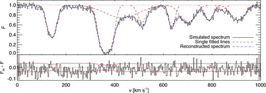
Decomposition of the Lyα forest in individual absorption lines. Top panel: the black histogram represents the Lyα absorption in a sight line from one of our models shown in velocity space. The average signal-to-noise level of this spectrum is 33.2. The red dashed curves are the individual fitted absorbers, whereas the total reconstructed absorption is shown as the blue dot–dashed curve. The red dotted line follows the continuum (F = 1). Bottom panel: the deviation of the reconstructed flux Ffit from the original spectrum F, compared with the assumed noise level for this synthetic spectrum (delimited by the red solid lines). Overall, the combined fit is a good approximation to the original spectrum, except in regions characterized by flat absorption profiles (for example around v = 200–300 km s−1), which cannot be decomposed into individual lines. Note also that rather broad lines are sometimes required to reproduce the absorption profile, which are not obviously interpretable as single absorbers (e.g. in the case of the line centred around v ∼ 450 km s−1). The parameters of these broad lines are also particularly sensitive to systematic uncertainties due to the continuum placement.
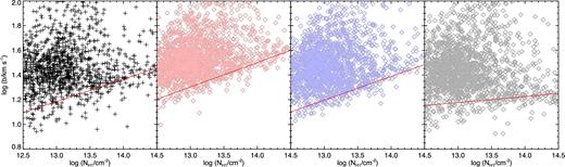
Distributions in the log NHI–b plane for the lines fitted in the quasar data sample (left-hand panel) and in three IGM models with T0 = 25000 K, γ = 1.6 (centre left-hand panel), T0 = 15000 K, γ = 1.6 (centre right-hand panel) and T0 = 15000 K, γ = 1 (right-hand panel). All three models have smoothing parameter ξ = 0.8, corresponding to a smoothing length λP = 93 kpc (comoving). The red solid lines represent the fitted power law to the cut-off of the distribution, which is sensitive to the thermal parameters of the IGM. The behaviour of these lines in the three models illustrates the sensitivity of the cut-off to the thermal parameters, which has been used in the past to constrain the thermal parameters (e.g. Schaye et al. 1999; Rudie et al. 2012), and the difference in T0 between the second and third panels determines a clear change in the intercept of the fitted line. Conversely, the lower slope of the TDR used in the right-hand panel, which shows an isothermal model, makes the cut-off much flatter than in the other two cases.
4.1 The lower cut-off in the b–N distribution
As noted previously (Schaye et al. 1999; Theuns, Schaye & Haehnelt 2000; McDonald et al. 2001), the b–N distribution shows a pronounced cut-off at low values of b. This is usually interpreted as a signature of thermal broadening setting a lower limit to the absorption line widths. The position of this cut-off is dependent on the column density, suggesting that the temperature systematically varies with the density of the gas. This motivated several studies to use the slope and normalization of the lower of the b–N distribution as a direct probe of the TDR of the IGM. Pressure smoothing also broadens the lines by increasing the physical size of absorbers, which increases their velocity width due to the Hubble flow. This effect can be taken into account by means of theoretical/analytical arguments or hydrodynamics simulations (Schaye et al. 1999; Theuns et al. 2000; Garzilli, Theuns & Schaye 2015).
One may notice from Fig. 2 that the lines fitted in the data sample (left-hand panel) present more outliers below the cut-off compared to the models (right-hand three plots). To understand what could generate this difference, we visually inspected all individual absorbers in the data with width lower than the cut-off by more than log b = 0.1. Among 29 outliers, we found 7 that are compatible with being unidentified metal lines and other 7 that are Lyα absorbers associated with metals at the same redshift. The latters are metal-enriched systems whose temperature might be affected by metal cooling, which is not accounted for in our models. We have tested the effect of removing these 14 lines and to re-apply the cut-off fitting procedure. This did not significantly change the estimated cut-off parameters, but it reduced the uncertainty on log b0 by about 20 per cent. For this reason, we consider keeping all the outliers to be the most conservative choice.
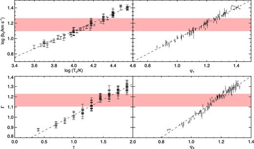
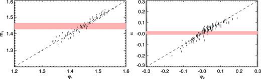
Calibrated relations between the parameters b0 and Γ describing the normalization and slope of the lower cut-off in the b–N distribution and the thermal parameters T0 and γ describing the TDR. Left-hand column: cut-off normalization log b0 at log NHi, 0/cm−2 = 13 as a function of log T0 (upper panel) and slope of the fitted Γ as a function of the index γ of the TDR (lower panel). Each point represents a different model in the grid and errors are estimated by bootstrapping the simulated line samples. The red bands delimit the values of log b0 and Γ measured from the data within the 1σ error. The calibrated function log b0(log T0) is obtained via a linear fit of these points (dashed lines). The two relations shown in this plot are reasonably tight, but the level of scatter appears higher than what the error bars warrant, suggesting that dependencies on other parameters are not negligible. This can have an effect on the inference of the thermal parameters. Right-hand column: same as the left-hand panel, but using the generalized combination of thermal parameters described in Section 4.2. Each point represents the mean of the MCMC posterior distribution for the combinations used to describe log b0 (upper panel) and Γ (lower panel). The (small) horizontal error bars represent the propagated uncertainties on the combination coefficients as obtained from the posterior distribution. The dashed lines represent the identity. Adopting the generalized scheme substantially improves the fits: the chi-square for the four plots, divided by the number of points, is 3.49 (top left-hand panel), 2.70 (top right-hand panel), 4.16 (bottom left-hand panel) and 2.56 (bottom right-hand panel).
In the next section, we discuss how we abandon these assumptions in order to include a more general relation between the parameters describing the lower cut-off of the b–N distribution and parameters describing the thermal state and history of the IGM, including the smoothing length λP.
4.2 Generalizing the calibration of the cut-off parameters
The relations described by equations (5) and (6) are based on the heuristic argument that the renormalization of the TDR changes the line widths at all column densities by a similar proportion, at least for lines that fall near the cut-off. Although Fig. 3 suggests that such an approximation is reasonable, we would like to consider the possibility of more general dependencies in order to find a scheme to quantify the effect of the pressure smoothing on the line distribution.
A convenient way of doing so is to implement a likelihood probability for fitting ϕ with ψ and to include it in a Markov chain Monte Carlo (MCMC) algorithm in the space of coefficients. This can be combined with a likelihood of the measured observable ϕd when compared to the value of ψ for a given choice of the coefficients and of the thermal parameters. This allows us to draw quantitative inferences on the calibration coefficients {a, b, c, d} and on the thermal parameters {T0, γ, λP} at the same time.
This scheme is computationally inexpensive and achieves several goals:
It generalizes the simple power-law calibration assumed in equation (5).
It finds the parameter combinations to which the observable is sensitive, providing a way to quantitatively express its degeneracy direction.
The uncertainty of this calibration can be determined based on the scatter of the simulated points and their uncertainties.
It returns the constraints on the thermal parameters, marginalizing over the uncertainty on the coefficients of equation (7).
The main drawback is that the validity of equation (7) as an approximation of the observable ϕ must be verified a posteriori, using the estimated coefficients from the MCMC run.
In the case where the observable ϕ is not a scalar but a vector, it is possible to generalize the likelihood expressions 8 and 9 to multivariate Gaussian likelihoods. This will increase the dimensionality of the calculation because there must be four coefficients {a, b, c, d} for each observable component. It will also be necessary to calculate the full covariance matrix of the different components of ϕ.
In this work, we have applied this formalism to the observables (log b0, Γ) that describe the lower cut-off of the b–N distribution and to the differential median parameters (m1, α) that we will define in the next section. In both cases, this involved an 11-parameter MCMC analysis and adopting a bivariate Gaussian likelihood, both for equation (8) and (9). The correlation between log b0 and Γ has been calculated by bootstrapping the sample of absorption lines, as it was done for the standard deviations.
4.3 Differential median of the line width distribution
Although the cut-off is certainly the most prominent feature of the distribution, it is reasonable to expect that the thermal properties of the IGM do not only affect the narrowest lines in the Lyα forest. Taking advantage of the additional information contained by the bulk of the line population is an obvious way of trying to refine the constraints achievable with a Voigt-profile decomposition approach. Some of our preliminary efforts to do so encountered systematic issues related to very broad lines (b > 60 km s−1). Our models were not able to reproduce the observed line distribution in that range, and, more problematically, inferences on the thermal parameters from various fitting schemes were strongly dependent on the way the upper b range was chosen or on the statistic employed to characterize the line distribution. We concluded that the broad lines are in most cases probably an artefact of the fitting procedure and do not represent physical properties of the IGM (see for example Fig. 1) and are therefore more subject to systematic errors, in particular, due to the uncertainty of the continuum placement.
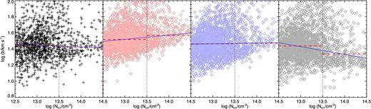
Representation of the differential median statistic. The points in the four panels show the b–N distribution of the data and the simulation for the same three thermal models as in Fig. 2. The vertical dotted lines separate the two |$N_{\rm H\, \small {I}}$| ranges for which the two medians m1 and m2 (shown in dashed red horizontal lines) are calculated. The blue lines describe the equation |$b=m_1^{\prime }-\alpha (\log N_{\rm H\, \small {I}} - 13)$| chosen so that they horizontally divide both column-density ranges into two parts with an equal numbers of points (see text for details). m1 and α are the two parameters used in the analysis. The plot illustrates their sensitivity to the thermal parameters γ and T0.
5 RESULTS
In the left-hand panels of Fig. 3, we show the values of log b0 in the simulations as a function of the temperature at mean density and Γ as a function of the slope of the TDR γ. When fitting the linear relations in equation (5), we obtain A = 2.06, B = 1.76; C = −0.07 and D = 3.28 (corresponding to the black dashed lines). The cut-off-fitting algorithm applied to the data returns log b0 = 1.186 ± 0.084 and Γ = 0.180 ± 0.062, marked as the red shaded region in the plot. By applying the above coefficients to convert these numbers to a measurement of the TDR parameters, we get T0/103 K = 14.3 ± 5.0 and γ = 1.52 ± 0.22. The reported uncertainties take into account the propagated (small) errors of the cut-off calibration coefficients.
The generalization of the relation between the thermal parameters T0 and γ, and the parameters characterizing the lower cut-off of the b–N distribution described in Section 4.2 is shown in the right-hand panels of Fig. 3. These plots are analogous to the left-hand panels except that the x-axes are combinations of the thermal parameters as defined in equation (7). The coefficients for equation (7) are picked from the mean values of the MCMC posterior distribution, applying the method described in Section 4.2 to a joint analysis of Γ and log b0. More precisely, the average combinations are ψ1 = −1.03 + 0.55 log T0 − 0.02(γ − 1) − 0.02 log λP and ψ2 = 0.10 − 0.06 log T0 + 0.27(γ − 1) + 0.09 log λP. These relations do not represent a new ‘calibration’ in which the coefficients are free to vary consistently with the uncertainties on the values extracted from the simulations. However, showing that the relations between the observables and the typical combinations from the MCMC fall close to the identity relation (dashed line) is necessary to validate our approach. The constraints on the thermal parameters derived from the same MCMC analysis are shown in the green contour plots in Fig. 6. A degeneracy between the inferred values of T0 and γ is evident, which is a consequence of taking the statistical correlation between the measured Γ and log b0 into account. The right-most panel demonstrates that the lower cut-off in the simulated b–N distribution is not sensitive to the smoothing length λP. When marginalized over all parameters of the MCMC analysis, including the coefficients for ψ1 and ψ2, the values inferred for the TDR parameters are T0/103 K = 15.6 ± 4.4 and γ = 1.45 ± 0.17 (quoted as mean and standard deviation from the posterior distribution). The uncertainties are smaller than those inferred from the lower cut-off, and the two measurements are in good agreement.
The results obtained from the differential median technique are presented in Fig. 5. The two panels show that the quantities m1 and α are reasonably approximated by a combination of the form of equation (7), although the scatter is not negligible. As in Fig. 3, the red bands trace the 1σ limits for the measured parameters: m1 = 1.446 ± 0.020 (left-hand panels) and α = 0.007 ± 0.016. The relations are well described by ψ1 = −0.433 + 0.256 log T0 + 0.038(γ − 1) + 0.409 log λP and ψ2 = 0.285 − 0.141log T0 − 0.194(γ − 1) + 0.200 log λP. The posterior distribution of the thermal parameters, shown as blue contours in Fig. 6, reveals degeneracies between the inferred values of all three considered parameters. In particular, and in contrast to the cut-off method, there is a significant sensitivity to the pressure smoothing length λP. This confirms that the overall b–N distribution contains information about the spatial smoothing of the IGM gas, as already noted by Garzilli et al. (2015). The marginalized uncertainties for the TDR parameters are in this case T0/103 K = 14.6 ± 3.7 K and γ = 1.37 ± 0.17, in good agreement with those inferred from the lower cut-off of the b–N distribution. The fact that using the full distribution does not substantially improve the accuracy of the constraints, compared to using just the lower cut-off, is due to the degeneracy with λP, which was negligible for the lower cut-off method. On the other hand, the emergence of such degeneracy implies that the precision can be substantially improved by combining these results with independent measurement of the smoothing length. At the moment, the only constraints available on λP are those obtained by the analysis of correlated Lyα absorption in close quasar pairs (Rorai, Hennawi & White 2013; Rorai et al. 2017a). The horizontal bars in Fig. 6 represent the result from Rorai et al. (2017a) in the redshift bins 2.2–2.7 (red) and 2.7–3.3 (black), both overlapping with the redshift range analysed in the present work. The nominal value of the λP measurement has been decreased by 10 per cent, in order to match the definition of pressure smoothing as given by the Freal cut-off (see section 3.1 and fig. S11 in Rorai et al. 2017a). As it can be seen, the whole range for λP considered in this paper is consistent with either of the two data points. More precise measurements of the smoothing, or an analysis conducted on the same redshift limits used in this work, are required in order to break the degeneracy and improve the accuracy on T0 and γ achievable with the differential median technique.
Same as Fig. 3 (right-hand column), but for the differential median method, showing the relation between the low-column-density median m1 and the differential coefficients α with the respective average parameter combinations obtained by the MCMC analysis, ψ1 and ψ2.
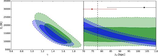
Constraints on the thermal parameters from the two analyses presented in this work. In green we show the 1σ (dark) and 2σ (light) confidence levels in the T0–γ and T0–λP planes, derived from the cut-off method. The analysis takes into account the statistical correlation between the uncertainties of the two observables, log b0 and Γ. Mainly due to this correlation, there is a strong degeneracy between the estimated values of T0 and γ, although the marginalized uncertainty of the two parameters of the TDR is comparable to the one achieved in the standard method. The right-hand panel shows that the temperature T0 inferred from the lower cut-off of the b–N distribution is not sensitive to the smoothing scale λP of the numerical simulations used for calibration. The blue contours are the 1σ (dark) and 2σ (light) confidence levels for the differential median method. Similar to the analysis based on the lower cut-off of the b–N distribution, there is a strong degeneracy between the inferred T0 and γ; however, for this method, the temperature is also strongly degenerate with the smoothing length λP. The range for λP shown in this plot is consistent with recent measurements from Rorai et al. (2017a) at z ∈ 2.2–2.7 (shown as a red circle with errorbars) and z ∈ 2.7–3.3 (black, the vertical position of these two points is arbitrary). The vertical dashed line shows the value of λP measured in the non-equilibrium hydrodynamics model by Puchwein et al. (2015) at z = 2.79. Stronger constraints on the pressure smoothing will eventually help break the degeneracy shown in this plot and significantly improve the precision achievable with this technique.
An alternative way of visualizing our results is to look at the constraints in the temperature–density plane. This does not require us to reduce the posterior distribution to two parameters with relative uncertainties. It also allows a straightforward comparison with the measurement of the temperature at overdensity |$\bar{\Delta }$| obtained with the ‘curvature’ statistic in BB11 and Boera et al. (2014), without requiring error propagation by which some information might be lost. The way we do this is the following: given the posterior distribution for T0 and γ obtained from one of our MCMCs, we calculate the marginalized distribution of T0Δγ − 1 for the range of overdensities Δ we are interested in. We then plot the 16th and the 84th percentile as a function of Δ as the 1σ limits in the temperature–density plane. The results for the various techniques described in this paper are shown in Fig. 7. The black dotted lines show the 16th and 84th percentiles of the temperature distributions obtained from the lower cut-off MCMC analysis, whereas the red shaded region shows the same for the differential median method. Note that the curvature results do not include uncertainties related to pressure smoothing. There is good agreement between the two measurements, and there is also good consistency with the results from BB11 and Boera et al. (2014) at the same redshift (red square and pentagon, respectively), although our data set partially overlap with the sample used in Boera et al. (2014). Note that the uncertainties of the temperature measured with the median technique are lower at mild overdensities (Δ ∼ 2.5–3.5) than at the mean density. This is a consequence of the particular degeneracy direction in the T0–γ plane of Fig. 5.
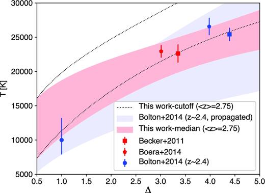
Constraints on the TDR in the temperature–density plane. The black dashed lines show the 16th and 84th percentile of the temperature posterior distribution as a function of density, obtained from our analysis of the lower cut-off of the b–N distribution. Analogous limits for the differential median method are shown by the red shaded area. The two measurements are in good agreement with each other. The red square and pentagon report the measurements of T(Δ) at the same redshift from BB11 and Boera et al. (2014), respectively. For comparison, we also report the results for T0 at z = 2.4 from Bolton et al. (2014) (blue circle) and the propagated 1σ limits at all densities considering the measurement of γ from the same work (light blue shaded area). The blue square and pentagons are the values of T(Δ) obtained in BB11 and Boera et al. (2014) at this redshift.
For reference, we also show an analogous comparison at z = 2.4 between the results of BB11 (blue square), Boera et al. (2014) (blue pentagon) and b-|$N_{\rm H\, \small {I}}$| cut-off results from Bolton et al. (2014) (blue circle). These limits assume that T0 and γ are uncorrelated, which is likely incorrect given the results of our analysis at slightly higher redshifts. The light blue shaded area in the background represent the propagated 1σ limits on T(Δ), assuming the measured value and uncertainties of T0 and γ from Bolton et al. (2014).
6 DISCUSSION
A more comprehensive comparison of the main results of this work with recent constraints on the thermal state of the IGM from the literature is presented in Fig. 8, where we show the evolution of T0 (upper panel) and γ (lower panel) as a function of redshift. The red triangles correspond to the constraints from our fit to the lower cut-off of the b–N distribution (Section 4.2), whereas the red squares are those obtained from the differential median method (Section 4.3). The black solid lines are the predictions of a recent hydrodynamics simulation from Puchwein et al. (2015), where the UV background is assumed to follow the model by Haardt & Madau (2012). This simulation fits well both the observational points from this work and those reported by Bolton et al. (2014) (blue circles). If we assume a slope of the TDR as in the Puchwein et al. (2015) simulation, (i.e. the black line in the lower panel), we can extrapolate the curvature measurements of T(Δ) (BB11, Boera et al. 2014) to mean density. The corresponding values of T0 are shown as the dark blue connected circles for BB11, and the orange connected triangles for an updated version of the results of Boera et al. (2014) and Boera, private communication. The good agreement of our measurements of T0 and the evolution of T0 inferred from the extrapolation of the temperature measurements with the curvature method to mean density based on the γ values predicted by the Puchwein et al. (2015) simulation is a non-trivial result that suggests that our understanding of the thermal state IGM is converging from multiple different approaches. Convergence of results is also suggested by the measurements of T0 obtained with a wavelet-analysis technique by Lidz et al. (2010) (cyan triangles) and Garzilli et al. (2012) (grey pentagons). The discrepancy with their measurements in the redshift bins close to that of our measurement is less than 1σ.
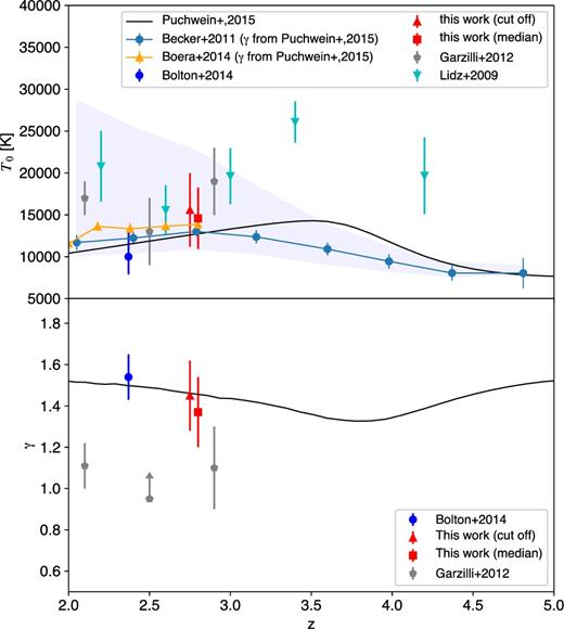
A summary of recent constraints on the TDR parameters from the literature, as a function of redshift. Our constraints on T0 and γ derived from the lower cut-off of the b–N distribution (red triangles) and the differential median (red squares) methods are compared to the hydrodynamics model of Puchwein et al. (2015, black line) and the extrapolated values of T0 from the curvature measurement of BB11 (dark blue connected circles). The latter values are obtained from the temperatures at a redshift-dependent overdensity |$\bar{\Delta }(z)$| by assuming the value of γ from the Puchwein et al. (2015) model (black line in the lower panel). The light-blue shaded area represents the range of values extrapolated from BB11 assuming a flat prior on γ in the interval 1–1.6. We also plot the constraints from Bolton et al. (2014, blue circles) at somewhat lower redshift. The orange triangles are the values of T0 extrapolated from a recalibrated version of the curvature measurement from Boera et al. (2014) and Boera (private communication), obtained in the same way as for BB11. The cyan triangles show the constraints on T0 from Lidz et al. (2010) and the grey pentagons those from Garzilli et al. (2012), both obtained with a wavelet analysis (combined with the flux PDF in the latter). The grey pentagons in the lower panel are also from the PDF-Wavelet combined analysis of Garzilli et al. (2012). The tension between the points at z = 2.9 with our measurements is discussed in the text.
In the lower panel, the measurement of γ at z = 2.9 derived from a joint analysis of the flux PDF and the wavelet coefficients (Garzilli et al. 2012) is clearly in tension with our work presented here and the analysis of Bolton et al. (2014). As discussed earlier, other measurements based on the flux PDF (e.g. Viel et al. 2009; Calura et al. 2012) also have claimed that an ‘inverted’ TDR (γ < 1) is required to match the data (but see Lee 2012; Rollinde et al. 2013; Lee et al. 2015). This apparent discrepancy has been recognized for some time and was recently discussed in considerable detail by Rorai et al. (2017b). By analysing a high signal-to-noise quasar spectrum at z = 3, Rorai et al. (2017b) confirmed that the flux PDF constrains the TDR to be flat or to rise towards low density; however, as they point out, this is true only for gas around and below the mean density, to which the PDF statistic is most sensitive. Rorai et al. (2017b) further show that techniques for measuring the IGM temperature that rely on quantifying the smoothness of the absorption profile, such as those discussed in this paper or the curvature method developed by B11, are mainly sensitive to overdense gas, i.e. Δ > 1. This has also been highlighted in Bolton et al. (2014), where they show the relation between column density and optical depth-weighted density (see fig.1 in their paper). The fact that our work presented here constrains a spatially invariant TDR to have γ > 1 corroborates the conclusion of Rorai et al. (2017b) that a single, spatially invariant power law is not able to describe the TDR of the low density IGM. This may perhaps be explained by simulations of He ii reionization where radiative transfer effects have been implemented (Abel & Haehnelt 1999; Paschos et al. 2007; McQuinn et al. 2009; Compostella, Cantalupo & Porciani 2013; La Plante et al. 2017), in which the lower densities show a bimodal temperature distribution with increased temperatures and a flattening of the relation between temperature and density in regions where helium has most recently become doubly ionized.
Finally, we note that in a recent work, Garzilli et al. (2015) found that the cut-off of the line distribution is significantly sensitive to the pressure smoothing, different from what our analysis shows (see Fig. 6). This could be possibly due to the differences in the fitting algorithms, both for the individual Lyα lines and for the cut-off, but it is most likely related to the particular range of column density we have selected. Fig. 8 in their paper suggests that the effect of pressure smoothing on the low-b lines is most prominent for lines with low column densities, whereas here we have considered only those with |$N_{\rm H\, \small {I}}>10^{12.5}$| cm−2, for which the line width is dominated by thermal broadening, as argued also by Bolton et al. (2014).
7 CONCLUSIONS
We have analysed the Lyα forest of a sample of 13 high-resolution quasar spectra in the redshift range 2.55 < z < 2.95 with the help of high resolution numerical simulations of the IGM. The continuum-normalized spectra were decomposed into individual H i absorbers using vpfit, and we have carefully identified and excluded regions potentially contaminated by metal lines. We have then used the lower cut-off in the |$b\text{--}N_{\rm H\, \small {I}}$| distribution and a newly introduced statistic based on the medians of the line-width distribution in separate column density ranges to obtain two new measurements of the temperature of the IGM. In both cases, we employed Bayesian MCMC techniques to constrain thermal parameters, using a grid of thermal models where the TDR has been imposed in post processing. Our results can be summarized as follows.
Fitting the lower cut-off of the b–N distribution in the standard way gives T0/103 K = 14.3 ± 5.0 K and γ = 1.52 ± 0.22.
The parameters describing the lower cut-off and that describing the TDR are strongly correlated in simulations, but there is significant scatter due to the residual dependence on other thermal parameters (in particular, the smoothing length λP).
We have introduced a new calibration of the temperature measurement based on a linear combination of the thermal parameters (in logarithmic space) whose coefficients are left free to vary. For this new calibration, we have implemented an MCMC analysis in which the calibration coefficients are estimated together with the thermal quantities T0, γ and λP.
Including the correlation between the statistical uncertainties of log b0 and Γ in our likelihood, analysis gives T0/103 K = 15.6 ± 4.4 K and γ = 1.45 ± 0.17. Taking the correlation between T0 and γ shows that the inferred values for the two parameters are strongly degenerate. Conversely, no sensitivity is found to the smoothing length λP.
We have introduced an alternative statistical estimator for the thermal parameters which is based on the medians m1 and m2 of the line-width distribution for N < 1013.5 and N > 1013.5 cm−2, respectively. For this, we have defined the transformation |$\log b^{\prime }=\log b + \alpha (\log N_{\rm H\, \small {I}} - 13)$|, with α chosen such that m1 = m2 for b΄.
By applying the parameters m1 and α to the same MCMC technique used for the lower cut-off method, we obtain T0/103 K = 14.6 ± 3.7 K and γ = 1.37 ± 0.17, in good agreement with our measurement from the lower cut-off. For the measurement based on the differential median method, we find a strong degeneracy with the smoothing length λP, suggesting, unsurprisingly, that the overall b–N distributions contains information about the small-scale spatial structure of the IGM.
When we use the posterior distribution for the TDR parameters to infer the temperature at Δ ≈ 3, we obtain values consistent with the measurements at the same redshift from BB11 and Boera et al. (2014).
Our measurements are also in good agreement with the theoretical predictions from the hydrodynamics model of Puchwein et al. (2015) and with the measurements of T0 at similar redshifts from Lidz et al. (2010) and Garzilli et al. (2012).
Our constraints on γ are in disagreement with claims of an inverted TDR based on the flux PDF, similar to published results using statistics based on the smoothness of the absorption. Our findings further corroborate those of Rorai et al. (2017b), who argued that this is due to the different overdensity range probed by the PDF.
The work presented here marks a further step towards a consistent characterization of the thermal state of the IGM at z ≲ 3. The agreement with other recent measurements at the same redshift and with high resolution hydrodynamics models is an encouraging sign that our understanding of the thermal state of the IGM is converging. The techniques developed and presented here can be easily applied to data sets at other redshifts and should improve the well-established approach of characterizing the thermal state of the IGM with help of the b–N distribution of Lyα forest absorbers. Our analysis takes into account the uncertainties in the calibration between the lower cut-off (or the median b-parameters in different column density ranges) and the thermal parameters, as well as parameter correlations and second-order dependencies which were previously neglected. The degeneracies we find, especially in our analysis based on the differential median, suggest that a joint analysis with different statistics constraining the pressure smoothing length will significantly improve the precision of current constraints on the thermal state of the IGM.
ACKNOWLEDGEMENTS
We are grateful to W.L.W. Sargent for kindly providing two of the spectra analysed in this work, Volker Springel for making gadget-3 available and Girish Kulkarni for sharing the code for the calculation of λP in SPH simulations. We thank the anonymous referee for useful comments and suggestions, which greatly improved this manuscript. MH acknowledges support by ERC ADVANCED GRANT 320596 ‘The Emergence of Structure during the epoch of Reionization’. GDB was supported by the National Science Foundation through grant AST-1615814. JSB acknowledges the support of a Royal Society University Research Fellowship. MTM thanks the Australian Research Council for Discovery Project grant DP130100568. This work made use of the DiRAC High Performance Computing System (HPCS) and the COSMOS shared memory service at the University of Cambridge. These are operated on behalf of the STFC DiRAC HPC facility. This equipment is funded by BIS National E-infrastructure capital grant ST/J005673/1 and STFC grants ST/H008586/1, ST/K00333X/1.
Footnotes
In reality the average transmission of the Lyα forest evolves throughout this redshift bin. We have verified, however, that modelling the forest using a single value for the mean flux over this redshift range has only a small effect on the results when compared to the statistical uncertainties (see appendix).
REFERENCES
APPENDIX: EFFECT OF TEMPERATURE AND OPTICAL DEPTH VARIATION
To understand the effect of an evolving optical depth and a possible variation in temperature, we conducted the following test:
We created a model which is a mixture of four models with different effective optical depth, |$\tau _{\rm eff}=-\log \bar{F} = 0.33, 0.3, 0.29, 0.27$|. This values encompass the evolution of the mean transmission across our redshift bin.
We created another model which is a mixture of three models with different temperatures at mean density T0 = 10 000, 15 000, 20 000 K. This mixture could be interpreted either as a (rather extreme) temperature evolution with redshift or as spatial fluctuations.
We then calculated the cut-off and the differential median statistic for the two mixed models and for their individual components. The results are shown in Fig. A1.
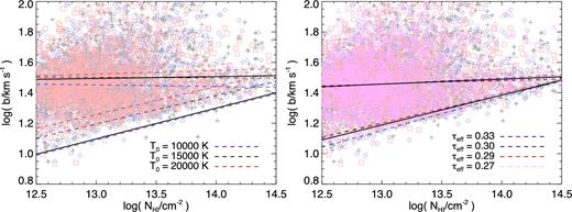
Effect of mixed temperatures or effective optical depths on the cut off and on the differential median. Left-hand panel: a combination of three models with T0 = 10 000 K (blue diamonds and lines), T0 = 15 000 K (black crosses and lines) and T0 = 20 000 K (red squares and lines). The differential median is represented as in Fig. 4, by dashed lines for the individual models and by a thick solid black line for the combination of all of them. The same is done for the lower cut-off. Right-hand panel: same as the left-hand panel, but for a combination of four models with different effective optical depth τ = 0.33 (blue) τ = 0.30 (blue) τ = 0.29 (blue) τ = 0.27 (blue).
In the case of the optical depth mixture (right-hand panel), the differences between the total model (black solid lines) and the four components (coloured dashed lines) are minimal, especially for the differential median statistic. One of the four cut-offs slightly deviates from the others at low column densities, but given that there is no clear trend and given the magnitude of the error (the outlier model has an uncertainty of Δlog b0 = 0.065, four times larger than the other models), we consider it a statistical fluctuation due to the noise/bootstrap realizations.
In the case of the temperature mixture (left-hand panel), it appears evident that the differential median of the total model (black solid) depends on the average temperature, i.e. coincides with the middle of the three components, whereas the cut-off picks the coldest of the three. This suggests that if there is significant temperature evolution or fluctuation, measurements based on the cut-off will be biased towards the lower values, differently from the median statistic. However, our measurements based on the two methods are in good agreement, and if anything, the cut-off analysis points towards slightly higher temperatures, which leads us to conclude that this effect is negligible at this level of precision.
