


Abstract
In this paper, we study a set of 12 pulsars that previously had not been characterized. Our timing shows that eleven of them are ‘normal’ isolated pulsars, with rotation periods between 0.22 and 2.65 s, characteristic ages between 0.25 Myr and 0.63 Gyr, and estimated magnetic fields ranging from 0.05 to 3.8 × 10¹² G. The youngest pulsar in our sample, PSR J0627+0706, is located near the Monoceros supernova remnant (SNR G205.5+0.5), but it is not the pulsar most likely to be associated with it. We also confirmed the existence of a candidate from an early Arecibo survey, PSR J2053+1718, its subsequent timing and polarimetry are also presented here. It is an isolated pulsar with a spin period of 119 ms, a relatively small magnetic field of 5.8 × 10⁹ G and a characteristic age of 6.7 Gyr; this suggests the pulsar was mildly recycled by accretion from a companion star, which became unbound when that companion became a supernova. We report the results of single-pulse and average Arecibo polarimetry at both 327 and 1400 MHz aimed at understanding the basic emission properties and beaming geometry of these pulsars. Three of them (PSRs J0943+2253, J1935+1159 and J2050+1259) have strong nulls and sporadic radio emission, several others exhibit interpulses (PSRs J0627+0706 and J0927+2345) and one shows regular drifting subpulses (J1404+1159).
1 INTRODUCTION AND MOTIVATION
Since the discovery of the first radio pulsar in 1967 (Hewish et al. 1968), more than 2500 rotation-powered pulsars have been discovered (Manchester et al. 2005). Of these, more than 400 have been ‘left behind’, – that is, they have no published phase-coherent timing solutions, so that we lack a rudimentary knowledge of their proper motions, spin-down parameters (including characteristic age, magnetic field, spin-down luminosity) and possible orbital elements. Similarly, no polarimetry and fluctuation spectral analyses have been done for many pulsars, and for many of these even basic quantities such as flux densities, rotation measures (RMs) and spectral indices are lacking. Because of this, the scientific potential for many of these objects is simply unknown and unexploited.
In this and subsequent papers, we attempt a partial remedy to this situation by characterizing some of these pulsars: We present their timing solutions (with derivations of characteristic ages, surface magnetic field and rotational spin down) and study some of their radio emission properties. As for all previously well characterized pulsars, the measurements presented here and in subsequent papers will aid future studies of the pulsar population and contribute to the understanding of their emission physics.
In this first paper, we focus on a group of a dozen pulsars discovered with the 430-MHz line feed of the Arecibo 305-m radio telescope in Puerto Rico before the Arecibo upgrade, i.e. pulsars that were found more than 20 yr ago, but were then never followed up. Most pulsars in this group were discovered in drift-scan surveys: two, J0943+22 and J1246+22, were reported by Thorsett et al. (1993) and three others (J0435+27, J0927+23, J0947+27) were discovered in the completion of that survey by Ray et al. (1996). Five further pulsars (J0517+22, J0627+07, J1404+12, J1935+12 and J1938+22) were discovered in the Arecibo–Caltech drift-scan survey (Chandler 2003), but again no timing solutions were presented for any of them. Two of these pulsars were later timed by other authors: J0627+0706, which we timed from 2005 February 17 to November 1, was detected by the Perseus Arm pulsar survey and subsequently timed from 2006 January 1 to 2011 May 9 (Burgay et al. 2013). Their timing results are similar to ours, but more precise given the larger timing baseline. J1938+22, which we did not follow up, was later timed by Lorimer, Camilo & McLaughlin (2013), so that it is now known as J1938+2213.
Two other pulsars (J1756+18 and J2050+13) were discovered in the Arecibo 430-MHz Intermediate Latitude (pointed) Survey (Navarro et al. 2003); they were reported in the Navarro et al. paper describing that survey, but without timing solutions because, although they were originally detected on 1990 July 19 and 1990 July 13 respectively, they were confirmed until 2003 January.
Finally, in Ray et al. (1996), an additional pulsar candidate (J2052+17) was listed, but the authors were unable to confirm it because of the start of the Arecibo upgrade. The candidate had a spin period P of 119.26 ms and a dispersion measure (DM) of 25 ± 3 cm− 3 pc. In 2004 October, we confirmed the existence of this pulsar using the 327-MHz Gregorian receiver of the 305-m Arecibo radio telescope and the wideband arecibo pulsar processors (WAPPs, Dowd, Sisk & Hagen 2000) as back-ends. Both the topocentric spin period (119.27 ms) and DM of 27 cm− 3 pc were compatible with the parameters in Ray et al. (1996). The pulsar has an exceptionally narrow profile, which represents less than 1 per cent of a rotation cycle, as presented in Fig. 1, and in more detail in Fig. 14.
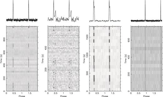
Grey-scaled intensity plots (with darker shade implying a larger intensity) showing total intensity of the pulsed signal at a frequency of 327 MHz as a function of spin phase (two spin cycles shown for clarity) and time. During many time segments, the pulsed signal of PSRs J0943+2253, J1935+1159 and J2050+1259 (but not PSR J2053+1718) disappears, i.e. the first three pulsars null. The right-hand plot shows the remarkably narrow pulse profile of PSR J2053+1718.
In what follows, we present detailed studies for these objects, both of their timing and emission properties. In Section 2, we briefly discuss the timing observations and their results; Section 3 describes the pulse-sequence, profile and polarization analyses; Section 4 discusses the origin of PSR J2053+1718; and Section 5 summarizes the various results.
2 TIMING OBSERVATIONS AND RESULTS
The aforementioned pulsars are relatively bright, and for that reason, they were used as test pulsars during the very early demonstration stages of the Arecibo 327-MHz drift scan survey (AO327, Deneva et al. 2013). These observations were carried out with the 327-MHz Gregorian feed and one of the four WAPPs as backends. They all were acquired in search mode, with 256 spectral channels, a sampling time of 64 μs and a bandwidth of 50 MHz. They were later dedispersed and folded using the presto routine ‘prepfold’ (Ransom, Eikenberry & Middleditch 2002), and then topocentric pulse times of arrival (TOAs) were derived from the resulting profiles using the Fast Fourier Transform technique described by Taylor (1992) and implemented in the presto routine get_TOAs.py.
At a later phase (2015/2016), we have used some of these pulsars (J0517+2212, J0943+2253, J1246+2253, J1404+1159 and J1935+1159) as test pulsars during follow-up sessions of AO327 discovered pulsars. These observations were made using the same 327-MHz Gregorian feed, but with the Puerto Rican Ultimate Pulsar Processing Instrument (PUPPI), which is a clone of the Greenbank Ultimate Pulsar Processing Instrument (GUPPI).1 Initial observations consisted of incoherent search mode observations with 69 MHz of bandwidth that was split into 2816 channels with a sample time of 81.92 μs. These data were dedispersed and folded using the fold_psrfits routine from the psrfits_utils software package.2 Later observations were performed using PUPPI in coherent fold mode with the same 69 MHz of bandwidth split into 44 frequency channels and were written to disc every 10 s. Radio Frequency Interference (RFI) was excised from both incoherent and coherent PUPPI files using a median-zapping algorithm included in the psrchive software package (van Straten, Demorest, & Oslowski 2012),3 and topocentric TOAs were derived using psrchive's pat tool.
The TOAs were then analysed using tempo,4 with the DE405 Solar system ephemeris;5 from this we derive a timing solution, where we can assign the correct integer rotation number to each pulse.
The characteristics of the timing observations are given in Table 1, together with the number of TOAs derived for each, the root mean square (rms) of the residuals (a residual is the measured TOA minus the prediction of the timing solution for the time of the respective pulse; as an example, we depict graphically the residuals of PSR J2053+1718 in Fig. 2) and the reduced χ2 of each fit. For some pulsars, this is much larger than 1, implying either the presence of effects that have not been modelled in their timing solutions, such as timing noise or pulse jitter, or that for some reason the TOA uncertainties were highly underestimated. The table also gives the new names for these pulsars, which are used throughout the remainder of this paper.
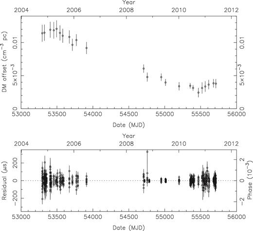
Top plot: DM offset (from 26.979 cm−3 pc) observed as a function of epoch for PSR J2053+1718. Bottom plot: residuals as a function of epoch for the same pulsar. No trends are noticeable in the timing.
Pulsar names (old and new), references and the parameters of our timing observations.
| Previous name | Reference | New name | Start | Finish | NTOA | rms | Reduced |
|---|---|---|---|---|---|---|---|
| (MJD) | (MJD) | (ms) | χ2 | ||||
| J0435+27 | Ray et al. (1996) | J0435+2749 | 52854 | 53785 | 96 | 0.12 | 14.38 |
| J0517+22 | Chandler (2003) | J0517+2212 | 53418 | 57701 | 518 | 0.12 | 7.9 |
| J0627+07a | Chandler (2003) | J0627+0706 | 53418 | 53675 | 91 | 0.26 | 22.82 |
| J0927+23 | Ray et al. (1996) | J0927+2345 | 53318 | 53910 | 26 | 0.47 | 0.77 |
| J0943+22 | Thorsett et al. (1993) | J0943+2253 | 53318 | 57876 | 731 | 0.17 | 2.57 |
| J0947+27 | Ray et al. (1996) | J0947+2740 | 53318 | 53910 | 35 | 0.28 | 1.88 |
| J1246+22 | Thorsett et al. (1993) | J1246+2253 | 53294 | 57876 | 448 | 0.22 | 4.28 |
| J1404+12 | Chandler (2003) | J1404+1159 | 53309 | 57380 | 335 | 0.62 | 12.78 |
| J1756+18 | Navarro, Anderson & Freire (2003) | J1756+1822 | 52645 | 53307 | 89 | 1.23 | 26.09 |
| J1935+12 | Chandler (2003) | J1935+1159 | 53306 | 57504 | 145 | 2.51 | 1.04 |
| J2050+13 | Navarro et al. (2003) | J2050+1259 | 52636 | 53306 | 27 | 8.81 | 1419.67 |
| J2052+17b | Ray et al. (1996) | J2053+1718 | 53295 | 56837 | 728 | 0.028 | 1.34 |
aSee also Burgay et al. (2013).
bPrevious unconfirmed candidate.
The timing solutions are presented in Table 2, which include precise measurements of right ascension and declination (this is the origin of the new names in the preceding table) the rotation frequency (ν), its derivative (|$\dot{\nu }$|) and DM. The reference epoch for all timing parameters is MJD = 53400. For these measurements, we have multiplied the TOA uncertainties by the square root of the reduced χ2 in Table 1, which yields a new reduced χ2 of 1.0. This procedure results in conservative estimates of the uncertainties of the timing parameters. These might still be in error due to the presence of correlated noise in the TOAs, such as that produced by timing noise; this is particularly important for PSRs J0627+0706, J1756+1822 and especially PSR J2050+1259.
Parameters from the timing solution for the reference epoch MJD = 53400. The digits in parentheses indicate the 1σ uncertainty estimated by tempo on the last digit of the value.
| Pulsar Name | Right ascension | Declination | ν | |$\dot{\nu }$| | DM |
|---|---|---|---|---|---|
| hhmmss.ss | ° ΄ ″ | (Hz) | (10−16 Hz s−1) | (pc cm−3) | |
| J0435+2749 | 04 35 51.818(4) | 27 49 01.7(4) | 3.064 857 408 039(13) | −0.767(10) | 53.19(2) |
| J0517+2212 | 05 17 17.147(2) | 22 12 51.9(2) | 4.497 079 963 269(13) | −2.3469(3) | 18.705(14) |
| J0627+0706 | 06 27 44.217(2) | 07 06 12.7(11) | 2.101 396 0823(5) | −1314.8(4) | 138.29 |
| J0927+2345 | 09 27 45.26(5) | 23 45 10.7(12) | 1.312 526 746 25(15) | −5.26(6) | 17.24(12) |
| J0943+2253 | 09 43 32.3975(10) | 22 53 05.66(4) | 1.876 261 648 496(3) | −3.16238(7) | 27.2508(15) |
| J0947+2740 | 09 47 21.287(18) | 27 40 43.5(2) | 1.1750 690 7189(7) | −5.94(3) | 29.09(7) |
| J1246+2253 | 12 46 49.363(5) | 22 53 43.27(8) | 2.110 280 928 271(14) | −3.9586(4) | 17.792(3) |
| J1404+1159 | 14 04 36.961(3) | 11 59 15.36(10) | 0.377 296 025 592(4) | −1.95656(16) | 18.466(9) |
| J1756+1822 | 17 56 17.583(8) | 18 22 55.3(2) | 1.344 084 323 77(12) | −9.27(3) | 70.80 |
| J1935+1159 | 19 35 16.076(14) | 11 59 09.2(4) | 0.515 528 177 82(4) | −2.5190(15) | 188.76(6) |
| J2050+1259 | 20 50 57.21(14) | 12 59 09(3) | 0.818 987 4162(6) | −3.38(15) | 52.40 |
| J2053+1718 | 20 53 49.4809(7) | 17 18 44.662(13) | 8.384 495 643 240(8) | −0.2014(7) | 26.979 |
Finally, the derived parameters are given in Table 3: Galactic coordinates (l, b) and distance (D); the latter is derived from the DM using two models of the electron distribution in the Galaxy (the NE2001 model, Cordes & Lazio 2002, and the YMW16 model, Yao, Manchester & Wang 2017), the spin period (P), its derivative (|$\dot{P}$|), the characteristic age (τc), magnetic field (B0) and spin-down energy (|$\dot{E}$|). The expressions for these quantities were adopted from Lorimer & Kramer (2005): |$\tau _{\rm c} = P / (2 \dot{P})$|, |$B = 3.2 \times 10^{19} \sqrt{P \dot{P}}$| and |$\dot{E}\, =\, 4 \pi ^{2} \, I \, \dot{P}/P^{3}$|, where I is the moment of inertia of the neutron star, which is generally assumed to be 1045 g cm2. All pulsars in the list are isolated, and most of them belong to the ‘normal’ group, with fairly typical rotation periods (between 0.22 and 2.65 s), characteristic ages (between 0.25 Myr and 0.63 Gyr) and B-fields (from 0.05 to 3.8 × 10¹² G). We now discuss the characteristic of the two extreme objects in our sample.
Derived parameters. The digits in parentheses indicate the 1σ uncertainty estimated by tempo on the last digit of the value. D1 is calculated using the NE2001 model and D2 is calculated using the YMW16 model. The asterisks indicate that the DM is larger than the model prediction for the total Galactic column density for the pulsar's line of sight.
| Pulsar name | Galactic coordinates | P | |$\dot{P}$| | log10(τc) | log10(B0) | D1 | D2 | |$\log _{10} \dot{ E}$| | |
|---|---|---|---|---|---|---|---|---|---|
| ℓ | b | (s) | (10−15 s s−1) | (τc in yr) | (B0 in G) | (kpc) | (kpc) | (|$\dot{E}$| in erg s−1) | |
| J0435+2749 | 171.8 | −13.1 | 0.326 279 453 4509(14) | 0.008 16(11) | 8.8 | 10.7 | 1.8 | 1.5 | 31.0 |
| J0517+2212 | 182.2 | −9.0 | 0.222 366 515 1983(6) | 0.011 6045(15) | 8.5 | 10.7 | 0.66 | 0.16 | 31.5 |
| J0627+0706 | 203.9 | −2.0 | 0.475 874 114 55(11) | 29.775(9) | 5.4 | 12.6 | 4.7 | 2.3 | 34.0 |
| J0927+2345 | 205.3 | +44.2 | 0.761 889 236 06(9) | 0.305(4) | 7.6 | 11.7 | 0.66 | 1.1 | 31.4 |
| J0943+2253 | 207.9 | +47.5 | 0.532 974 705 7409(7) | 0.089 831(2) | 8.0 | 11.3 | 1.2 | 3.5 | 31.4 |
| J0947+2740 | 201.1 | +49.4 | 0.851 013 803 30(5) | 0.430(2) | 7.5 | 11.8 | 1.28 | * | 31.4 |
| J1246+2253 | 288.8 | +85.6 | 0.473 870 557 518(3) | 0.088 891(9) | 7.9 | 11.3 | 1.5 | 2.5 | 31.5 |
| J1404+1159 | 355.1 | +67.1 | 2.650 438 732 91(3) | 1.374 45(11) | 7.5 | 12.3 | 1.4 | 2.2 | 30.4 |
| J1756+1822 | 43.8 | +20.2 | 0.744 000 939 76(6) | 0.5129(16) | 7.4 | 11.8 | 4.2 | * | 31.7 |
| J1935+1159 | 48.6 | −4.1 | 1.939 758 180 09(15) | 0.9478(6) | 7.5 | 12.1 | 6.8 | 8.7 | 30.7 |
| J2050+1259 | 59.4 | −19.2 | 1.221 019 9817(9) | 0.50(2) | 7.6 | 11.9 | 3.1 | 5.9 | 31.0 |
| J2053+1718 | 63.6 | −17.3 | 0.119 267 758 318 45(11) | 0.000 2864(10) | 9.8 | 9.8 | 1.9 | 2.1 | 30.8 |
2.1 PSR J0627+0706
With a characteristic age of only 250 kyr, PSR J0627+0706 is by far the most energetic object in this sample. This object displays a prominent interpulse, suggesting an orthogonal rotator. It also has significant timing noise, which is typical of young pulsars. This is the reason for the large reduced χ2 of its solution. This agrees with the results of Burgay et al. (2013).
Chandler (2003) remarked that this pulsar lies, in projection, within 3° of the centre of the old, large Monoceros supernova remnant (SNR G205.5+0.5), which is located at an RA of 06h 39m and Dec. of + 06° 30΄. For this reason, they proposed that if PSR J0627+0706 has a true age similar to that of SNR G205.5+0.5 (30 to 100 kyr, Leahy, Naranan & Singh 1986), it could be a candidate in association with that SNR. (They pointed out that the positional offset is possible given the age of the SNR and the proper motions of other pulsars observed in the Galaxy.)
The characteristic age, as measured by us and Burgay et al. (2013), for PSR J0627+0706 is larger by a factor of 2.5–8. However, this is not very constraining: True pulsar ages can be significantly smaller than their characteristic ages if they are born with a spin period similar to their current spin period.
Another way of verifying the association is through distance measurements. The estimated distance to the Monoceros SNR, 1.6 kpc (Odegard 1986), is less than the estimated DM distances to the pulsars NE 2001 (4.5 kpc) and YMW16 (2.3 kpc). Given the uncertainties in the DM models and their derived distances, this does not imply a distance inconsistency, particularly for the YMW16 model.
We note that this area of the Galaxy has an abundance of relatively young pulsars that could potentially be associated with SNR G205.5+0.5. In particular, the ‘radio-quiet’ gamma-ray pulsar PSR J0633+0632, discovered in data from the Fermi satellite (Abdo et al. 2009), was listed in the aforementioned paper as a ‘plausible’ association with SNR G205.5+0.5, based on its location within ∼1|$_{.}^{\circ}$|5 of the SNR centre. Later, Ray et al. (2011) measured the characteristic age of PSR J0633+0632 (59 kyr), which is also in agreement with the estimated age of the SNR. However, no radio emission has been detected yet in the latter pulsar, so its DM (and derived distance) is not yet known.
Despite that, we conclude that PSR J0633+0632 is more likely to be associated with SNR G205.5+0.5 than PSR J0627+0706.
2.2 PSR J2053+1718
PSR J2053+1718 has a much smaller spin period derivative and a much larger characteristic age than the other pulsars in this sample. A first simple fit for the parameters in Table 2 plus proper motion (see below) yields a reduced χ2 of 1.80, and visible trends in the residuals. Given the low frequency used in the timing and the relatively high precision of the measurements, these are likely due to variations in DM caused by the Earth's and the pulsar's movement through space. In order to measure the DM variation with time, we divided the 50-MHz bandwidth into four sub-bands, making separate TOAs for each sub-band. We then used the DMX model (Demorest et al. 2013) to measure the DM variations (displayed in Fig. 2) and subtract them; once this is done, the reduced χ2 decreases to 1.34.
The precise timing of this pulsar allows a measurement of its proper motion in right ascension and declination: μα = − 1.0(23) mas yr− 1 and μδ = + 6.9(28) mas yr− 1. These measurements are not highly significant, but they already represent a significant constraint on the transverse velocity vT. Given the DM distance estimates of 1.9 kpc (NE2001) and 2.1 kpc (YMW16), the proper motion implies vT = (63 ± 25) km s− 1 and (69 ± 28) km s− 1, respectively; this is typical of recycled pulsars (e.g. Gonzalez et al. 2011).
This proper motion allows for a correction of the observed |$\dot{P}$|, where we subtract the Shklovskii effect (Shklovskii 1970) and the Galactic acceleration of this pulsar relative to that of the Solar system, projected along the line of sight (Damour & Taylor 1991). (This was calculated using the latest model for the rotation of the Galaxy from Reid et al. 2014.) These terms mostly cancel each other, so that the intrinsic spin-down, |$\dot{P}_{\rm int} \, = \, 2.8 \times 10^{-19}\, \rm s \, s^{-1}$|, is very similar to the observed |$\dot{P}$|. This implies a low B-field of ∼ 5.8 × 10⁹ G and a characteristic age of ∼ 6.7 Gyr. The origin of this pulsar is discussed in Section 4.
3 PULSE-SEQUENCE AND PROFILE ANALYSES AND QUANTITATIVE GEOMETRY
Recently, we conducted single-pulse polarimetric observations on most of the above pulsars as well as a few others of related interest. The Arecibo observations were carried out at both the P band (327 MHz) and L band (1400 MHz) using total bandwidths of 50 MHz and typically 250 MHz, respectively. Four mock spectrometers were used to sample adjacent sub-bands after MJD 56300 (see Mitra, Rankin & Arjunwadkar 2016) and four WAPPs earlier (Rankin, Wright & Brown 2013) to achieve milliperiod resolution. The observations were then processed, calibrated and RFI excised (e.g., see Young & Rankin 2012) to provide pulse sequences that were used to compute both average polarization profiles and fluctuation spectra. RMs were estimated for each of the pulsars by maximizing the linear polarization in the course of the polarimetric calibrations and analyses.
A summary of these polarimetric observations is given in Table 4, as described above. Nominal values of the RM are also given in the table, and a complete description of the methods and errors will be given in a subsequent paper, along with many others. Below we treat the various pulsars object by object referring to the polarized profiles and fluctuation spectra in the appendix figures. The analyses proceed from polarimetry to fluctuation spectra and finally to quantitative geometry following the procedures of Rankin (1993a,b, hereafter ET IVa and ET IVb, respectively). The longitude-resolved fluctuation (LRF) spectra of the pulse sequences (e.g. see Deshpande & Rankin 2001) were computed in an effort to identify subpulse ‘drift’ or stationary modulation associated with a rotating (conal) subbeam system.
Polarimetric observations.
| Name | MJD | Number of pulses | Flux density (mJy) | RM | |||
|---|---|---|---|---|---|---|---|
| 327 MHz | 1400 MHz | 327 MHz | 1400 MHz | 327 MHz | 1400 MHz | (radm2) | |
| J0435+2749 | 56327 | 54541 | 1830 | 3065 | 3.4(4) | 0.24(3) | +2 |
| J0517+2212 | 57123 | 54540 | 2696 | 2698 | 3.4(1.5) | 0.46(2) | −16 |
| J0627+0706 | 57123 | 57113 | 518 | 2520 | 17(4) | 1.0(1) | +212 |
| J0927+2345 | 57525 | 57347 | 4724 | 2502 | 1.2(3) | 0.06(1) | −8 |
| J0943+2253 | 57379 | 57377 | 7775 | 13680 | 3.1(3) | 0.39(7) | +8? |
| J0947+2740 | 57379 | 57524 | 3172 | 4699 | 2.3(3) | 0.13(1) | +32 |
| J1246+2253 | 56176 | 57307 | 1266 | 1885 | 2.4(7) | 0.39(3) | +4? |
| J1404+1159 | 55905 | 57307 | 509 | 1591 | 4.3(9) | 0.027(5) | +4 |
| J1756+1822 | 57567 | 57567 | 2156 | 3571 | <0.002 | 0.014(5) | +70 |
| J1935+1159 | 57288 | 57533 | 1004 | 1090 | 1.5(9) | 0.17(3) | −83 |
| J2050+1259 | 57524 | 57525 | 2046 | 1966 | 2.6(6) | 0.05(1) | −80 |
| J2053+1718 | 57524 | 57533 | 5023 | 21624 | 4(2) | 0.003(2) | −5 |
We have also attempted to classify the profiles where possible and conduct a quantitative geometrical analysis following the procedures of the core/double-cone model in ET IVa and ET IVb. Outside half-power (3-dB) widths are measured for both conal components or pairs – and where possible estimated for cores. Core widths can be used to estimate the angle between the rotation axis and magnetic axis α, polarization position angle (PPA)-traverse central rates R = sin α/sin β can be used to compute β (the smallest angle between the magnetic axis and the line of sight), and the conal widths can be used to compute conal beam radii using equations (1)– (6) of the paper cited above.
The notes to Table 5 summarize our measurements, and the table values show the results of the geometrical model for the pulsar's emission beams. The profile class is given in the first column, α and β in next two as per the R value when possible. The conal component profile widths w, conal beam radii ρ and characteristic emission heights h are tabulated in the rightmost three columns.
Conal geometry models. The profile classes are defined in ET IVa. w327 and w1400 represent the half-power pulse widths (in degrees) at 327 and 1400 MHz, respectively. α values are estimated from core component widths as per ET IVa, equation (1), where possible, and β from equation (3). The outer half-power widths w are interpolated to 1 GHz from profile measurements, and then ρ and h computed using equations (4) and (6). R is the PPA slope. No data available for PSR J0943+2253 at 1400 MHz.
| Pulsar | Class | w327 | w1400 | α | β | w | ρ | h | R | Notes |
|---|---|---|---|---|---|---|---|---|---|---|
| (°) | (°) | (°) | (°) | (°) | (°) | (km) | (deg deg−1) | |||
| J0435+2749 | T | 63.0 | 59.0 | 18 | +3.4 | 59.0 | 10.3 | 230 | 5 | |
| J0517+2212 | D | 55.0 | 45.5 | 31 | 0 | 45.2 | 11.7 | 205 | 6 | Both frequencies have a flat PPA traverse, |
| suggesting central sightline, β ∼ 0° | ||||||||||
| J0627+0706m | St | 4.5 | 4.5 | 90 | −7.2 | 4.5 | 7.5 | 131 | 8 | |
| J0627+0706i | D | 6.0 | 6.0 | 90 | −6.4 | 6 | 6.9 | 129 | 9 | 178° apart from main pulse. |
| J0927+2345m | D/T? | 5.0 | 6.4 | 69 | +3.4 | 8 | 5.1 | 130 | 16 | |
| J0943+2253 | D/T? | 6.5 | 7.8 | 42 | −5.5 | 7 | 5.9 | 123 | 7 | R was measured at 327 MHz. |
| J0947+2740 | T/M | 19.4 | 17.0 | 42 | −1.2 | 18 | 6.0 | 205 | 32 | Core widths: ∼8°, 10° at 327, 1400 MHz. |
| J1246+2253 | St | 5.7 | 7.4 | 81 | −4.7 | 6.5 | 5.7 | 103 | 12 | |
| J1404+1159 | Sd | 5.8 | 5.0 | 25 | +2.2 | 5.3 | 0.88 | 114 | 11 | |
| J1756+1822 | D | 16.0 | 15.3 | 50 | +2.5 | 16 | 6.7 | 224 | 18 | Core widths: 8.2°, 7|$_{.}^{\circ}$|1 at 327, 1400 MHz. |
| R was measured at 1400 MHz. | ||||||||||
| J1935+1159 | D | 51.8 | 50.5 | 10.13 | −1.0 | 50.4 | 4.3 | 239 | 10 | |
| J2050+1259 | Sd | 25.0 | 18.0 | 27 | −2.6 | 21 | 5.2 | 223 | 10 | R measured at 327 MHz. |
| J2053+1718 | St? | 2.5 | 5.0 | 63 | −17.2 | 2.5 | 17.2 | 235 | 16 |
3.1 Analysis of each pulsar
J0435+2749. It has a clear triple profile at both frequencies as shown in Fig. 3, though the 1400 MHz profile is of better quality. The leading and trailing components have very different spectral indices: The trailing component is much stronger at 327 MHz, but the leading is much stronger at 1400 MHz. The fractional linear polarization is low in both profiles, and the PPA traverse is well defined only at the higher frequency. The power under the leading component may represent a different orthogonal polarization mode from that the others, suggesting little PPA rotation across the profile. Both fluctuation spectra show broad peaks at about 0.05 cycles/period, primarily in the two outer components, which suggest a 20-period conal modulation.
![PSR J0435+2749 polarized profiles (upper displays) and fluctuation spectra (lower displays) at 327 MHz (left-hand panels) and 1400 MHz (right-hand panels). The upper panels of the polarization displays give the total intensity in mJy (Stokes I; solid curve), the total linear [L (=$\sqrt{Q^2+U^2}$); dashed green], and the circular polarization (Stokes V; dotted red) – with a right-hand bar indicating 3σ errors in the off-pulse noise level. The PPA [=(1/2)tan −1(U/Q)] single values (dots, lower panels) in plots of the stronger pulsars correspond to those samples having errors smaller than 2σ in L, and the average PPA is over plotted (solid red curve) with occasional 3σ errors. The LRF spectra show the power levels (arbitrary units) in the main panel (in cycles per rotation period) according to the colour bars (right-hand panels). The average profiles are given in the left-hand panels and the aggregate fluctuating power in panels at the bottom of each display.](https://oup.silverchair-cdn.com/oup/backfile/Content_public/Journal/mnras/474/2/10.1093_mnras_stx2842/1/m_stx2842fig3.jpeg?Expires=1750094823&Signature=FLUDsTCoQSzd4921rQ2uJB2hGM6EDSZRyp2GF3cbCQyU4GmVmtDpmQh6y2Qx2vL1IEXkruj93ckmrTJHAktLRJD4wXkIVcY~vPw-fj6gcdgcecXuN7derQSFQRtImtFp~gaxFdqn7iIMcmpfJF91SpwjjWx3HH3kbGeF49v0jbbkUbqeS9x3nEU4k3EtumIYrcT6MLU6NvBhahiarSGpJtEiRQVpAYP6nJGZuNKLOgjDFNUsauLGujjXGclgU8zcz3NWtWcBuQokTjGXDn6fB~Xwa9hOVF~ulg-LaFF3leStiTzupFa0SmUNSlqC4SGgH1EIFavOKXEBeXaFNvo~hA__&Key-Pair-Id=APKAIE5G5CRDK6RD3PGA)
PSR J0435+2749 polarized profiles (upper displays) and fluctuation spectra (lower displays) at 327 MHz (left-hand panels) and 1400 MHz (right-hand panels). The upper panels of the polarization displays give the total intensity in mJy (Stokes I; solid curve), the total linear [L (=|$\sqrt{Q^2+U^2}$|); dashed green], and the circular polarization (Stokes V; dotted red) – with a right-hand bar indicating 3σ errors in the off-pulse noise level. The PPA [=(1/2)tan −1(U/Q)] single values (dots, lower panels) in plots of the stronger pulsars correspond to those samples having errors smaller than 2σ in L, and the average PPA is over plotted (solid red curve) with occasional 3σ errors. The LRF spectra show the power levels (arbitrary units) in the main panel (in cycles per rotation period) according to the colour bars (right-hand panels). The average profiles are given in the left-hand panels and the aggregate fluctuating power in panels at the bottom of each display.
J0517+2345 polarized profiles and fluctuation spectra as in Fig. 3.
The observed conal spreading between the two frequencies suggests a core/outer cone beam geometry. The core width can be estimated at the higher frequency only at an upper limit of 9°, implying that α is less than 1|$_{.}^{\circ}$|4 as per ET IVa, equation (1).
The PPA traverse shows a much more complex behaviour than the rotation vector model (RVM) describes; however, the roughly 90° rotation near the centre of the pulse allows us to calculate the emission geometry using the RVM. The spherical geometric beam model in Table 5 seems compatible with a core-cone triple T classification.
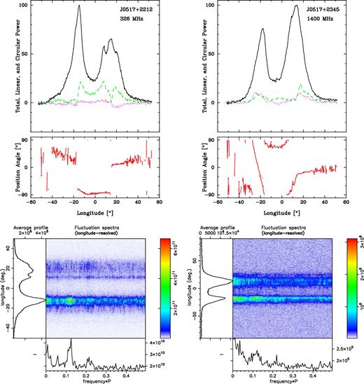
J0517+2212. It has a double-component profile at 1400 MHz, whereas its 327 MHz profile shows some structure in the second component. The polarization traverse shows little rotation at 327 MHz apart from the two 90° ‘jumps’, and the behaviour seems similar at 1400 MHz but less well resolved – perhaps because of the diminished fractional linear polarization. The fluctuation spectra show a peak around 0.12 cycles/period, suggesting an eight rotation-period modulation.
The increased structure at 1400 MHz, the overall pulse narrowing and the lack of PPA traverse suggest that β ∼ 0 and imply the outer conal beam geometry, as given in Table 5.
J0627+0706. It has a bright interpulse, separated from the main pulse by 177° (± 0|$_{.}^{\circ}$|27), as can be seen in Fig. 5. Because both features have structure, a more detailed interpretation is needed to assess how close to 180° they fall. However, given the narrowness of both features, it seems likely that they represent emission from the star's two poles, implying an orthogonal geometry, where α is close to 90°. PPA tracks give hints about the geometry only at 1400 MHz, and there is little to go on apart from a probable 90° ‘jump’ under the main pulse. The main pulse might have three components and the interpulse two. The fluctuation spectra are not displayed because they showed only flat ‘white’ fluctuations.
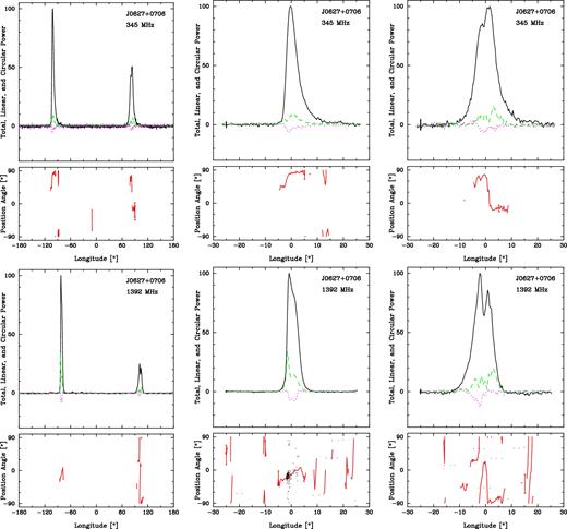
J0627+0706 327-MHz (upper row) and 1400-MHz (lower row) polarized profiles as in Fig. 3. The full periods displayed in the left-hand panels show the pulsar's main pulse and interpulse, and the centre panels and right-hand panels show them separately.
The pulse width at half-maximum widens from 327 to 1400 MHz, suggesting a core-single configuration where the conal emission is seen mainly at high frequencies. The polarization traverse is clearer at 1400 MHz, marked by prominent 90° modal ‘jumps’. It thus seems likely that β is small for the main pulse and perhaps larger for the interpulse, but that α is close to 90°, yielding the classifications and model values in Table 5. The emission heights given for both the main pulse and interpulse suggest that it is inner conal emission.
J0927+2345. It shows an interesting feature at 327 MHz approximately 180° away from the main pulse (Fig. 6) . This apparent interpulse is discernible only in the 327 MHz profile, and disappears in the 1400 MHz profile. Again, both profiles show so little linear polarization that a reliable PPA rate can be estimated for only a narrow longitude interval at 327 MHz. The main pulse appears to have three closely spaced features. The fluctuation spectra are not given for this pulsar because they showed no discernible features.
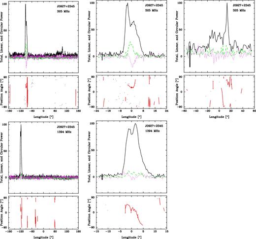
J0927+2345 as in Fig. 5. The pulsar's weak interpulse was not detected at the higher frequency separately.
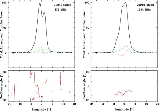
J0943+2253 polarized profiles as in Fig. 3.
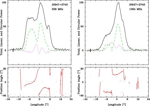
J0947+2740 polarized profiles as in Fig. 3.
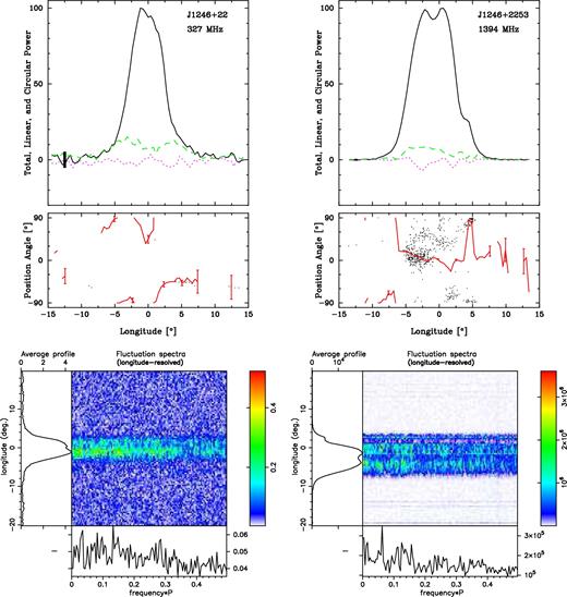
J1246+2253 polarized profiles and fluctuation spectra as in Fig. 3.
The half width broadens from 327 to 1400 MHz, suggesting a core single evolution where conal ‘outriders’ appear or become more prominent at high frequency. The polarization traverse is well defined only for a short interval at 1400 MHz, which provides a useful R value that leads to the geometric beam model in Table 5. If this profile were a triple, then the central component would be 2|$_{.}^{\circ}$|8 wide.
J0943+2253. It nulls, as shown in Fig. 1, but the fluctuation spectra show no quasi-periodic behaviour. There is slight linear polarization, and the PPA track shows what appears to be a 90° ‘jump’ within the narrow interval where it is clearly defined.
The average 327 MHz profile has two closely spaced components and perhaps an unresolved weak feature on its leading edge, suggesting a double or triple configuration. The 1400 MHz profile shows one main component, but there appears to be a bump on the leading edge, indicating an additional component. The linear polarization is slight and difficult to interpret at 327 MHz, but is slightly more pronounced at 1400 MHz. We measure a central PPA rate of at both frequencies in order to compute the geometric model parameters in Table 5, which suggest an inner-conal configuration.
J0947+2740. It shows three components at both frequencies, though the leading region may be more complex at the lower frequency, probably representing a core and closely spaced inner cone. At 1400 MHz, the conal components are weaker, and the PPA traverse is more complex. RVM behaviour and the slope of its polarization traverse could not be determined. This pulsar is also known to exhibit sporadic emission between intervals of weakness or nulls, as shown in Fig. 1. The fluctuation spectra (not shown) seem to hint at fluctuation power at periods longer than about three or four pulses.
The fact that the profile width increases with wavelength indicates an outer-conal configuration. Its PPA traverse seems interpretable as per the RVM model at 327 MHz, but its 1400 MHz traverse seems to be distorted by what may be a 90° ‘jump’ just prior to the profile centre. Its profile then seems to be a core/outer cone triple, and the quantitative beam geometry model is given in Table 5. The core width is estimated around 2|$_{.}^{\circ}$|65, which is much narrower than the central component of the profile (7|$_{.}^{\circ}$|92 at 327 MHz and 10.08° at 1400 MHz); this indicates that the magnetic axis is canted at 42°±2.7°.
J1246+2253. It has a single component at 327 MHz, which develops into a resolved triple form at 1400 MHz in what may be the characteristic core-single manner. The fractional linear polarization at both frequencies is low, so little can be discerned reliably from the PPA tracks. Also no clear features are seen in the fluctuation spectra as is often the case for core-single profiles.
The single profile at 327 MHz becoming triple at 1400 MHz strongly suggests a core-single configuration. Despite the low fractional linear polarization, the trailing positive traverse measured at 90° was used to compute the geometry in Table 5. The core width is calculated at 3|$_{.}^{\circ}$|55.
J1404+1159. It exhibits a narrow peak in its fluctuation spectra around 0.2 cycles/period, suggesting a modulation period P3 of some five rotation periods. A display of its individual pulses bears this out, and a plot of its emission folded at P3 shows that the modulation is highly regular. The PPA rate at the profile centre suggests an outside sightline traverse as is usual for conal single ‘drifters’ (see Fig. 10 ).
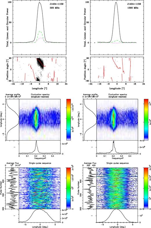
J1404+1159 polarized profiles and fluctuation spectrum as in Fig. 3. Additionally, a display showing the pulsar's accurately drifting subpulses is given at the bottom.
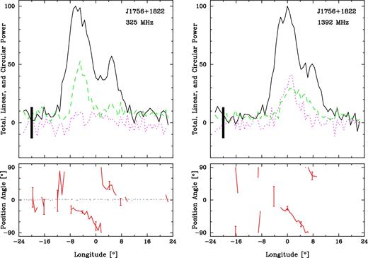
J1756+1822 polarized profiles as in Fig. 3.
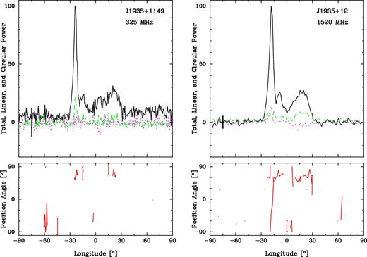
J1935+1159 polarized profiles as in Fig. 3.
The pulsar then appears to have a classic conal single profile. Both PPA tracks show a negative-going traverse with a central slope of −12 deg deg−1. Here, we also give short pulse sequences folded at the modulation period of some 0.2 rotation periods/cycle.
J1756+1822. It appears to have two profile components, and its profile broadens perceptibly with wavelength, suggesting a conal double configuration. Both frequency profiles have similar forms, with the longer wavelength profile somewhat broader in the usual pattern of the conal double class. The fractional linear profiles are low at both frequencies, but at 1400 MHz there seems to be a hint of a traverse through more than 90° across the profile. The fluctuation spectra are not shown as no features could be discerned.
J1935+1159. Its long nulls (see Fig. 1) make this pulsar difficult to observe sensitively, and neither clear profile structure nor polarization signature is seen at either frequency. Similarly, fluctuation spectra showed nothing useful.
It appears to be a four- or five-component pulsar even though only three components can be resolved, and appears to have the central PPA traverse and usual filled ‘boxy’ form which could hide additional components.
The emission heights, and the profile narrowing from 327 to 1400 MHz, indicate that this is an outer cone, which is filled with inner conal and/or core emission. For the geometric computations, we have estimated an unresolved central traverse of 10 ± 2 deg deg−1.
J2050+1259. It also exhibits frequent nulls, as shown in Fig. 1. However, its single profile at 1400 MHz broadens and bifurcates at 327 MHz in the usual conal double manner, and a steep PPA traverse is seen at the lower frequency. Here, we do see strong low-frequency features in the fluctuation spectra, indicative of modulation on a scale of 50 rotation periods or longer.
The profile has a single component at 1400 MHz and two closely spaced components at 327 MHz, as shown in Figs 1 and 13 . Its profile is broader at the lower frequency, and strong hints of a 90–180° PPA traverse are seen in both profiles, suggesting that this is a conal single profile with a small impact angle. Its beaming parameters are given in Table 5.
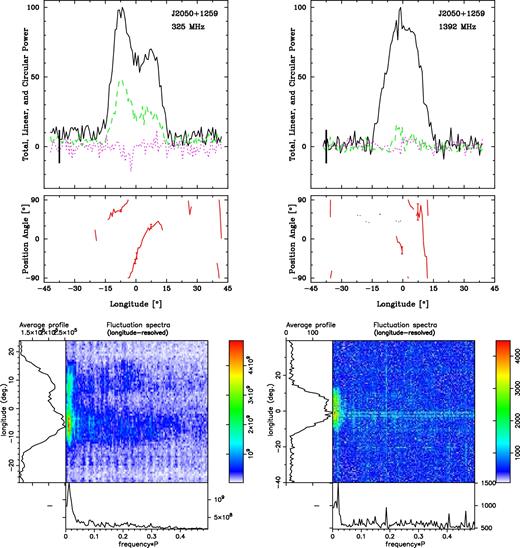
J2050+1259 polarized profiles and fluctuation spectra as in Fig. 3.
J2053+1718. Our observations do not provide much polarization information or fluctuation spectral information apart from it having a single profile at both frequencies. In the higher frequency observation, the time resolution was poor with only 232 samples across the rotation cycle. This pulsar has a wider profile at 1400 MHz than at 327 MHz; however, we hesitate to make conclusions about profile measurements due to the low quality of the observation. Despite this, its short 119-ms rotation period and single profile do suggest a core-single classification.
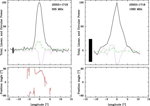
J2053+1718 polarized profiles as in Fig. 3.
4 ON THE ORIGIN OF PSR J2053+1718
In double-neutron-star systems, the first-born neutron star was recycled by accretion of mass from the progenitor of the second-formed neutron star. This accretion spun up the first formed NS to spin periods between 22 and 186 ms (for the known DNSs, likely faster right after they formed), and, by mechanisms that are not clearly understood, it induced a decrease in its magnetic field to values in the range 109 < B0 < 1010 G. Such pulsars spin down very slowly and therefore will stay in the active part of the P–|$\dot{P}$| diagram for much longer than non-recycled pulsars; this is the reason why we mostly see the recycled pulsars in these systems (the second-formed non-recycled pulsars are observed in two DNSs only). For a review, see Tauris et al. (2017).
Some isolated pulsars like PSR J2053+1718 are in the same area of the P–|$\dot{P}$| diagram as the recycled pulsars in DNSs, but have no companion to explain the recycling. The conventional explanation for their formation is that, like the recycled pulsars in DNSs, they were spun up by a massive stellar companion; the difference is that when the latter star goes supernova and forms a neutron star, the system unbinds, owing to the kick and mass-loss associated with the supernova (e.g. Belczynski et al. 2010). For this reason, they have been labelled ‘disrupted recycled pulsars’ (DRPs).
We should keep in mind the possibility of alternative origins for these pulsars: Some NSs observed in the centre of SNRs, despite being obviously young, have small B-fields and large characteristic ages similar to those of DRPs – these objects are known as central compact objects (CCOs; see e.g. Halpern & Gotthelf 2010). Therefore, one could expect that some DRPs formed as CCOs. However, Gotthelf et al. (2013) find, after an extensive study of DRPs in X-rays, that none appears to have thermal X-ray emission, implying that there is likely no relation between CCOs and DRPs. This results in a mystery: A substantial fraction of neutron stars appear to form as CCOs, which one might reasonably expect to form DRP-like radio pulsars, some of them with strong thermal X-ray emission, but these large numbers of DRPs (and ‘hot’ DRPs) are not observed. Either, for some unknown reason, they never develop radio emission, or their B-field increases significantly after birth, making them look more like normal pulsars. In any case, the results of Gotthelf et al. (2013) seem to exclude the possibility that DRPs such as PSR J2053+1718 formed from CCOs.
Any model that explains quantitatively the observed distribution of orbital eccentricities and spatial velocities of DNSs should also be able to explain the relative fraction of DRPs to DNSs and, furthermore, the velocity distribution of the two classes of objects. As already discussed by Belczynski et al. (2010), the relative number of DNSs and DRPs implies that the second SN kick must be, on average, significantly smaller than that observed for single pulsars. The evidence for this among DNSs has been growing in recent years and is now very strong (see comprehensive discussion in Tauris et al. 2017). It is therefore clear that more measurements of proper motions, spin periods, ages and B-fields of DRPs such as those presented here give us important clues for understanding the formation of DNS systems.
5 CONCLUSIONS
In this study, we have characterized a group of pulsars that had not been the target of any previous detailed studies. We determined timing solutions for them; most of them are normal, isolated pulsars. One of them, PSR J0627+0706, is relatively young (τc = 250 kyr) and is located near the Monoceros SNR; however, it is unlikely that the pulsar and that SNR originated in the same supernova event: We find that a nearby ‘radio-quiet’ pulsar recently discovered by the Fermi satellite, PSR J0633+0632, is located closer to the centre of the cluster and has a characteristic age that agrees better with the estimated age of the SNR.
We confirmed a candidate from a previous survey, PSR J2053+1718; subsequent timing shows that, despite being solitary, this object was recycled; it appears to be a member of a growing class of objects that appear to result from the disruption of double neutron stars at formation. We highlight that measurements of the characteristics of these objects (spin period, age, B-field, velocity) are important for understanding the formation of double neutron star systems.
As part of our characterization, we have also observed these pulsars polarimetrically with the Arecibo telescope at both 1400 and 327 MHz in an effort to explore their pulse-sequence properties and quantitative geometry. Three of them (PSRs J0943+2253, J1935+1159 and J2050+1259) have strong nulls and sporadic radio emission, several others exhibit interpulses (PSRs J0627+0706 and J0927+2345) and one shows regular drifting subpulses (J1404+1159). All these measurements will contribute to future, more global assessments of the emission properties of radio pulsars and studies of the NS population in the Galaxy.
Acknowledgements
Most of this work was made possible by support from the US National Science Foundation grant 09-68296 as well as National Aeronautics and Space Administration (NASA) Space Grants. One of us (JR) also thanks the Anton Pannekoek Astronomical Institute of the University of Amsterdam for their support. The Arecibo Observatory is operated by SRI International under a cooperative agreement with the US National Science Foundation, and in alliance with SRI, the Ana G. Méndez-Universidad Metropolitana and the Universities Space Research Association. This work made use of the NASA ADS astronomical data system. One of us (KS) thanks the US National Science Foundation for their support under the Physics Frontiers Center award number 1430284.
Footnotes
Standish E. M. 1998, ‘JPL Planetary and Lunar Ephemerides, DE405/LE405’, available at ftp://ssd.jpl.nasa.gov/pub/eph/planets/ioms/de405.iom.pdf
REFERENCES
