


Abstract
We investigate the lack of observed low-mass black hole binary systems at short periods(<4 h) by comparing the observed orbital period distribution of 17 confirmed low-mass black hole X-ray binaries (BHXBs) with their implied period distribution after correcting for the effects of extinction of the optical counterpart, absorption of the X-ray outburst and the probability of detecting a source in outburst. We also draw samples from two simple orbital period distributions and compare the simulated and observed orbital period distributions. We predict that there are >200 and <3000 binaries in the Galaxy with periods between 2 and 3 h, with an additional ≈600 objects between 3 and 10 h.
1 INTRODUCTION
Low-mass X-ray binaries (LMXBs) are binary systems consisting of a black hole (BH) or a neutron star primary and a low-mass main-sequence or an evolved companion star that is <1M⊙ (see e.g McClintock & Remillard 2006). Mass transfer occurs from the secondary to the primary via Roche lobe overflow. All of the dynamically confirmed low-mass black hole X-ray binaries (BHXBs) that have been observed are transient sources, spending most of the time in quiescence and occasionally going into outburst, when the source increases in X-ray luminosity by several orders of magnitude. The origin of the outbursts of transients is explained, at least in broad brush strokes, by the disc instability model (see reviews by Lasota 2001 and Maccarone 2014). The lack of persistent low-mass BHXBs may be, in part, due to selection effects. For example, the persistent source 4U 1957+11 is likely to be a BH (Wijnands, Miller & van der Klis 2002, Gomez, Mason & Robinson 2015), but dynamical confirmation has not yet been obtained because the accretion disc outshines the donor star in optical wavelengths; still there are few strong BH candidates in LMXBs that are persistently bright sources.
The orbital periods of these observed BHXBs vary from a few hours to several weeks (see Fig. 1). With the exception of GRS1915+105, all BH systems have an orbital period shorter than a week. However, there appears to be a lack of BHXBs at the shorter periods (<4 h) relative to theoretical predictions (Romani 1992, 1994; Portegies Zwart, Verbunt & Ergma 1997; Yungelson et al. 2006).
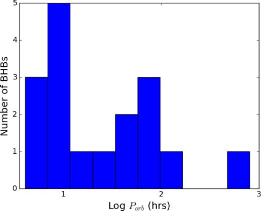
Histogram of the observed orbital period distribution of BHXBs. For a list of the properties of the binaries, see Table 1.
The peak X-ray luminosity of LMXBs during an outburst is directly proportional to the orbital period of the system (Shahbaz, Charles & King 1998; Portegies Zwart, Dewi & Maccarone 2004; Wu et al. 2010). This is a result of the binaries with a longer orbital period having a larger disc radius, and a larger radius to which the accretion disc is ionised by the central compact object.
When the mass accretion rates on to the primary are low and the local cooling time-scale becomes longer than the accretion time-scale, the accretion flow is radiatively inefficient. In this case, an advection dominated accretion flow (ADAF) can occur (Ichimaru 1977; Narayan & Yi 1995) and much of the kinetic energy in the accretion flow is advected on to the compact object. In the case of a BH primary, this energy is advected beyond the event horizon. In the case of a neutron star primary, however, the energy is radiated when the accretion flow impacts the stellar surface. This makes short-period BHXBs intrinsically fainter than their neutron star counterparts (Garcia et al. 2001).
It was shown by Knevitt et al. (2014) that the lack of short-period BH systems could be explained by a drop to a radiatively inefficient state at short periods due to the lower disc mass in these systems. In this case, the BHXBs have a lower peak luminosity in outburst, shorter outburst durations and lower X-ray duty cycles that result in the system being much harder to detect. They also calculated the detection probabilities of BHXBs in the Galaxy as a function of their orbital periods to show that this switch to a radiatively inefficient state renders these short-period systems undetectable at large distances.
In this paper, we investigate the impact of selection effects on the orbital period distribution of BHXBs by randomly distributing BHXBs across the Galaxy and calculating the fraction of sources that can be detected. We incorporate the switch to a radiatively inefficient state by assuming a gradual reduction in the radiative efficiency below a few percent of the Eddington luminosity as stated in Knevitt et al. (2014). In addition to this switch, we also take into account the effects of absorption of the X-ray flux to model the likelihood of the detection of the X-ray outburst.
LMXBs tend to be concentrated towards the plane of the Galaxy, where the extinction levels are the highest. Radial velocity measurements obtained when the system is in quiescence are required to get dynamical mass estimates of the BH candidate. In the case of short-period binaries which have less luminous companion stars than do longer period binaries, these high levels of extinction can result in the optical counterpart being too dim for these measurements. Thus, we have also included the probability of detecting the optical counterpart during quiescence in our calculations.
It is important to study and understand these effects because an accurate estimate of the population of BHXBs in the Galaxy can lead to more robust constraints on binary evolution models since the same physical process dominates the evolution of binaries irrespective of whether the primary is a white dwarf, neutron star or a BH. In this paper, we study the implied period distribution of BHXBs and estimate the total number of BHXBs in the Galaxy. In Section 2, we present our sample of BHXBs and the implied period distribution after correcting for various selection effects. In Section 3, we compare the implied period distribution to the period distribution drawn from two sample initial orbital period distributions and accounting for the effects of magnetic braking. This is followed by a discussion of our results and our conclusions.
2 DATA SET AND CORRECTION OF SELECTION EFFECTS
2.1 Galaxy model and data set
The data set consists of the 15 confirmed BH LMXBs and 2 strong candidate sources that have since been dynamically confirmed listed in McClintock & Remillard (2006). The sources and their properties are listed in Table 1. In order to determine what fraction of BHXBs are detected and dynamical mass measurements are obtained, 25 000 locations were randomly selected in the Galaxy. The random selection was weighted by stellar density, making it more likely for a binary to be located in the denser parts of the Galaxy. Each of the 17 BHXBs listed in Table 1 was then placed at each of the 25 000 locations to test for detectability. SWIFT J1753.5-0127 has not been included in our data set due to controversy over whether it really has been dynamically confirmed (Shaw et al. 2016).
Table of properties for the 17 BH LMXBs.
| Source name | Alternate name | Porb(h) | mVa | AV | Reference |
|---|---|---|---|---|---|
| GRO J0422+32 | V518 Per | 5.1 | 22.4 | 0.74 | Filippenko, Matheson & Ho (1995), Gelino & Harrison (2003) |
| A0620-00 | V616 Mon | 7.8 | 18.2 | 1.21 | Wu et al. (1976), Oke (1977), McClintock & Remillard (1986) |
| GRS 1009-45 | MM Vel | 6.8 | 21.7 | 0.62 | Filippenko et al. (1999), Masetti, Bianchini & della Valle (1997) |
| XTE J1118+480 | KV UMa | 4.1 | 19.0 | 0.06 | McClintock et al. (2001), Muno & Mauerhan (2006) |
| GRS 1124-684 | GU Mus | 10.4 | 20.5 | 0.9 | Remillard, McClintock & Bailyn (1992), Gelino, Harrison & McNamara (2001) |
| 4U 1543-475 | IL Lupi | 26.8 | 16.6 | 1.5 | Orosz et al. (1998) |
| XTE J1550-564 | V381 Nor | 37.0 | 22.0 | 4.75 | Orosz et al. (2002) |
| GRO J1655-40 | V1033 Sco | 62.9 | 17.3 | 4.03 | Bailyn et al. (1995), Orosz & Bailyn (1997) |
| GX 339-4 | V821 Ara | 42.1 | 19.2 | 3.4 | Kong et al. (2000), Hynes et al. (2003) |
| H 1705-250 | V22107 Oph | 12.5 | 21.5 | 1.2 | Yang et al. (2012), Remillard et al. (1996) |
| SAX J1819.3-2525 | V4641 Sgr | 67.6 | 13.7 | 0.9 | Orosz et al. (2001) |
| XTE J1859+226 | V406 Vul | 9.2 | 23.29 | 1.8 | Zurita et al. (2002) |
| GRS 1915+105 | V1487 Aql | 804.0 | –b | 19.6 | Greiner, Cuby & McCaughrean (2001), Chapuis & Corbel (2004) |
| GS 2000+251 | QZ Vul | 8.3 | 21.7 | 4.0 | Casares, Charles & Marsh (1995), Callanan & Charles (1991) |
| GS 2023+338 | V404 Cyg | 155.3 | 18.5 | 3.3 | Shahbaz et al. (1994), Casares et al. (1992) |
| XTE J1650-500 | – | 7.6 | 24.0 | 4.65 | Orosz et al. (2004), Garcia & Wilkes (2002), Augusteijn, Coe & Groot (2001) |
| GS 1354-64 | BW Cir | 61.1 | 21.5 | 3.1 | Casares et al. (2009), Kitamoto et al. (1990) |
aMagnitude in quiescence.
bFor calculating the detection fractions, the absolute magnitude of GRS 1915+105 was assumed to be MV = 0.
The modelling of the implied period distribution of the sources takes into account the probability of detecting the companion in quiescence, the probability of detecting an outburst with an all-sky monitor based on its location in the Galaxy, as well as the probability of the source having a detectable outburst based on the recurrence time and duration of the outburst. It is also worth mentioning that few of the BHXBs have repeated outbursts, and their recurrence times remain a key unknown. For more on the outburst recurrence times, see Section 2.4.
2.2 Extinction of optical counterpart
To determine the fraction of binaries for which the optical counterparts are too dim to obtain, radial velocity mass measurements due to the effects of extinction from the interstellar medium, the three-dimensional extinction model of Marshall et al. (2006) was used. The catalogue contains extinction profiles along over 64 000 lines of sight in the regions of |l| ≤ 100° and |b| ≤ 10° using 2MASS data. Linear interpolation of the data from the catalogue was used to determine the amount of extinction to each of the 25 000 locations determined as described in Section 2.1.
For the optical counterpart, a cut-off magnitude of V = 22 was selected. After accounting for extinction, sources along each line of sight brighter than this magnitude are considered to be bright enough for radial velocity measurements. The quiescent magnitudes used for the sources are listed in Table 1. Fig. 2 shows an example of the process of calculating the fraction of optical counterparts that are visible. The fraction of companion stars that are visible in the optical for each source is listed in Table 2.
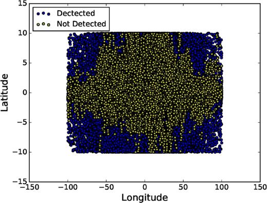
An example plot showing the detection of the optical counterpart for the source XTE J1150-564. The locations indicated by the blue filled circles are the locations where the optical counterpart can be observed. The yellow filled circles indicate locations where the optical counterpart cannot be detected due to high levels of extinction along that line of sight.
Detection fractions of BHXBs.
| Detection | Detection | Outburst | |
|---|---|---|---|
| Source name | fraction | fraction | detection |
| (X-rays) | (optical) | probability | |
| V518 Per | 0.0025 | 0.99 | 1.0 |
| V616 Mon | 0.025 | 1.0 | 0.38 |
| MM Vel | 0.0051 | 0.99 | 1.0 |
| KV UMa | 0.0085 | 0.0034 | 1.0 |
| GU Mus | 0.0078 | 1.0 | 0.38 |
| IL Lupi | 0.38 | 1.0 | 0.27 |
| V381 Nor | 0.22 | 1.0 | 0.21 |
| V1033 Sco | 0.38 | 1.0 | 0.27 |
| V821 Ara | 0.33 | 1.0 | 0.37 |
| V2107 Oph | 0.051 | 1.0 | 0.69 |
| V4641 Sgr | 0.44 | 1.0 | 0.13 |
| V406 Vul | 0.011 | 1.0 | 0.56 |
| V1487 Aql | 0.40 | 1.0 | 0.053 |
| QZ Vul | 0.072 | 1.0 | 0.43 |
| V404 Cyg | 0.34 | 1.0 | 0.11 |
| J1650-500 | 0.10 | 0.75 | 0.55 |
| BW Cir | 0.35 | 1.0 | 0.25 |
2.3 Detection of the X-ray outburst
To determine if the outburst would be visible, the recorded values of the peak fluxes seen from the sources were used to calculate the peak luminosities of the X-ray outburst. The outburst was considered to be detectable if the flux from the source exceeded 2.3 counts per second (corresponding to a 30 mCrab flux for Rossi X-Ray Timing Explorer All Sky Monitor, RXTE ASM) after accounting for the absorption column along that line of sight.
The conversion from X-ray flux counts per second was done using the NASA heasarc tool pimms. The values of hydrogen column density were obtained from Marshall et al. (2006), using NH = 1.79 × 10²¹AVcm−2 mag−1 (Predehl & Schmitt 1995). A standard photon index of Γ = 1.7 was assumed for all sources. The fraction of X-ray outbursts that can be detected for each source is listed in Table 2.
2.4 Probability of outburst detection
The value of density ρ = 10−8gcm−3 was chosen following King & Ritter (1998), where the density was shown to be independent of the radius, making it suitable for the wide range of orbital periods used.
The viscosity is taken to be ν = αhcsH = αhcs(H/R)Rd (Shakura & Sunyaev 1973; Pringle 1981) where cs is the speed of sound and H is the scaleheight of the disc. We have chosen a value of ν = 2.2 × 1014cm2s−1, as this produces a reduction in the radiative efficiency of BHXBs with an orbital period less than 5 h.
2.5 Implied orbital period distribution using observational data
Using the detection fractions shown in Table 2, the implied orbital period distribution was plotted. The results are shown in Fig. 3.
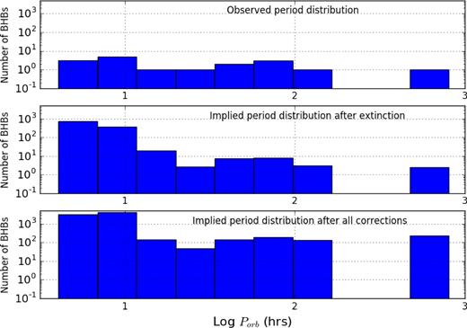
Top: histogram of the observed period distribution of BHXBs. Middle: distribution after accounting for extinction of optical counterpart. Bottom: distribution after accounting for extinction of optical counterpart, absorption of X-ray flux and the probability of detecting the X-ray outburst.
To compare the results with the distribution expected from theoretical models of magnetic braking, we fit a power-law slope to the results obtained after correcting for the selection effects detailed above. While the fitting of a constant cannot be excluded in a statistically significant manner, it is expected that the distribution follows a power law due to the physical processes dominating the evolution of the system (see equation 10). For this fitting, any sources with an orbital period greater than 10 h were excluded, since the evolution of these sources is likely to be dominated by expansion of the donor star, rather than by magnetic braking. The bin sizes used are unequal to ensure that none of the bins had a count of zero, and the error bars shown are Poissonian.
The fitting of the power law was done using xspec (Arnaud 1996). For the fitting, data from the observed BHXBs were converted to a spectrum file format using the flx2xsp routine in FTOOLS. Combining the optical detection fractions, the X-ray detection fractions and the probability of detecting the initial outburst gives the final fraction of the total BHXB population that can be observed. This final fraction was used as the corresponding response matrix for use with xspec. The results of the fit are shown in Fig. 4. We obtained a best-fitting value of 2.45 ± 1.3 for the plot assuming a 50 per cent mass-loss due to disc winds (i.e. N = 2 in equation 1). It was found that changing the amount of mass lost did not significantly alter the best-fitting value of the slope. It does, however, affect the normalization of the power law. These results are further discussed in Section 4. The large error bars on the fit are due to the small number of binaries with an orbital period less than 10 h.
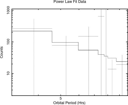
A power-law model fit to the predicted number of BH binaries in the Galaxy with an orbital period of less than 10 h.
3 MONTE CARLO SIMULATION
3.1 Generation of simulated sources
The age of each binary was selected randomly from a uniform distribution between 0 and 10 Gyr, and its current orbital period was determined using equation (10). A plot of the current orbital period of the binary as a function of its age is shown in Fig. 5. In these simulations, all the binaries were assumed to have a primary of mass equal to 8 M⊙. The companion mass was taken to be m2 = 0.1Porb(h) for Porb < 10 h, and m2 = 0.7 for Porb > 10 h. This way, the current orbital period distributions of the two samples were generated.
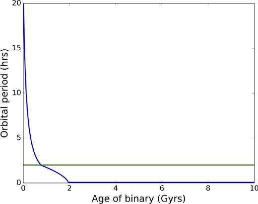
Plot of orbital period decay via magnetic braking and gravitational radiation for a system starting at an orbital period of 20 h. The green horizontal line indicates a 2 h orbital period, below which it is harder to observe the sources unless they are at a close distance.
3.2 Optical counterpart detection
A 50 per cent contribution of light from the accretion disc in quiescence was assumed and the locations of the binaries were selected randomly (weighted by stellar density). The effect of extinction was calculated as described in Section 2.2.
3.3 Probability of an X-ray outburst and its detection
The probability of detecting the X-ray outburst for these generated sources was calculated using the method detailed in Section 2.3. Once the detection fractions were calculated, a sample of 500 generated sources were randomly selected from each of the two distributions.
3.4 Implied orbital period distribution using simulated data
The best fits for the power-law index for the plots of number of detected sources versus the orbital period using the magnetic braking rate as shown in equation (10) are presented in Table 3. The plots of the best fits using a sample of 500 detected sources from each distribution can be seen in Fig. 6.

The best power-law fit obtained using xspec for the orbital period distribution of 500 randomly generated BH binaries with periods between 2 and 10 h. The binaries in the left-hand panel were drawn from an initial orbital period distribution that was logarithmically flat between 2 and 20 h and decay via magnetic braking. The binaries in the right-hand panel were drawn from an initial orbital period distribution where all the binaries start at a 20 h period and decay via magnetic braking.
Power-law fits to number of detected sources versus Porb.
| Distribution | No. of sources | Power-law index |
|---|---|---|
| Data | 7 | 2.45 ± 1.3 |
| Spikea | 500 | 1.60 ± 0.09 |
| Flatb | 500 | 2.38 ± 0.10 |
| Spike | 275 | 1.62 ± 0.12 |
| Flat | 275 | 2.38 ± 0.13 |
| Spike | 50 | 1.61 ± 0.31 |
| Flat | 50 | 2.36 ± 0.32 |
| Distribution | No. of sources | Power-law index |
|---|---|---|
| Data | 7 | 2.45 ± 1.3 |
| Spikea | 500 | 1.60 ± 0.09 |
| Flatb | 500 | 2.38 ± 0.10 |
| Spike | 275 | 1.62 ± 0.12 |
| Flat | 275 | 2.38 ± 0.13 |
| Spike | 50 | 1.61 ± 0.31 |
| Flat | 50 | 2.36 ± 0.32 |
aDrawn from an initial orbital period distribution where all the binaries start at a 20 h period.
bDrawn from an initial orbital period distribution that was logarithmically flat between 2 and 20 h.
3.5 Effect of mass transfer on the companion
The fit to the slope of the orbital period distribution plotted against the number of sources depends on the shape of the distribution that the sample is drawn from, as well as the relationship between the mass transfer rate and the orbital period of the system. In addition, due to the mass transfer that occurs during the lifetime of the donor star, the star can be expected to have a radius greater than the radius of an isolated main-sequence star of the same mass (King, Kolb & Burderi 1996). This bloating factor can also affect the slope of the plot, making it steeper.
4 DISCUSSION
By fitting the results of the implied period distribution from the observed binaries, a best-fitting value of 2.45 ± 1.3 was obtained for the plot assuming a 50 per cent mass-loss due to disc winds (i.e. N = 2 in equation 1). Changing the amount of mass lost to 66 per cent and 90 per cent did not significantly alter the best-fitting value of the slope.
From the results in Table 3, it would appear that the sample drawn from the flat orbital period distribution matches the data. The addition of the effect from the bloating of the companion star steepens the value of the slope by approximately 0.9, making the best-fitting value 3.28. However, due to the large error on the best fit to the slope of the observed data, the fit of the sample drawn from the spiked orbital period distribution cannot be excluded.
By integrating the implied period distribution to estimate the number of short-period BH binaries, we predict that approximately 600 BH binaries are present in the Galaxy with an orbital period between 3 and 10 h. Altering the amount of mass lost in winds to 66 per cent yields an estimate of ∼1100 binaries, and a loss of 90 per cent of the mass yields an estimate of ∼3700 binaries. It was estimated by Froning et al. (2011) that 90 per cent of the mass was lost due to disc wind and/or jets. This finding is based on estimating the mass transfer rate of the binary from the ultraviolet luminosity of the system under the assumption that the UV comes from the accretion stream impact spot on the outer disc in A0620-00, and then comparing with the duty cycle of the outburst, and is also supported by measurements of strong disc winds in the outbursts of X-ray binaries (e.g. Neilsen & Lee 2009). It has been alternatively suggested that the UV emission may come from closer to the BH in this system, in which case the inferred mass transfer rate would be much lower, and such strong disc winds would not be necessary (Hynes & Robinson 2012), although such a result would not explain the actual observations of strong disc winds in outburst. Thus, it is clear that a deeper understanding of the outburst duty cycle is needed to accurately estimate the total number of BH binaries in the Galaxy.
By extrapolating the fit down to 2 h, we predict that there are ∼200–3000 binaries with periods between 2 and 3 h. The range of the values are determined using the upper and lower limits of the power-law index estimate as shown in Table 3. Our estimate for the total number of BHXBs in the Galaxy is consistent with theoretical estimates of numbers between 102 and 104 obtained using population synthesis codes (Romani 1992, 1994; Portegies Zwart et al. 1997; Yungelson et al. 2006). However, Tetarenko et al. (2016) have detected a radio source in the direction of M15 that they have suggested is a BHXB in quiescence. If correct, it would imply a much larger population of quiescent BHXBs (2.6 × 10⁴–1.7 × 10⁸). While this could suggest a new channel of BH formation, it does not fit well with our predictions. It must also be emphasized that X-rays have not been detected from this source, and thus the estimate of a larger population must be treated with caution. While this discovery could be anomalous, it has been suggested that binaries lack outbursts at accretion rates lower than those predicted by magnetic braking. This could be the case for short-period binaries that exist in the period gap which, as discussed by Maccarone & Patruno (2013) may have low but non-zero accretion rates, as well as for the very long period systems suggested by Menou, Narayan & Lasota (1999). Thus, it is possible that there exists a hidden population of persistently quiescent BHXBs.
To estimate the number of binaries that would have to be detected and have dynamical mass estimates in order to determine which of the two distributions is closest to the true orbital period distribution, we ran the Monte Carlo simulation detailed in the previous section, drawing a different number of detectable sources each time. With a sample of 50 detected binaries, it is possible to distinguish between the two sample orbital period distributions at the 1σ level. A sample of approximately 275 binaries will be required to distinguish the two at the 3σ level. The next generation of X-ray missions such as LOFT (Feroci et al. 2012) and STROBE-X (Wilson-Hodge et al. 2017) is thus extremely important for identifying more of these short-period systems and understanding their underlying distribution.
The model used to predict the peak luminosities of the X-ray outburst produces a decrease in radiative efficiency at short orbital periods (Porb ≤ 5 h). However, the predicted luminosity for XTE J1118+480 is higher than the luminosity derived from the observed peak flux from the system. This was also noticed by Wu et al. (2010) who noted that this could be due to advection. If this is true in the case of all BHXBs with periods less than 5 h, then the detection of the X-ray outburst becomes the limiting factor, as opposed to the detection of the optical counterpart. In this case, the availability of sensitive all-sky monitors is the most effective tool in searching for this population of very faint, short-period BHXBs. This can already be seen by the large number of short-period BH candidates being detected by new, more sensitive wide field monitors. However, a number of these candidates cannot be confirmed due to the faintness of the companion in quiescence and an inability to obtain detailed spectroscopy for these objects. A possible solution to the problem in obtaining dynamical confirmation for short-period objects could be the relation proposed by Casares (2016) that allows the determination of the mass of the binary using H α emission lines, rather than absorption lines. Using this method could extend the search for short-period BHXBs to fainter limits, allowing us to confirm a larger fraction of candidate systems.
It is also worth noting that the addition of natal kicks to the simulation will result in an increase in the scaleheight of the BHXBs. See e.g. Jonker & Nelemans (2004) and Repetto & Nelemans (2015) for a discussion of the scaleheight distribution of BHXBs and corresponding evidence that most form with large natal kicks. This is likely to result in a larger fraction of binaries being detected due to the lower levels of extinction away from the Galactic plane. This can be seen by the detection of short-period systems at high galactic latitudes by MAXI (Yamaoka et al. 2012; Kuulkers et al. 2013) such as MAXI J1659-152 (Negoro et al. 2010; Kuulkers et al. 2013), MAXI J1836-194 (Negoro et al. 2011; Russell et al. 2014), MAXI J1305-704 (Sato et al. 2012; Shaw et al. 2017) and MAXI J1910-057 (Usui et al. 2012; Yoshii et al. 2014). The presence of natal kicks can also have an impact on the formation of BHXBs resulting from a wide binary interaction with a fly by star (Michaely & Perets 2016).
5 CONCLUSIONS
In this paper, we have derived the implied period distribution of low-mass BHXBs after correcting for the effects of extinction of the optical counterpart, absorption of the X-ray outburst and the probability of detecting a source in outburst. We have compared the power-law fit to the implied orbital period distribution to the distributions produced by drawing a sample from two simple orbital period distribution. Based on the results from the simulation, it is likely that the observed data arise from a flat orbital period distribution. However, due to the small number of observed sources, the possibility of an orbital period distribution arising from the decay of the orbit of a large orbital period (20 h) cannot be ruled out. With a sample of ∼275 detected sources, it would be possible to differentiate between the two distributions. Our simulation predicts ∼200–3000 binaries with periods between 2 and 3 h, and an additional ∼600 binaries between 3 and 10 h. This is consistent with numbers predicted using population synthesis models.
ACKNOWLEDGEMENTS
We would like to thank Chris Belczynski for ideas which motivated this paper, and Jorge Casares for useful discussions about finding more quiescent BHs and measuring their masses. We would also like to thank the anonymous referee for helpful and constructive comments.
REFERENCES
