


Abstract
We studied some statistical properties of the spatial point process displayed by GRBs of known redshift. To find ring-like point patterns we developed an algorithm and defined parameters to characterize the level of compactness and regularity of the rings found in this procedure. Applying this algorithm to the GRB sample we identified three more ring-like point patterns. Although, they had the same regularity but much less level of compactness than the original GRB ring. Assuming a stochastic independence of the angular and radial positions of the GRBs we obtained 1502 additional samples, altogether 542 222 data points, by bootstrapping the original one. None of these data points participated in rings having similar level of compactness and regularity as the original one. Using an appropriate kernel we estimated the joint probability density of the angular and radial variables of the GRBs. Performing MCMC simulations we obtained 1502 new samples, altogether 542 222 data points. Among these data points only three represented ring-like patterns having similar parameters as the original one. By defining a new statistical variable we tested the independence of the angular and radial variables of the GRBs. We concluded that despite the existence of local irregularities in the GRBs’ spatial distribution (e.g. the GGR) one cannot reject the Cosmological Principle, based on their spatial distribution as a whole. We pointed out the large-scale spatial pattern of the GRB activity does not necessarily reflects the large-scale distribution of the cosmic matter.
1 INTRODUCTION
In a recent paper, Balázs et al. (2015) reported the discovery of a giant GRB ring (GGR) consisting of nine objects in the 0.78 < z < 0.86 redshift range. The mean angular size of the feature is 36° corresponding to 1720 Mpc in a comoving reference frame. Voids surrounded by filaments are typical ingredients in the cosmic matter distribution. Their characteristic size, however, is at least an order of magnitude smaller than that of the ring (Frisch et al. 1995; Einasto et al. 1997; Suhhonenko et al. 2011; Aragon-Calvo & Szalay 2013).
GRBs are extremely energetic transients and distribute nearly uniformly on the sky (Briggs et al. 1996, and references therein). There are pieces of evidence, however, that the isotropy is valid only for the long GRBs (T90 > 10 s). Nevertheless, it is not the case at the short (T90 < 2 s) and intermediate (2 < T90 < 10 s) duration bursts (Balazs, Meszaros & Horvath 1998; Balázs et al. 1999; Cline, Matthey & Otwinowski 1999; Mészáros et al. 2000; Litvin et al. 2001; Magliocchetti, Ghirlanda & Celotti 2003; Cline et al. 2005; Tanvir et al. 2005; Vavrek et al. 2008; Tarnopolski 2017). Due to their immense intrinsic brightness they can be seen at very large cosmological distances and sofar they are the only observed objects sampling the matter distribution of the Universe as a whole, in particular testing the validity of the cosmological principle (CP, Ellis 1975).
The original intention of Balázs et al. was to test CP and the discovery of the GGR was only a byproduct. They pointed out that the fobs(l, b, z) joint probability distribution of the l, b angular coordinates and the z redshift can be factorized into g(l, b) × fintr(z), if CP is valid. Testing this hypothesis they found, unexpectedly the GGR.
Assuming that CP is valid there is an estimated transition scale of about 370 Mpc and the size of all the existing structures does not exceed it (Yadav, Bagla & Khandai 2010). Recently, large quasar groups (LQG) were reported significantly exceeding this size (Clowes et al. 2013). The largest structure (3 Gpc in diameter in a comoving reference frame) reported sofar is the enhancement of GRBs spatial density was reported by Horváth, Hakkila & Bagoly (2014) and Horváth et al. (2015).
Some concerns were raised, however, on these features as real physical objects. According to those concerns these features are too big to be causally connected. Einasto (2016) concluded that the LQGs found in the quasar space distribution can be reconstructed also from random samples making use a friend of friend algorithm. Based on the GRBs’ detected by the Swift satellite and have measured redshift, Ukwatta & Woźniak (2016) did not find any clustering and deviation from the CP.
Making use the Metropolis–Hastings algorithm and the spatial density distribution of the dark matter, as predicted by the MXXL simulation (Angulo et al. 2012), Balázs et al. made extensive studies to find giant ring-like features, without any success. They found that the largest scale of the deviation from the CP is 280 Mpc corresponding to the result of Park et al. (2012) in the Horizon2 simulation (Kim et al. 2011).
Assuming a linear relationship between the cosmic baryonic matter spatial and GRB number density, Balázs et al. calculated the mass of the giant ring and obtained a value of 1 × 10¹⁸ M⊙ which still represents an overdensity of a factor of 10 suggesting the ring mass is in the range of 1017–1018 M⊙ depending on the fraction of GRB progenitors in the stellar mass distribution.
Balázs et al. discussed also the possibility that the ring is a projection of a spherical shell. In this case to get the observed properties of the ring one have to assume that there was a period of |$2 \times 10^8 \, \mathrm{\text{yr}}$| of enchained GRB activity in the hosts along the shell.
The estimated mass of the ring significantly depends on the assumption of the GRB activity in their hosts displaying it. There are two extremes of this activity: linear relationship on the baryonic spatial density or the GRB frequency is higher along the ring but the matter density is the same as in the field. In the latter case, the ring-like feature has nothing to do with the spatial matter density and its existence does not violate the CP.
Regular features in GRBs’ spatial distribution, consequently, do not necessarily violate the homogeneity and isotropy of the total large-scale matter distribution, i.e. the CP. Large-scale spatial patterns in the star forming and in this case in GRB activity which do not follow necessarily the general spatial matter distribution cannot be ruled out.
Since Balázs et al. were looking for enhancements in the spatial number density of GRBs and not for regular patterns, we try in the following to find further ring-like features in the same data set. We repeat this procedure also on completely random samples in order to find their significance.
After attempting to get further regular features in the data, we test the independence of the angular and redshift distribution. We followed the way suggested by Balázs et al. and a direct one to obtain significance with an alternative method.
2 SEARCH FOR RING-LIKE FEATURES
We intended to make a comparison with the results of Balázs et al., therefore, we used in the following the same data set consisting of 361 GRBs.
2.1 Mathematical background
A possible general procedure is the following:
Find an appropriate statistic which minima results in the very nine points found by Balázs et al.,
determines the distribution of the statistic and get significance of the features found in this procedure.
Scrutinizing the feature of the nine points a possible statistic is the squared norm error of a circle in 3D which plane is orthogonal to the line between the centre of the circle and the origin (the observer). Actually the covering sphere of the nine points does not contain any other points. This property might be ensured by choosing first an aspirant point in space and next choosing the nine nearest points to the centre among data points.
2.2 Searching rings in real data
We made a run of the algorithm described in Section 2.1 at first on real data consisting of 361 GRBs. We sorted the objects according to the radial distance and formed groups of subsequent 17 GRBs step by step at each elements of the sample.
By running the algorithm we assigned a pattern consisting of nine GRBs to each objects in the sample. Running the algorithm results in an Rt thickness of the annulus embedding the nine points of the pattern. The local minima in Rt values may indicate ring-like patterns.
As one can infer from Fig. 1 the GGR is really lying in a local minimum of Rt. There are, however, other minima locating even deeper. We marked the three deepest ones with R1, R2 and R3 in the figure. The rings belonging to these minima are displayed in Fig. A1.
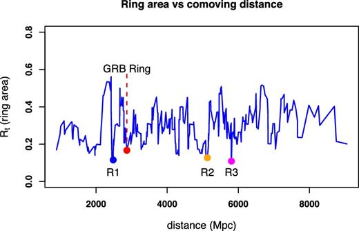
Dependence of the Rt ring area, computed in equation (3), on the comoving distance. The minima deeper than that of the GGR may represent ring-like features. The deepest three minima marked with coloured dots and labelled with R1, R2 and R3
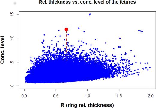
At the end of Section 2.1, we defined a parameter the level of concentration of a ring found in the procedure described in this section. In Fig. 2, we show the computed level of concentration of each pattern found by the ring-searching algorithm. One can see immediately that there is a marked difference between the real ring and those found by simply minimizing Rt.

Although, the R1, R2 and R3 objects show highly regular circular pattern they have much less level of concentration than the GGR. As Fig. 2 demonstrates it is quite an isolated object in this respect.
2.3 Searching rings in random samples
We pointed out in Section 2.2 the GGR is quite a unique object with respect to the level of concentration within the studied sample of 361 GRBs. In the following, we study the problem of getting such a unique pattern quite accidentally.
2.3.1 Searching in resampled data
Balázs et al. pointed out that in case of a valid CP the joint probability density of the angular and radial coordinates of the GRBs can be factorized, i.e. it can be written as a product of the radial and angular distribution. Supposing the validity of this property, a sample from the joint probability density of the angular and radial distributions remains statistically invariant if we reorder the radial distribution of GRBs, keeping the angular positions unchanged.
To perform this reordering we invoked the sample() procedure of the r statistical package.1 Making use 1502 times this procedure and combing the results with the unchanged angular coordinates we obtained 1502 independent samples of 361 GRBs. We made run the algorithm described in Section 2.1 in each of these samples, separately. The algorithm assigned a pattern of nine GRBs to each sample elements embedded in an annulus of a width as given in equation (3). Having Rt we get the relative width of the annulus dividing Rt by the internal radius of the annulus. We displayed this relative width versus the level of concentration of the feature in Fig. 3.
Result in searching rings in samples of resampled distances. Red dot marks the GGR. The figure consist of 542 222 dots obtained from 1502 simulations each consisting of 361−17+1 objects (see Section 2.1). All of them are representing a pattern of nine points. Note that there is no pattern having larger concentration and smaller relative thickness than those of the GGR.
As one can reveal from this figure none of the simulated features has higher level of concentration and smaller relative width of the embedding annulus than the GGR.
2.3.2 Searching in completely spatially random data
In Section 2.3.1, we reordered the distances of the GRBs but left their angular position unchanged. In this section, we simulate both the angular and radial distribution as well, assuming again the statistical independence of the angular and radial distribution, as we did it in Section 2.3.1.
The angular positions of the GRBs are distributed on a sphere. To do kernel smoothing one has to define the functional form and characterizing length of this procedure. For smoothing on spherically distributed data Hall, Watson & Cabrera (1987) suggest the functional form of et where t had the form of (wwi − 1)/h. In this expression, wwi is a scalar product of unit vectors pointing to an arbitrary and the ith sample points on the sphere, respectively and h is a smoothing length. Easy to see that w = wi gives t = 0 and et = 1.
For smoothing length we selected the largest value giving a pdf which was statistically still compatible with the original sample. For smoothing the radial data we used a kernel of a Gaussian form (see e.g. Bagoly et al. 2016). We showed the colour coded representation of the selection function in Fig. 4.
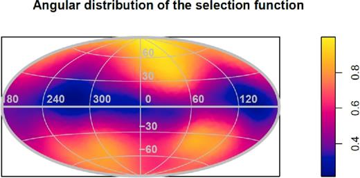
Colour coded representation of the selection function of equation (6) in Aitoff projection of Galactic coordinates. The dark strip along the equator is due to the Galactic foreground extinction.
Having in hand the pdf of both the angular and radial distributions we simulated random samples by making use Markov Chain Monte Carlo simulation (MCMC) realized by the Metropolis–Hastings algorithm (Metropolis et al. 1953; Hastings 1970) available in the metrop() procedure in the mcmc library of the r statistical package. We made run the MCMC simulations for getting angular and radial data, separately.
Performing this procedure 1502 times we obtained 1502 independent samples each getting a size of 361, altogether 542 222 objects in total. By making run the algorithm of Section 2.1 we assigned to all of these points a feature of nine objects, each having an embedding annulus of some level of concentration and relative thickness according to the final part of 2.1 and 2.3.1. The result is displayed in Fig. 5.
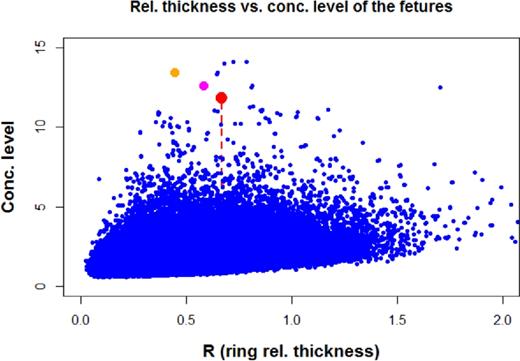
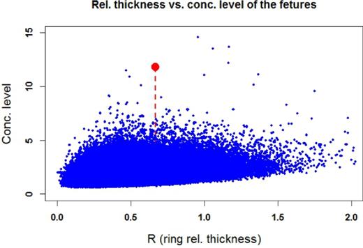
Scatter plot of relative thickness versus concentration level of patterns recognized in random data. Red dot marks the GGR. Orange and magenta dots indicate simulated patterns having larger level of concentration and less thick embedding annulus than those of the GGR. The number of simulations was 1502 each consisting of 361−17+1 objects (see Section 2.1) resulting in 518 190 dots in the figure. Note that there are only three points representing patterns having higher level of concentration and smaller relative thickness than that of the GGR.
One may infer from Fig. 5 that only three points are representing patterns of having higher level of concentration and smaller relative with of the embedding annulus than that of the GGR. This figure gives some hint for the probability of getting such a ring-like pattern fully accidentally (two of them are marked with orange and magenta colours and displayed in Fig. A2).
2.3.3 Searching in data of uniform angular distribution
We showed in Sections 2.3.1 and 2.3.2 that a GRB ring having the same size and regularity than GGR is a low probability phenomenon to get it only by chance. This conclusion was based, however, on the resampled data and those obtained from the MCMC simulation. In both cases the original angular distribution of the objects were seriously biased by selection effects as the exposure function of detecting GRBs, the availability of the necessary telescope time for measuring redshift and the Galactic foreground extinction.
One may have concerns, therefore, that these selection effects may seriously modify also the probabilities of getting ring-like features, such as the GGR. Namely, due to the angular irregularities of the selection effects an existing ring-like feature can be recorded by parts only, and not detected by the algorithm described in Section 2.1.
In Section 1, we already mentioned that the long GRBs distribute on the sky nearly uniformally. Most of the GRBs having measured redshift belong to this group. Accepting that the true angular distribution of GRBs is uniform the f (x) surface density defined in equation (6) represent the actual selection function inserted by the observations on the true angular distribution. Accepting this assumption one may estimate the size of the unbiased sample from which the observed size was obtained.
Proceeding in this way we estimated the size of the true sample of uniform angular distribution resulted in the observed one by applying the f (x) selection function. We obtained a size of about 700 for the unbiased sample, in this way. We simulated a sample with this size of uniform angular distribution. The distribution of the GRB distances was obtained in the similar way as in Section 2.3.2.
We made run the algorithm of Section 2.1 on the sample obtained in this way and repeated this procedure 1503 times, resulting 1052.100 objects in total. The results is displayed in Fig. 6. It clearly demonstrates that no simulated features exists with higher level of concentration and regularity than GGR.
Result in searching rings in samples of uniform angular distribution. Red dot marks the GGR.The figure consist of 1029.555 dots obtained from 1503 simulations each consisting of 700−17+1 objects (see Section 2.1). Each represents a pattern of nine points. Note that there is no pattern having larger concentration and smaller relative thickness than those of the GGR.
In conclusion, getting a ring-like feature, similar to GGR, has a very low probability to find it purely accidentally, even in a sample of unbiased uniform distribution.
3 TESTING INDEPENDENCE
The original intention of Balázs et al. was to test the validity of CP making use a sample of GRBs with known redshifts. They pointed out that in case of a valid CP the joint pdf of the observed angular and radial coordinates can be factorized into an angular and radial part. The discovery of the GGR was only a byproduct.
If the joint pdf can be factorized into an angular and radial part it means the angular and radial distributions of GRBs are stochastically independent.
In simulating the joint angular and spatial distribution of GRBs we assumed the stochastic independence between these distributions and, consequently, the validity of factoring the joint pdf into a radial and angular part. In the following we test the independence of angular and radial distribution of GRBs, directly.
Assuming the validity of the null hypothesis, i.e. the angular and radial distributions are independent we can get the distribution of the V variable in equation (9) using the samples obtained from the simulations outlined in Sections 2.3.1 and 2.3.2.
The distributions of V for the resampled and the completely random sample is given in Fig. 7 where the red vertical dashed line indicates the value of the real GRB sample. One can infer from comparing the histograms in the upper and lower panel of the figure that the distributions of V in the resampled and the completely random sample are not fully identical.
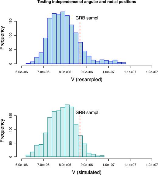
Distribution of the V variable defined in equation (9). The upper panel shows the distribution obtained from the resampled data and the lower one from that of the completely random case. The red vertical dashed line indicates the V value of the real GRB sample. The position of the real sample in the figures reveal that it does not contradicts to the null hypothesis, i.e. the angular and radial distribution of GRBs are statistically independent.
Already at the first glance, in Fig. 7 the maximum of the upper histogram is a little bit shifted with respect to the lower one. Furthermore, the upper histogram has a wing towards higher V values which is absent in the lower panel. Comparing the two distributions by means of the Kolmogorov–Smirnov (KS) test gives a probability of p = 5.48 × 10⁻¹¹ for the validity of the null hypothesis, i.e. the upper and lower histograms of Fig. 7 come from the same parent distribution.
There is a trivial explanation for the highly significant difference between the V distributions obtained from the resampled and the completely random data. We may assume they have different pdf, although both can be factorized into an angular and a radial part. Nevertheless, the random pdf was obtained by a kernel procedure based on the true GRB data and keeping control on the compatibility between the simulated and the original distribution. Therefore, this trivial explanation can be excluded.
The different approach in obtaining the samples can be the reason for the stochastic difference between the resampled and the random case. In getting the resampled data both the angular and radial positions are identical with those of the original GRB sample. The procedure changed only the order of the data. In the random case, however, any position is eligible assuming we are still compatible with the parent distribution obtained by the kernel smoothing. If the original sample has some internal order which is invariant against reordering it is still present after resampling unlike to the random case.
It is easy to see that a clustering in the spatial distribution of the objects results in systematically smaller values in ϱ(κi) − ϱ(i) differences in equation (9) and the opposite is true in the case of voids. The presence of voids is quite characteristic in the large-scale distribution of cosmic matter (Einasto, Joeveer & Saar 1980; Zeldovich, Einasto & Shandarin 1982; Icke 1984; Icke & van de Weygaert 1991; Einasto et al. 1997; Gott et al. 2005; Einasto et al. 2011, 2014). The resampling of the GRB data does not necessary destroy the void structure and this may cause the wing of the larger V values in the upper panel of Fig. 7.
In both cases, however, the factorization of the joint angular and radial distribution is valid so the independence is true at this statistical level.
Therefore, our result indicates that according to the distribution of the V variable there is no significant deviation from independence based neither on the resampled nor on the complete random samples.
4 DISCUSSION
Testing the validity of CP is a basic problem of the observational cosmology. Large-scale deviation from the homogeneous isotropic distribution of the cosmic matter casts a serious doubt on the applicability of the Friedman-Lemaitre-Robertson-Walker model for the Universe as a whole.
Until now the GRBs are the only objects sampling the space distribution in the Universal matter as a whole. It is a problem, however, that the number of GRBs with known redshift, i.e. with spatial position, is very low (a few hundred, but steadily increasing). Furthermore, it is also a problem whether their spatial distribution represent a bias free sample of the global distribution of cosmic matter including dark energy and matter.
GRBs are not physically similar objects. Traditionally, they were divided into two basic classes: the short (T90 < 2 s and long (T90 > 2 s) ones. There are some indications for an intermediate duration group between them (Mukherjee et al. 1998; Horváth 1998, 2002, 2009; Horváth et al. 2006, 2008; Huja, Mészáros & Řípa 2009; Horváth et al. 2010; de Ugarte Postigo et al. 2011; Tsutsui & Shigeyama 2014; Zitouni et al. 2015; Horváth & Tóth 2016). The vast majority of GRBs having measured redshift belongs to the long group. Observational pieces of evidence (Mészáros et al. 2006; Chary, Berger & Cowie 2007; Yüksel et al. 2008; Kistler et al. 2009; Wang & Dai 2009; Ishida, de Souza & Ferrara 2011; Wei et al. 2014) connect the long GRBs to the star-forming activity in the underlying host galaxy and theoretical arguments relate them to the collapse of high-mass (at least 25–30 M⊙) stars into a rotating black hole (Woosley & Bloom 2006, and the references therein).
4.1 GRBs and large-scale pattern of star-forming rate
Because of the tight relationship of the GRBs, having measured redshift, to the high-mass star formation the observed spatial distribution of these objects reflects some large-scale/temporal pattern of star-forming activity and not necessarily the distribution of the cosmic matter as a whole.
As we pointed out above the redshift/time distribution of GRB activity versus the time dependence of cosmic star formation rate are closely related. The large-scale spatial distribution of the star formation rate, however, is an open issue.
The large-scale inhomogeneity in the GRBs’ spatial distribution may have a close relationship with large-scale spatial variation of the star formation rate but not with the cosmic matter distribution. Based on the Millennium simulation (Springel et al. 2005), Balázs et al. (2015) presented pieces of evidence that the large-scale spatial distribution of the normal galaxies and those having high star formation rate are different.
Estimating the total stellar mass associated with the GGR Balázs et al. considered two extremes:
The general spatial stellar mass density is the same in the field and in the rings region and only the star formation and consequently the GRB formation rate is higher here.
There is a strict proportionality between the stellar mass density and the number density of the progenitors.
For both estimates, one needs to know the local stellar density. Proceeding in these ways they got a range of the mass of the ring of 1017–1018 M⊙.
Alternatively Balázs et al. discuss the possibility that the ring is actually a projection of a shell. The observed properties is obtained if the ring is only a temporary configuration with an estimated lifetime of 2 × 10⁸ yr. The estimated mass of the whole structure is approximately an order of magnitude greater: i.e. 1018–1019 M⊙.
The masses in the above estimations consists of stars only. In the canonical Λ cold dark matter model, however, it is only a small fraction of the total one. Unless, the GGR was resulted in an enhancement of star-forming activity in the host galaxies and the mass density inside is the same as in the environment it may represent also a significant excess of the general matter density
The large amount of excess gravitating matter would have an imprint on the cosmic microwave background (CMB, Cruz et al. 2008; Génova-Santos et al. 2008; Das & Spergel 2009; Masina & Notari 2009; Padilla-Torres et al. 2009; Bremer et al. 2010; Granett, Szapudi & Neyrinck 2010; Solov'ev & Verkhodanov 2010; Chingangbam et al. 2012; Fernández-Cobos et al. 2013; Kovács & Granett 2015; Kovács & García-Bellido 2016) due to the integrated Sachs–Wolfe effect (Sachs & Wolfe 1967). A shell would have a ring on the CMB. Since no such effect was observed in our case the ring may be a large-scale pattern of increased star-forming activity and not necessarily a density enhancement.
4.2 Cosmic rings and global topology of the Universe
No matter how the GRBs’ large-scale spatial distribution relates to the total mass density their coordinates represent a stochastic point process in the comoving reference frame, from strictly statistical point of view. We followed this approach in this work, independently of the real physical processes ending up in their appearance as cosmic transients.
Treating the space distribution of GRBs strictly as a spatial stochastic point process, regardless of its genesis, we demonstrated in Sections 2.2 and 2.3 that a ring-like feature, having the same level of concentration and regularity, is a rare event getting it purely by chance. Therefore, it is worth studying physical processes resulting in ring-like structures.
Cosmological N-body simulations (Fall 1978; Aarseth & Fall 1980; Efstathiou et al. 1985; Bertschinger & Gelb 1991; Bagla & Padmanabhan 1997; Bagla 2005; Springel et al. 2005; Kim et al. 2011; Angulo et al. 2012; Joyce & Labini 2013; Valkenburg & Hu 2015; Garrison et al. 2016) attempted to reproduce the large-scale spatial distribution of dark matter. The simulations resulted in a system of strings and voids (displaying rings in 2D projections) having the maximal size of about 150 Mpc, i.e. an order of magnitude less size than the GGR The largest structure obtained in the s Horizon2 simulation (Kim et al. 2011) had a size of about 250 Mpc (Park et al. 2012). The number of the existing GRBs with known redshift is more than an order of magnitude less to that would be necessary to reveal this structure (Balázs et al. 2015).
The characteristics of the cosmic web resulted in these N-body simulations depend on the choice of the initial conditions. In this context assuming the homogeneity of the initial conditions seems to be consistent with the observable angular isotropy of the CMB. Although, the large-scale isotropy of the CMB is widely accepted (Planck Collaboration XXIII 2014; Planck Collaboration XVI 2016) there are attempts to find large-scale deviations from it (Hajian & Souradeep 2003; Basak, Hajian & Souradeep 2006; Souradeep, Hajian & Basak 2006; Lew 2008; Aich & Souradeep 2010; Peiris & Smith 2010; Zhang 2012; Mukherjee, De & Souradeep 2014).
Solutions of Einstein's equation specify only the local properties of the cosmological space. It does not constrain, however, its global topology. Conventionally, one assumes that the space is simply connected and the infinity can be a reality. Nevertheless, in a multiply connected case the physical world can be finite and the infinity is only a pretence (Paál 1971).
Obviously, RLSS can be substituted by the radius of any sphere dedicated by some physical phenomenon, i.e. by GRBs, in equation (10). Of course, the size of the real world has to be less than this radius. The celestial position of the ring obtained in this way is given by the global topology of the cosmic space and not necessarily populated by any GRB events. Even if the GRBs would populate the real space completely randomly the probability to find an evens along the ring is higher.
There were many attempts to identify ring-like patterns in the CMB (Mota, Rebouças & Tavakol 2008, 2010; Moss, Scott & Zibin 2011; Mota, Rebouças & Tavakol 2011; Wehus & Eriksen 2011; Gomero, Mota & Rebouças 2016) the results, however, were not conclusive. Kovetz, Ben-David & Itzhaki (2010) found a unique direction in the CMB sky around which giant rings have an anomalous mean temperature profile. The score of the ring is close to the direction of the cosmic bulk flow (Kashlinsky & Atrio-Barandela 2000; Kashlinsky et al. 2008, 2009, 2010, 2013; Kashlinsky, Atrio-Barandela & Ebeling 2011). They estimated the significance of the giant rings at the 3σ level. The recent detailed analysis of the Planck data (Planck Collaboration XVI 2016), however, concluded: there is no sign for a multiple connected topology in the CMB data.
4.3 Cosmic rings and large-scale cosmological perturbations
Large-scale deviations of the cosmic matter density from the homogeneous and isotropic case are accompanied with inhomogeneities in the gravitational space might have footprints on the CMB. The opposite is not necessarily true. Inhomogeneity in the CMB not necessarily means gravitational irregularities. A reason for it could be the improper elimination of the Galactic foreground. The effect of the Galactic foreground is frequency dependent but that of the gravitational irregularities is achromatic.
In Section 4.1, we have already mentioned that a mass anomaly of the size of the GGR may result in a spot in the CMB, due to the integrated Sachs–Wolfe effect. Since there is no such a significant signal the statistical properties of the CMB would make an upper limit for the density of this concentration.
Solving this problem Eingorn (2016) found a λ characteristic length of Φ with a current value of λ0 ≈ 3700 Mpc. It is worth noting that this range and largest known cosmic structures (Clowes et al. 2013; Horváth et al. 2014; Balázs et al. 2015) are of the same order and their sizes essentially exceed the previously reported epoch-independent scale of homogeneity ∼370 Mpc (Yadav et al. 2010).
We have already mentioned that a spatial enhancement in the GRB activity does not necessarily mean the same in the underlying general matter density. The GRB activity directly relates to the formation rate of the high-mass stars. Based on the Millennium simulation (Springel et al. 2005) Balázs et al. (2015) demonstrated: the spatial distribution of the galaxies does not follow that of having high star formation rate, in general.
Collision between galaxies is an important source of the enhanced star formation activity (Sanders & Mirabel 1996, and the references therein). However, this does not mean that interacting galaxies are necessarily starbursts. Triggering depends on many factors, e.g. the specific merging geometry and the progenitor galaxies’ properties (Mihos & Hernquist 1996; Springel 2000; Springel & Hernquist 2005; Cox et al. 2006, 2008; Di Matteo et al. 2007, 2008; Torrey et al. 2012; Moreno et al. 2015). The frequency of collisions depends on the square of the number density of the objects participating in collisions.
Let us suppose a δν first order perturbation in the ν0 spatial number density, ν = ν0 + δν, the frequency of collisions proportional to |$\nu ^2 \approx \nu _0^2+2\delta \nu$|. Consequently, the amplitude of the increase of the collision frequency is higher with a factor of 2 than that of the δν number density enhancement. Therefore, it may happen that one finds anomalies in the GRBs’ spatial distribution at some level of significance which is not shown in other cosmic objects.
In conclusion, density perturbations having the characteristic size of the GGR may exist. The identification its imprint in the spatial distribution of the observed objects needs a statistically significant signal due to their spatial density. As to the GRBs’ spatial distribution the amplitude of this signal is at least a factor of 2 higher in case if the high star-forming activity is given by the galaxy collisions. Consequently, anomalies in GRB distribution can exist which are not necessarily shown in other cosmic objects. Further detailed observations are necessary to get a satisfactory solution of this problem.
4.4 GRBs’ spatial distribution and validity of CP
Even if the spatial density of the baryonic matter is constant in the comoving reference frame the formation of cosmic objects is a long lasting complex procedure and their spatial distribution reflects the history of their formation. As a consequence the spatial homogeneity was lost. It is also true for the spatial distribution of GRBs. In contrast, the isotropy is still hold.
In the case of isotropy the ν spatial number density depends only on the distance of the object to the observer but not on the angular coordinates. Since the sum of Poissonian distributions is also Poissonian and the column density replaces ν and the area the V volume.
In the case of spatial isotropy the angular distribution of GRBs would be uniform, if there were no observational selection effects. It can be demonstrated that correcting to the effect of exposure function the angular distribution of long GRBs (T90 > 2 s) is isotropic but it is not the case of the short (T90 < 2 s) and intermediate (2 < T90 < 10 s) ones (see the references listed in Section 1). The reason for this result is the much larger volume sampled by the observed long bursts than the short ones.
Only a small fraction (a few hundred) of the known GRBs have measured redshifts, i.e. known distances. Besides the exposure function the GRB distribution of known redshift suffers from the selection effect due to the availability of the necessary telescope time and the extinction of the Galactic foreground.
In the case of isotropy the w angular position of an object is statistically independent of the r distance. Consequently, the joint probability density f(w, r) of the angular position and radial distance can be factorized into an g(w) angular and h(r) radial part, i.e. f(w, r) = g(w)h(r) (Balázs et al. 2015). They also pointed out the selection effects due to the telescope time and Galactic foreground extinction does not influence this factorization. The factorization means a stochastic independence of the angular and radial positions.
The stochastic independence is a necessary, but not sufficient, requirement of the validity of the CP. We tested this independence in Section 3 and concluded that the GRB actual sample of known redshift did not contradict to assuming stochastic independence between the angular and radial positions.
This conclusion seems to contradict to the existence of the GGR having a characteristic size of 1720 Mpc significantly larger than the 370 Mpc transition scale (Yadav et al. 2010) to the valid CP. The GGR, however, consists of only nine objects. According to Section 2.3.1 resampling the original GRB sample 1502 times did not reveal ring-like features having at least the same level of concentration and regularity. However, shown in Section 3 the whole sample was still consistent with assuming a stochastic independence between the angular and radial coordinates.
We may conclude, the local anomalies (e.g. the existence of the GGR) in the sample of the GRBs with known spatial position does not allow to reject the CP with a sufficiently high level of significance. Even if they did, GRBs represent only a tiny fraction of the cosmic matter density. We cannot reject CP with a high level of certainty until it is supported by a notable fraction of the total cosmic matter density. Quite recently a study of the general distribution of the cosmic dark matter revealed it distributes much more evenly than previously was thought (Hildebrandt et al. 2017).
5 SUMMARY AND CONCLUSION
We studied some statistical properties of a stochastic point process defined by the positions of GRBs with known redshift in the comoving reference frame. The sample studied was identical with that used by Balázs et al. (2015) for discovering the GGR.
We developed an algorithm, described in Section 2.1, for finding ring-like point patterns in the sample. Since the GGR consists of nine bursts, concretely we were looking rings of this size. This choice excludes ring with less element but find all consisting of at least nine elements. We defined a concentration level and a measure of regularity to get a similar pattern as the giant ring.
Applying this procedure we identified additional three rings having better level of regularity, displayed in Figs 1 and 2. One may infer from these figures, however, the additional three rings found in this procedure have better level of regularity but they are far less concentrated than GGR.
Assuming a stochastic independence between the angular and the radial coordinates we generated 1502 bootstrapped samples from that used by Balázs et al. (2015), making use the sample() procedure of the r statistical package. The bootstrapped samples consisted of altogether 542 222 data points but none of them participated in a ring-like pattern of similar concentration and regularity than that of the original GGR.
Using an appropriate kernel we estimated the angular and radial probability density functions. Assuming again the independence of the angular and radial coordinates we generated random samples. We made MCMC realized by the Metropolis–Hastings algorithm available in the metrop() procedure in the mcmc library of the r statistical package.
Similarly, as we did in the case of the bootstrapped sample we simulated 1502 samples consisting of all together 542 222 data points. As one can infer from Fig. 5 out of these points only three represented ring-like point patterns having at least the concentration level and regularity as of the GGR.
We studied the effect of the selection bias on the probability of getting a GGR like feature purely accidentally. This selection bias comes into being through the superposition of the exposure function of detecting GRBs, the availability of the necessary optical telescope time and the Galactic foreground extinction. We simulated 1503 samples each having a size of 700, 1052.100 objects in total. (This is the size which is resulted in the observed sample after applying the selection bias.) We concluded, the combined effect of this selection bias does not change significantly the probability of getting a GGR like feature only by chance.
In the simulations given in Sections 2.3.1, 2.3.2 and 2.3.3, we assumed the stochastic independence of the w angular and r radial coordinates. In Section 3, we defined a V test variable measuring the level of independence. Based on the distributions obtained from the bootstrapped and MCMC simulations we obtained an empirical distribution of the V variable.
Since the long GRBs relate to the high-mass star formation their spatial distribution represents a large-scale footprint of this process. We pointed out in Section 4.1 the large-scale pattern of GRBs’ spatial distribution does not necessarily follow that of the total mass in the Universe.
Ring-like features in the distributions of some special cosmic objects may indicate a multiply connected global topology of the Universe. Based on the latest analysis of the Plank satellites data, however, one can exclude such an explanation of the GGR.
A galaxy–galaxy collision is one of the major sources of the enhanced star-forming activity and consequently of the GRB rate. The number of collisions is proportional to the square of the number density of galaxies. In the case of small amplitude perturbations it gives a factor of 2 higher statistical signal in the spatial number density of GRBs than the underlying matter density in general. One needs further observations to uncover the true relationship between the spatial number density of GRBs and that of the underlying matter in general.
Comparing the simulated distributions with the V value of the real GRB sample (see Fig. 7), we demonstrated that it did not contradict to assume stochastic independence between the w angular and r radial coordinates also in the real case. This result also implies that as a whole the GRB sample of known redshifts does not contradict to the CP.
Acknowledgements
This work was supported by the OTKA grant NN 111016. We are grateful to Dr. Jon Hakkila, the referee, for his advises and recommendations. The authors are indebted to N.M Arató, Z. Bagoly, I. Horváth, I.I. Rácz and L.V. Tóth for valuable comments and suggestions.
REFERENCES
APPENDIX A: EXAMPLES OF RING-LIKE PATTERNS

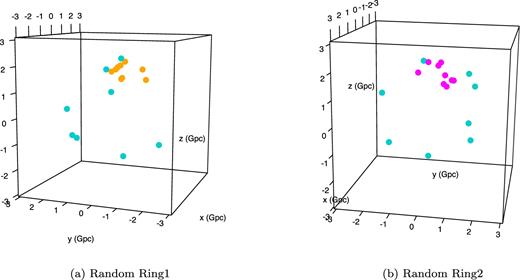
3D plot of rings obtained from random samples. (The colours of the ring patterns correspond to those applied in Fig. 5.)
