The relationship between galaxy and dark matter halo size from z ∼ 3 to the present

Somerville, Rachel S.; Behroozi, Peter; Pandya, Viraj; Dekel, Avishai; Faber, S. M.; Fontana, Adriano; Koekemoer, Anton M.; Koo, David C.; Pérez-González, P. G.; Primack, Joel R.; Santini, Paola; Taylor, Edward N.; van der Wel, Arjen

doi:10.1093/mnras/stx2040

Abstract

We explore empirical constraints on the statistical relationship between the radial size of galaxies and the radius of their host dark matter haloes from z ∼ 0.1–3 using the Galaxy And Mass Assembly (GAMA) and Cosmic Assembly Near Infrared Deep Extragalactic Legacy Survey (CANDELS) surveys. We map dark matter halo mass to galaxy stellar mass using relationships from abundance matching, applied to the Bolshoi–Planck dissipationless N-body simulation. We define SRHR ≡ r_e/R_h as the ratio of galaxy radius to halo virial radius, and SRHRλ ≡ r_e/(λR_h) as the ratio of galaxy radius to halo spin parameter times halo radius. At z ∼ 0.1, we find an average value of SRHR ≃ 0.018 and SRHRλ ≃ 0.5 with very little dependence on stellar mass. Stellar radius–halo radius (SRHR) and SRHRλ have a weak dependence on cosmic time since z ∼ 3. SRHR shows a mild decrease over cosmic time for low-mass galaxies, but increases slightly or does not evolve for more massive galaxies. We find hints that at high redshift (z ∼ 2–3), SRHRλ is lower for more massive galaxies, while it shows no significant dependence on stellar mass at z ≲ 0.5. We find that for both the GAMA and CANDELS samples, at all redshifts from z ∼ 0.1–3, the observed conditional size distribution in stellar mass bins is remarkably similar to the conditional distribution of λR_h. We discuss the physical interpretation and implications of these results.

galaxies: evolution, galaxies: formation, galaxies: high-redshift, galaxies: structure

1 INTRODUCTION

Our standard modern paradigm of galaxy formation posits that galaxies form within dark matter haloes, and much recent work has focused on empirically relating the observable properties of galaxies with those of their host haloes. While there are many ways to approach this problem, a commonly used approach to constrain the relationship between the stellar mass (or luminosity) of galaxies and the mass of their host dark matter haloes (the SMHM relation) is (sub-)halo abundance matching (SHAM; Conroy, Wechsler & Kravtsov 2006; Behroozi, Conroy & Wechsler 2010a; Guo et al. 2010; Moster et al. 2010; Behroozi, Wechsler & Conroy 2013b; Moster, Naab & White 2013). The ansatz of such models is that a galaxy global property such as stellar mass is tightly correlated with the host halo mass (or other property, such as internal velocity). One can then ask: what sort of mapping between galaxy property (m_*) and halo property (M_h) would allow us to match the predicted abundance [from Λ cold dark matter (ΛCDM) cosmological simulations] of haloes with mass M_h with the observed abundance of galaxies with mass m_*, at any given redshift z? The abundance matching formalism has proven to be extremely powerful, and agrees well with other constraints from clustering, satellite kinematics and gravitational lensing (see e.g. Behroozi et al. 2013b).

Observationally, it is well known that galaxy stellar mass and luminosity are strongly correlated with structural properties such as radial size (Kormendy 1977; Shen et al. 2003; Courteau et al. 2007; Bernardi et al. 2010; Lange et al. 2015), although there is a significant dispersion in radial size at a given stellar mass or luminosity (de Jong & Lacey 2000; Shen et al. 2003). There have been a great many studies of the cosmic evolution of the galaxy size–mass (and size–luminosity) relation (Giavalisco, Steidel & Macchetto 1996; Lowenthal et al. 1997; Lilly et al. 1998; Simard et al. 1999; Ferguson et al. 2004; Ravindranath et al. 2004; Barden et al. 2005; Trujillo et al. 2006; van Dokkum et al. 2008). With the installation of Wide Field Camera 3 on the Hubble Space Telescope, and the completion of extensive multiwavelength surveys such as CANDELS (Grogin et al. 2011; Koekemoer et al. 2011) and 3D-HST (Skelton et al. 2014; Momcheva et al. 2016), we have gained the ability to study galaxy structure at high redshift with unprecedented fidelity and robustness. These large and highly complete surveys have allowed us to study the dependence of the size–mass relation and its cosmic evolution on galaxy properties such as morphology or star formation activity (Newman et al. 2010; Damjanov et al. 2011; Cassata et al. 2011; van der Wel et al. 2014a; van Dokkum et al. 2015).

Considerable effort has been devoted to attempting to understand the physical origin of the size–mass relation and its evolution. Both dark matter and diffuse gas acquire angular momentum via tidal torques and mergers (Peebles 1969; White 1984; Porciani, Dekel & Hoffman 2002; Vitvitska et al. 2002). The specific angular momentum is often written using the dimensionless spin parameter:¹

\begin{equation} \lambda = \frac{J |E|^{1/2}}{GM^{5/2}}, \end{equation}

(1)

where J is the total angular momentum, E is the total energy, G is Newton's gravitational constant and M is the total mass (Peebles 1969). In the classical picture, diffuse gas acquires about the same amount of specific angular momentum as the dark matter, and conserves most of this angular momentum as it cools, collapses and forms stars. The very simplest, most naïve model of disc formation makes the following assumptions: haloes are spherical and have a singular isothermal density profile ρ ∝ r⁻² with all particles on circular orbits; gas collapses to form a disc with an exponential radial profile, conserving its angular momentum; self-gravity is neglected. Under this set of assumptions, we expect the disc's exponential scale radius to be given by

\begin{equation} r_{d} = \frac{1}{\sqrt{2}} \lambda R_{h}, \end{equation}

(2)

where R_h is the virial radius of the dark matter halo (e.g. Mo, Mao & White 1998). Numerous refinements to this simplest model have been presented in the literature. These include the deviation of dark matter halo profiles from isothermal spheres, modification of the inner halo profiles by self-gravity or energy input by stars or an active black hole, and transfer of angular momentum during the disc formation process or due to mergers (e.g. Blumenthal et al. 1986; Mo et al. 1998; Dutton et al. 2007; Somerville et al. 2008b; Shankar et al. 2013; Porter et al. 2014a). These more detailed models are discussed further in Section 5.4, but we note here that the expression derived under presumably more realistic assumptions retains the proportionality r_d ∝ λR_h (see equation 6).

Most semi-analytic models (SAM) of galaxy formation (e.g. Kauffmann 1996; Somerville & Primack 1999; Cole et al. 2000; Croton et al. 2006; Monaco, Fontanot & Taffoni 2007; Somerville et al. 2008a; Benson 2012; Henriques et al. 2015; Somerville, Popping & Trager 2015; Croton et al. 2016; Lacey et al. 2016) adopt this ‘angular momentum partition’ ansatz, and use an expression like equation (2) or variants such as those discussed in Section 5.4, to model the sizes of galactic discs. Not all such models that adopt this ansatz have explicitly published their predicted size–mass relations, but some models have shown reasonable success in reproducing the observed size–mass relation for the stars in discs over the redshift range z ∼ 0–2 (Somerville et al. 2008b; Dutton et al. 2011a; Dutton & van den Bosch 2012). Popping, Somerville & Trager (2014) compared their SAM predictions with the sizes of cold gas discs of molecular hydrogen (traced by CO) or neutral atomic hydrogen (H i), finding good agreement at z ∼ 0–2. Some SAMs also include a model for the sizes of spheroids formed in mergers and disc instabilities (Shankar et al. 2010, 2013; Porter et al. 2014a). As spheroids form out of discs in these models, the sizes of the spheroids depend on the sizes of their disky progenitors. Models that include the effects of dissipation have been shown to be successful at reproducing the slope and normalization of the size–mass relation for spheroid-dominated galaxies and its evolution from z ∼ 2 to 0, while models that do not account for the effects of dissipation do not fare so well (Shankar et al. 2010, 2013; Porter et al. 2014a).

There has also been extensive study of the radial sizes of galaxies (particularly discs) predicted by numerical cosmological hydrodynamic simulations. Indeed, correctly reproducing the galaxy size–mass relation and its evolution poses a stringent challenge for numerical simulations. Early simulations were plagued by an ‘angular momentum catastrophe’, in which galaxies were much too compact for their mass (Sommer-Larsen, Gelato & Vedel 1999; Navarro & Steinmetz 2000; Steinmetz & Navarro 2002). In these simulations, stellar discs ended up with a much smaller angular momentum than that of their dark matter halo due to large angular momentum losses during the formation process.

More recently, improvements in hydrodynamic solvers, numerical resolution and sub-grid treatments of star formation and stellar feedback have enabled at least some hydrodynamic simulations to reproduce the observed size–mass relation for discs in ‘zoom-in’ simulations (Governato et al. 2004, 2007; Guedes et al. 2011; Christensen et al. 2012; Aumer, White & Naab 2014), and its evolution since z ∼ 1 (Brooks et al. 2011). However, the predicted sizes of galaxies in numerical simulations are very sensitive to the details of the sub-resolution prescriptions for star formation and feedback processes – different implementations of feedback that all reproduce global galaxy properties (such as stellar mass functions) can produce galaxies with very different size–mass relations and morphologies (Scannapieco et al. 2012; Übler et al. 2014; Crain et al. 2015; Genel et al. 2015; Schaye et al. 2015; Agertz & Kravtsov 2016). For example, the EAGLE simulations (Schaye et al. 2015), which were tuned to reproduce the size–mass relation for discs at z ∼ 0, appear to be consistent with observational measurements of the size–mass relation for both star-forming and quiescent galaxies back to z ∼ 2 (Furlong et al. 2017). However, the Illustris simulations (Vogelsberger et al. 2014), which did not use radius as a tuning criterion, produce galaxies that are about a factor of 2 larger than observed galaxies at a fixed stellar mass (Furlong et al. 2017; Snyder et al. 2015). Several studies have shown that various assumptions of the angular momentum partition plus adiabatic contraction type models (e.g. Mo et al. 1998) are violated in numerical hydrodynamic simulations (Stevens et al. 2017; Sales et al. 2009; Desmond et al. 2017). Desmond et al. (2017) showed that in the EAGLE simulations, galaxy size is almost uncorrelated with halo spin.

Clearly the validity of the classical angular momentum partition ansatz contained in equation (2) – that galaxy size is strongly correlated with the spin and radius of the host dark matter halo – lies at the heart of this issue. There are many reasons to expect that there would not be a simple one-to-one correspondence between the spin of the cold baryons (stars and cold gas in the interstellar medium) in galaxies λ_galaxy and the spin of the dark matter halo within the virial radius λ_h. These can be grouped into two categories: (1) the angular momentum of the baryons that end up in the galaxy may not be an unbiased sample of the initial angular momentum of the halo and (2) angular momentum may be lost or gained by the baryonic component during the formation process. With regard to (1), numerical cosmological simulations have shown that most of the cold gas that forms the fuel for stars that end up in discs, in particular, is not accreted from a spherical hot halo in virial equilibrium, but rather along cold filaments (Brooks et al. 2009). This gas has 2–5 times more specific angular momentum than the dark matter halo when it is first accreted into the galaxy (Stewart et al. 2013; Danovich et al. 2015). Furthermore, after gas has accreted into the disc, a large fraction of it is ejected again by stellar-driven winds. Low-angular momentum material is preferentially removed, and ejected gas can be torqued up by gravitational fountain effects (Brook et al. 2012; Übler et al. 2014). With regard to (2), angular momentum may be transferred from the baryonic component to the dark matter halo by mergers (Hernquist & Mihos 1995; Dekel & Cox 2006; Covington et al. 2008; Hopkins et al. 2009) or internal processes such as viscosity and disc instabilities (Dekel, Sari & Ceverino 2009; Dekel & Burkert 2014; Danovich et al. 2015). Zjupa & Springel (2017) find an overall enhancement of the spin of baryons in galaxies relative to halo spin of a factor of 1.8 at z = 0 in the Illustris simulations.

A galaxy-by-galaxy comparison of the spin of either the stars or cold baryons in galaxies with the spin of their host halo shows a very rough correlation between λ_galaxy and λ_h, but with a scatter of about two orders of magnitude (Teklu et al. 2015; Zavala et al. 2016). This correlation is found to depend on galaxy morphology, with λ_galaxy lying systematically below λ_h for spheroid-dominated galaxies, and disc galaxies lying around the λ_galaxy ≃ λ_h line (Teklu et al. 2015). Similarly, Zjupa & Springel (2017) find a halo mass dependence for the ratio of baryonic to halo spin. Dekel et al. (2013) compute the ratio of the disc radius to the halo radius r_d/R_h for 27 cosmological zoom-in simulations of moderately massive haloes, finding a mean value of SRHR = 0.06 at z ∼ 4, declining to 0.05 at z ∼ 2 and 0.04 at z ∼ 1. The 68th percentile halo-to-halo dispersion around these values is large, around 50 per cent.

Given that the relationship between halo and galaxy angular momentum is so sensitive to the still very uncertain details of sub-grid feedback recipes in numerical simulations, it appears useful to investigate purely empirical constraints on this relationship and its dependence on galaxy or halo mass and cosmic time. In this paper, we investigate the statistical relationship between the observed size (stellar half-light or half-mass radius) of galaxies and the inferred size (virial radius) of their dark matter haloes via stellar mass abundance matching. In analogy to the stellar mass–halo mass relation (SMHM), we term this the stellar radius–halo radius (SRHR) relation. We define the quantity SRHR ≡ r_e/R_h, where r_e is the half-mass or half-light radius of the galaxy and R_h is the virial radius of the halo.² As we wish to explore the relationship between the angular momentum of the halo and that of the galaxy, we further define and investigate the quantity SRHRλ ≡ r_e/(λR_h). As discussed above, we expect that SRHR and SRHRλ will vary from galaxy to galaxy. With our approach, we can primarily constrain the median or average value of these parameters in bins of stellar mass and redshift. We also make an attempt to constrain the galaxy-to-galaxy dispersion of these quantities, but this is more indirect.

To achieve this goal, we use the SHAM approach to assign stellar masses to dark matter haloes from the Bolshoi–Planck dissipationless N-body simulation (Rodríguez-Puebla et al. 2016b). Using the observed relationship between stellar mass and radius derived from observations, we then infer the median or average value of SRHR and SRHRλ in stellar mass bins. In addition, we can use the conditional size distribution (the distribution of galaxy radii in stellar mass bins) to place limits on the allowed amount of galaxy-to-galaxy scatter in SRHRλ. We apply this approach to a sample of nearby galaxies (z ∼ 0.1) taken from the Galaxy And Mass Assembly (GAMA) survey (Driver et al. 2011; Liske et al. 2015), and also to observational measurements of galaxy radii from the CANDELS survey (van der Wel et al. 2014a, hereafter vdW14) over the redshift range 0.1 < z < 3. Although there have been several observational studies of galaxy size evolution at higher redshifts, up to z ∼ 8 (e.g. Oesch et al. 2010; Huang et al. 2013; Shibuya, Ouchi & Harikane 2015; Curtis-Lake et al. 2016), we do not attempt to extend the current study to redshifts greater than three, for several reasons: we do not have reliable stellar mass estimates, available light profiles probe the rest-UV, which may not accurately reflect the radial distribution of stellar mass, and selection and measurement effects may have a larger impact at these redshifts (Curtis-Lake et al. 2016).

Kravtsov (2013, K13) used a similar approach based on abundance matching to relate stellar mass to halo mass, and then demonstrated the surprising result that the observed sizes (half-light radii) of nearby galaxies were consistent with being on average linearly proportional to their halo virial radii. Still more surprisingly, he found that the linear proportionality held, with the same scaling factor, over many orders of magnitude in mass and size, and for galaxies of diverse morphology, from dwarf spheroidals and irregulars to spirals to giant ellipticals.

Recent work by Shibuya et al. (2015) has similarly examined the relationship between galaxy size and halo size out to high redshift using abundance matching. Another recent work by Huang et al. (2017, H17) carries out a related study of galaxy size versus halo size using the same CANDELS data set used here. Our study is complementary to these previous works in several respects, and we discuss these differences in detail, including presenting a direct comparison with the analysis of H17, in Section 5.

Some of the more important new aspects of our work are as follows. In this paper, we ‘forward model’, taking haloes from a cosmological N-body simulation to the observational plane, while many other studies (e.g. K13; Shibuya et al. 2015; H17) ‘backwards model’, taking the observed galaxies to theory space using abundance matching or by inverting a SMHM relation. As we will show explicitly, backwards modelling can suffer from substantial biases in the presence of dispersion in the SMHM relation, while our approach explicitly accounts for that dispersion. In addition, we carry out our analysis on a local galaxy sample from GAMA and the high-redshift CANDELS observations in a consistent manner, while this has not been done in previous studies. Thirdly, we carry out a detailed comparison with the conditional size distributions in stellar mass bins, rather than just the mean or median size.

The structure of the remainder of this paper is as follows. In Section 2, we describe the simulations and SHAM model that we use. We summarize the observational data sets that we make use of in Section 3. We present our main results in Section 4. We discuss the interpretation of our results, and compare our results with those of other studies in the literature, in Section 5. We summarize and conclude in Section 6. Two appendices present supplementary results on observational size–mass relations and definitions of halo structural parameters.

2 MODELS AND METHODS

We use abundance matching and forward modelling to constrain the median (or average) relationship between galaxy size and dark matter halo size. A brief summary of our approach is as follows: we start with a population of dark matter haloes taken from a dissipationless N-body simulation. We assign stellar masses to each halo (and sub-halo) using constraints from abundance matching, including intrinsic scatter in the relationship between stellar mass and halo mass, and observational errors on observed stellar masses. We then compare the median observed galaxy size in a stellar mass bin to the corresponding median halo radius in the same bin. More details about the simulations and models that we use follow below.

2.1 Simulations and dark matter haloes

We use the redshift z = 0.10 snapshot from the Bolshoi–Planck simulation (Rodríguez-Puebla et al. 2016b) and CANDELS mock light-cones extracted from the Bolshoi–Planck simulation (Somerville et al. in preparation). Bolshoi–Planck contains 2048³ particles within a box that is 250 h⁻¹ comoving Mpc on a side, and has a particle mass of |$1.5\times 10^8\,\, {h^{-1}\,\, {\rm M}_{{\odot}}}$|⁠. The Plummer equivalent gravitational softening length is 1 h⁻¹ kpc. The Bolshoi–Planck simulations adopt the following values for the cosmological parameters: Ω_m,0 = 0.307, Ω_Λ,0 = 0.693, Ω_b,0 = 0.048, h = 0.678, σ₈ = 0.823 and n_s = 0.96. These are consistent with the Planck 2013 and 2014 constraints (Planck Collaboration XVI 2014). We adopt these values throughout our analysis.

Dark matter haloes and sub-haloes have been identified using the ROCKSTAR algorithm (Behroozi et al. 2013a); many properties of the haloes in Bolshoi–Planck are presented in Rodríguez-Puebla et al. (2016b). We make use of the halo virial mass, halo virial radius and halo spin parameter. The Bolshoi–Planck halo catalogues provide both the ‘Peebles’ and ‘Bullock’ definition of the spin parameter; we use the Peebles definition (equation 1) unless specified otherwise but also compare the results of using the Bullock definition. Following Behroozi et al. (2013b), we define halo virial mass and radius within spherical overdensity Δ_vir times the critical density, where Δ_vir is given by the fitting function presented in equation 6 of Bryan & Norman (1998):

\begin{equation} \Delta _{\rm vir} = 18\pi ^2 + 82x - 39x^2, \end{equation}

(3)

where x = Ω(z) − 1, with Ω(z) the matter density relative to the critical density at redshift z. Note that Rodríguez-Puebla et al. (2016b) write Δ_vir(z) = (18π² + 82x − 39x²)/Ω(z) and then write |$M_{\rm vir} = \frac{4\pi }{3} \Delta _{\rm vir} \rho _m R_{\rm vir}^3$|⁠, making it appear that halo mass is defined relative to the average matter density ρ_m rather than the critical density ρ_c(z). However, since ρ_m(z) = Ω(z)ρ_c(z), quick inspection reveals that their expression is equivalent to the original Bryan & Norman expression with |$M_{\rm vir} = \frac{4\pi }{3} \Delta _{\rm vir} \rho _{\rm crit} R_{\rm vir}^3$|⁠, and indeed equivalent to our definition. See Section 5 for further discussion of the implications of different halo definitions. We emphasize that the measurement of the halo spin parameter, halo mass and radius and the SHAM model used in this work all adopt a consistent set of cosmological parameters and halo definitions.

2.2 Relating (sub-)haloes to galaxies

We make use of results from the well-established technique of SHAM to assign stellar masses to each halo and sub-halo in the Bolshoi–Planck catalogues. We show several recent SMHM relations derived from SHAM at several relevant redshifts in Fig. 1. This figure illustrates the differences in the SMHM derived by two different sets of authors (Rodriguez-Puebla et al. 2017 and Behroozi et al. in preparation, hereafter RP17 and B17, respectively) based on the same underlying (sub)-halo distributions. Differences can arise from the choice of observations used to constrain the SHAM, as well as details of the methodology. Note that the analysis of Behroozi et al. (2013b) was based on the original Bolshoi simulations, rather than Bolshoi–Planck, and adopts slightly different cosmological parameters than those used by RP17 and B17. The difference in cosmological parameters explains why the Behroozi et al. (2013b) SMHM relation is slightly higher at z ≳ 1 than those derived by RP17 and B17. The difference between the RP17 and B17 SMHM at large halo masses mainly arises from the use of different observational determinations of the stellar mass function. We can see from Fig. 1 that for the stellar mass range on which we focus in our study (⁠|$m_* \gtrsim 10^9 \,\, {\,\,{\rm M}_{{\odot}}}$|⁠), galaxies are hosted by haloes that are well resolved in the Bolshoi–Planck simulations, with at least several thousand particles within the virial radius.

Figure 1.

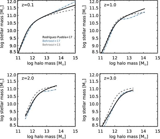
Stellar mass versus halo mass relation derived from abundance matching, shown at several different redshifts as indicated in the panels. The black solid line shows the relation from Rodriguez-Puebla et al. (2017), which is the fiducial relation used in this work. The blue dot–dashed line and grey dashed line show the relations derived by Behroozi et al. (in preparation) and Behroozi et al. (2013b), respectively.

Open in new tab Download slide

The SMHM relation has dispersion both due to intrinsic scatter in the relation, and due to observational stellar mass errors. Following RP17, we adopt an intrinsic scatter of σ_h = 0.15 dex and a scatter due to observational stellar mass measurement errors of σ_* = 0.1 + 0.05z, where z is redshift. These choices are consistent with the constraints summarized by Tinker et al. (2017). Operationally, we assign 〈log m_*(M_h)〉 from equations 25–33 of RP17, then add to this number a Gaussian random deviate with standard deviation |$\sigma _{T} = (\sigma _{h}^2 + \sigma _*^2)^{1/2}$|⁠. For halo mass, we use the maximum mass along the halo's history, as in RP17. For distinct (non-sub) haloes, this is generally equivalent to the standard virial mass, while for sub-haloes, this has been shown to produce better agreement with clustering measurements. We assume that satellite galaxies obey the same SMHM relationship as central galaxies. While this may not be precisely correct (Zheng et al. 2005), the great majority of galaxies in the mass range we study are central galaxies, so our results should not be very sensitive to this assumption.

Consistency with observed clustering measurements is an important check of SHAMs. A similar SHAM has been shown to be consistent with clustering measurements by Rodríguez-Puebla et al. (2015), and the updated RP17 SHAM is also consistent with observed galaxy two-point correlation functions from z ∼ 0.1 to 1 (Rodriguez-Puebla, private communication).

With stellar masses assigned to each of our haloes, we can then use a simple but robust approach to constrain the median relationship between galaxy size and halo size. We bin our SHAM sample in stellar mass and compute the medians of the halo radius 〈R_h(m_*)〉 and spin times halo radius 〈λR_h(m_*)〉. Similarly, we compute the median observed galaxy size in the same stellar mass bins, 〈r_e(m_*)〉. We then obtain SRHR = 〈r_e〉/〈R_h〉 and SRHRλ = 〈r_e〉/〈λR_h〉. We use medians as our default, but also repeat our analysis using means, finding qualitatively similar conclusions.

We note that a distinction is frequently made between spheroid- and disc-dominated galaxies, or star-forming and quiescent galaxies, in discussing their sizes. Some previous studies (e.g. K13, H17) present results for the relationship of galaxy size to halo size for samples of different galaxy types, using a common abundance matching relation. We make a deliberate choice not to divide galaxies by type in our study, as there is strong evidence that star-forming/dis-dominated galaxies and quiescent/red galaxies have significantly different SMHM relations (e.g. Rodríguez-Puebla et al. 2015). Moreover, it is possible that disc- and spheroid-dominated galaxies may arise from haloes with different spin parameter distributions. In order to avoid making assumptions about possible differences in the properties of haloes that host different types of galaxies, we simply compute our results in stellar mass bins.

Another interesting issue is whether the size–mass relation for galaxies depends on the larger scale environment (e.g. on scales larger than the halo virial radius). Similarly, looking into this issue requires knowledge of whether the SMHM relation is universal or depends on environment. We intend to investigate this is future works.

3 OBSERVATIONAL DATA

3.1 GAMA

To characterize nearby galaxies, we make use of the catalogues from Data Release 2 (DR2) of the GAMA survey ( Liske et al. 2015), covering 144 deg². GAMA is an optically selected, multiwavelength survey with high spectroscopic completeness to r < 19.8 mag (two magnitudes deeper than the Sloan Digital Sky Survey; SDSS). We make use of stellar mass estimates from Taylor et al. (2011), and structural properties (semimajor axis half-light radius and Sérsic parameter) from the analysis of Kelvin et al. (2012) using the galfit code (Peng et al. 2002). We restrict our sample to a redshift range 0.01 < z < 0.12 and require r-band galfit quality flag = 0 (good fits only). In addition, we discard galaxies with Sérsic index n_s < 0.3 or n > 10, as these are typically signs of unreliable fits, and we also exclude galaxies with sizes r_e < 0.5 FWHM. The full width at half-maximum (FWHM) is set by the seeing of SDSS, for which we adopt an average value of 1.5 arcsec. We adopt the results of structural fits in the observed r band (due to the relatively small redshift range probed by GAMA, k-corrections should not be needed). After these cuts, we have 13 771 galaxies in our GAMA sample.

3.2 CANDELS

CANDELS is anchored on HST/WFC3 observations of five widely spaced fields with a combined area of about 0.22 deg². An overview of the survey is given in Grogin et al. (2011) and Koekemoer et al. (2011). The data reduction and cataloging for each of the fields is presented in Nayyeri et al. (2017, COSMOS), Stefanon et al. (2017, EGS), Barro et al. (in preparation, GOODS-N), Guo et al. (2013, GOODS-S) and Galametz et al. (2013, UDS). The primary CANDELS catalogues are selected in F160W (H band), and CANDELS has a rich ancillary multiwavelength data set extending from the radio to the X-ray (see Grogin et al. 2011 for a summary). Photometric redshifts have been derived as described in Dahlen et al. (2013). We make use of the z_best redshift from the CANDELS catalogue, which selects the best available redshift estimate from spectroscopic, 3D-HST grism based, and photometric redshifts. Stellar masses are estimated by fitting the spectral energy distributions as described in Mobasher et al. (2015), with further details for each field given in Santini et al. (2015) for GOODS-S and UDS, Stefanon et al. (2017) for EGS, Nayyeri et al. (2017) for COSMOS and Barro et al. (in preparation) for GOODS-N. The stellar masses were derived assuming a Chabrier (2003) stellar initial mass function.

Structural parameters were derived using galfit as described in van der Wel et al. (2012). The fits were done using a single-component Sérsic model. The effective radius that we use is the semimajor axis of the ellipse that contains half of the total flux of the best-fitting Sérsic model. We select CANDELS galaxies with apparent magnitude H₁₆₀ < 24.5, PHOTFLAG=0 (good photometry), 0 < z_best ≤ 3.0, galfit quality flag = 0 (good fits) and stellarity parameter CLASS_STAR <0.8. We discard galaxies with relative size errors greater than a factor 0.3. There are 49 241 galaxies in the catalogue with H₁₆₀ < 24.5 and 0 < z_best ≤ 3.0. Adding the photometry and stellarity criteria brings the number down to 45 015. The galfit quality cut further reduces the number to 38 610, and the error clipping to 28 840. Note that we have repeated our analysis without clipping the size errors, and using a magnitude limit of 25.5. Our results do not change significantly.

In this work, we use the sizes measured from the observed H₁₆₀ image, and apply structural k-corrections to convert to rest-frame 5000 Å sizes. We apply the redshift and stellar mass dependent correction for ‘late-type’ galaxies given by vdW14 (their equation 1) to galaxies with Sérsic index n_s < 2.5, and apply a constant correction Δlog R_eff/Δlog λ_eff = −0.25 to galaxies with n_s > 2.5 (again following vdW14, for ‘early-type’ galaxies). Although vdW14 use a UVJ colour cut, rather than Sérsic index, to divide early- and late-type galaxies, and use sizes derived from the J₁₂₅ image rather than the H₁₆₀ one at z < 1.5, we have confirmed that when we follow exactly the same procedure as vdW14, we get results that are indistinguishable for the purposes of this paper (these alternate choices were adopted simply for convenience). Moreover, as we show later, our results for the size–mass relation of galaxies from 3 ≲ z ≲ 0.2 are in very good agreement with the published size–mass relations from vdW14 and with the independent analysis of H17. Basic estimates of the redshift and colour-dependent stellar mass completeness limits are given in vdW14. It is important to keep in mind that our sample may be somewhat incomplete in the three highest redshift bins. We carry out a more detailed assessment of the magnitude, size, colour, and Sérsic-dependent completeness of the CANDELS sample in Somerville et al. (in preparation).

We convert the GAMA and CANDELS angular half-light radii to physical kpc using the same cosmological parameters quoted above (all sizes in this work are in physical, rather than comoving, coordinates).

3.3 Converting from projected light to 3D stellar mass sizes

The radii that we obtain from the GAMA and CANDELS catalogues described above are projected (2D) half-light radii in the rest-frame r or V band (approximately). We can simply relate this quantity directly to halo properties such as virial mass and virial radius, which is useful empirically. However, in order to gain more insight into the physical meaning of these relationships, it is useful to attempt to convert these sizes into 3D, stellar half-mass radii.

For simplicity, we assume that the projection from 3D to 2D and the correction from rest-frame optical light to stellar mass can be written as two separate terms,

\begin{equation} r_{\rm e, obs} = f_{p} \,\, f_{k}\,\, r_{\rm *, 3D}, \end{equation}

(4)

where r_e,obs is the observed (projected) effective radius of the light in a fixed rest-frame band along the semimajor axis, and r_*,3D is the 3D half-mass radius of the stellar mass distribution. The factor f_p corrects for projection and f_k accomplishes the structural k-correction.³

For a face-on razor thin, transparent disc, f_p = 1. For a spheroid, f_p = 0.68 for a de Vaucouleurs profile (n_s = 4) and f_p = 0.61 for an exponential profile (n_s = 1; Prugniel & Simien 1997). For thick discs or flattened spheroids, f_p would be intermediate between these values. Clearly, the dependence of f_p on galaxy shape could introduce an effective dependence of r_e,obs/r_*,3D on stellar mass and/or redshift, as the mix of galaxy shapes depends on both of these quantities (van der Wel et al. 2009, 2014b). van der Wel et al. (2014b) showed that the fraction of elongated (prolate) galaxies increases towards higher redshifts (up to z ∼ 2) and lower masses, such that at z ∼ 1, at least half of all galaxies with stellar mass |$10^9\,\,{\,\,{\rm M}_{{\odot}}}$| are elongated. This is also seen in numerical hydrodynamic simulations (Ceverino, Primack & Dekel 2015). Dust could also affect the relationship between 3D and projected radius.

Regarding the structural k-corrections, Dutton et al. (2011b) quote f_k ∼ 1.3 for low-redshift discs in the V band. Szomoru et al. (2013) compute stellar mass distributions using a single colour, for a sample of a couple hundred galaxies with HST observations as well as some nearby galaxies from SDSS, covering a redshift range 0 < z < 2.5. They find average corrections in the rest g-band log (r_*/r_g) ∼ −0.12 at z = 0, −0.14 at 0.5 < z < 1.5 and −0.10 at 1.5 < z < 2.5. They did not find any strong trends with redshift, galaxy morphology or specific star formation rate (sSFR) although again their sample was small. They saw hints of smaller values of log (r_*/r_g) for high Sérsic, quiescent galaxies.

Wuyts et al. (2012) computed stellar mass distributions using pixel-by-pixel SED fitting with an earlier release of CANDELS/3D-HST. They show distributions of r_e for rest V-band light and for stellar mass in two redshift bins: 0.5 < z < 1.5 and 1.5 < z < 2.5. They find that the distribution of half-mass radii is shifted by 0.1–0.2 dex with respect to that of the half-light radii. There does not seem to be evidence for strong redshift evolution, and they do not discuss any dependence on galaxy mass or type.

Lange et al. (2015) discuss the change in size from u through K band for the GAMA sample. To first order one can assume that the stellar mass effective radius is the same as the K-band light effective radius. From g to K band, Lange et al. (2015) find a decrease in radius of 16 per cent at |$m_* \sim 10^{9}{\,\,{\rm M}_{{\odot}}}$| and 13 per cent at |$m_* \sim 10^{10}{\,\,{\rm M}_{{\odot}}}$| for ‘late-type’ galaxies. For ‘early-types’, they again find 13 per cent at |$m_* \sim 10^{10}{\,\,{\rm M}_{{\odot}}}$| and 11 per cent at |$m_* \sim 10^{11}{\,\,{\rm M}_{{\odot}}}$|⁠. So again, they find weak dependence of f_k on type and stellar mass. In summary, values of f_k in the literature range from ∼1.12 to 1.5. Values are perhaps slightly smaller for quiescent/early-type galaxies, but there does not seem to be evidence for a strong trend with mass or redshift.

For purposes of this work, we adopt a rough best guess value of (f_pf_k)_disc = (1*1.2) = 1.2 for discs, and (f_pf_k)_spheroid = (0.68 * 1.15) = 0.78 for spheroids. To get a rough idea for how these corrections might affect our results, we apply (f_pf_k)_disc to estimate r_3D,* for galaxies with Sérsic index n_s < 2.5, and use (f_pf_k)_spheroid for galaxies with n_s > 2.5. Although it is known that there is not a perfect correspondence between galaxy shape and Sérsic index, this at least gives us a first approximation for how the dependence of galaxy type on stellar mass and redshift might affect the trends we wish to study.

For reference, we show the observed (projected light) size–mass relations and our derived 3D stellar half-mass radius relations for both the GAMA and CANDELS samples in Figs A1 and A2. A comparison between the observational size–mass relations used in this work and the literature is discussed in Appendix A.

Lastly, we note that for a thin exponential disc, the scale radius r_d given in equation (2) is related to the half-mass radius via r_1/2 = 1.68r_d.

4 RESULTS

4.1 Results from the GAMA survey at z = 0.1

Fig. 2 shows the size–mass relation at z = 0.1 from the GAMA survey, compared with the SHAM assuming r_e = 0.5λR_h. Note that Lange et al. (2015) show that a stellar mass limit of |$2.5 \times 10^9{\,\,{\rm M}_{{\odot}}}$| yields a colour-unbiased, 97.7 per cent complete sample out to the adopted redshift limit. This limit is indicated in Fig. 2 by the vertical line. It is somewhat remarkable how well a mass-independent value of SRHRλ reproduces the average size–mass relation over many orders of magnitude in stellar mass. This result reproduces and confirms the results already presented by K13. The median value of the spin parameter in Bolshoi–Planck is 〈λ〉 = 0.036, so SRHRλ = 0.5 corresponds to r_e/R_h = 0.018 which is fairly close to the value found by K13 (r_e/R_h = 0.015). Also note the steeper slope of the scaling relation between halo virial mass and halo virial radius, compared to the observed size–mass relation for galaxies. In this simple model, the change in slope is entirely due to the slope of the SMHM relation.

Figure 2.

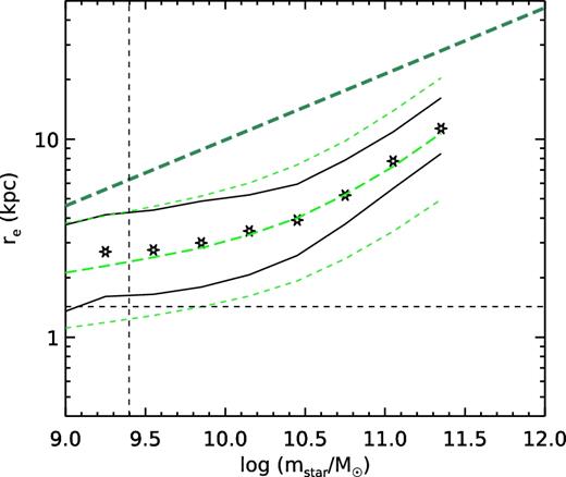
The relationship between stellar mass and effective radius at z ∼ 0.1. The green dashed lines show the median and 16 and 84th percentiles in bins of stellar mass for the SHAM model, assuming r_e = 0.5λR_h. The black stars and lines show the median and 16 and 84th percentiles of the 3D half stellar mass radius for the GAMA z = 0.1 sample. The horizontal dashed line shows the minimum size of galaxies that can be resolved at the upper redshift limit of the GAMA sample used here. The dashed vertical line shows the 97.7 per cent stellar mass completeness limit for the GAMA sample. The dark green dashed line shows the scaling relation for halo virial mass and halo virial radius (both scaled down by a factor of 10), illustrating that the size–mass relation for haloes has a much steeper slope than that for galaxies.

Open in new tab Download slide

In Fig. 3, we show the ratio of the median observed size in a stellar mass bin to the median value of R_h or λR_h in that same bin, again using the SHAM to link halo mass to stellar mass. We also show the same quantity for the estimated de-projected stellar half-mass radii. This is simply another way of showing the results already seen above: SRHR and SRHRλ are nearly independent of stellar mass and have values of approximately SRHR = 0.018 and SRHRλ = 0.5. The apparent decrease in the value of SRHR or SRHRλ towards larger stellar masses appears to be mitigated by the correction from projected to 3D size. We note that, as found in many previous studies, we do not see any significant dependence of the spin parameter λ on halo mass in the Bolshoi–Planck simulations.

Figure 3.

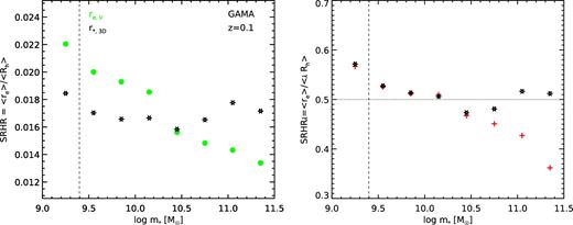
Results from the GAMA survey at z = 0.1. Left-hand panel: Median galaxy radius divided by the median value of the halo virial radius (SRHR). Filled green circles show SRHR for the observed (projected) r-band half-light radius r_e. The dashed vertical line shows the 97.7 per cent stellar mass completeness limit for the GAMA sample. Black star symbols show the SRHR for the estimated 3D stellar half-mass radius (r_*,3D). Right-hand panel: Median galaxy radius divided by the median value of the spin parameter times the halo virial radius (SRHRλ). Black stars show the fiducial results, while red crosses show the results we would obtain if we did not include scatter in the SMHM relation. It is striking that the ratio between galaxy size and halo size remains so nearly constant over a wide range in stellar mass.

Open in new tab Download slide

Fig. 4 shows the conditional size distributions (for observed half-light radii) in stellar mass bins for the GAMA sample. We have applied a standard V_max completeness correction, as GAMA starts to become incomplete below stellar masses of about |$10^{10}{\,\,{\rm M}_{{\odot}}}$|⁠. We show the size distributions separately for galaxies with Sérsic n_s < 2.5, which should correspond approximately to disc-dominated galaxies, and with Sérsic n_s > 2.5, which should be spheroid dominated. We show this to emphasize that in the lowest stellar mass bins we consider, the distribution is dominated by n_s < 2.5, presumably disc-dominated galaxies, while in the highest stellar mass bins shown, the distribution is dominated by n_s > 2.5 spheroid-dominated galaxies. The fraction of galaxies in the bin with n_s < 2.5 is shown in each panel.

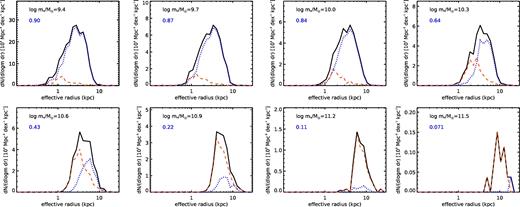
$Distribution functions in bins of stellar mass for the (2D) effective radius in the GAMA survey. The black solid lines show the distribution for all galaxies, the blue dotted lines show disc-dominated (ns < 2.5) galaxies, and the red dashed lines show spheroid-dominated (ns > 2.5) galaxies. The blue number in the upper left corner of each panel indicates the fraction of galaxies in that mass bin that are disc dominated (ns < 2.5).$

Figure 4.

Distribution functions in bins of stellar mass for the (2D) effective radius in the GAMA survey. The black solid lines show the distribution for all galaxies, the blue dotted lines show disc-dominated (n_s < 2.5) galaxies, and the red dashed lines show spheroid-dominated (n_s > 2.5) galaxies. The blue number in the upper left corner of each panel indicates the fraction of galaxies in that mass bin that are disc dominated (n_s < 2.5).

Open in new tab Download slide

Fig. 5 shows the conditional size distributions P(r_e|m_*) in stellar mass bins from GAMA (using the corrected 3D stellar half-mass radii), compared with the corresponding distributions of P(R_h|m_*) and P(λR_h|m_*) in stellar mass bins from the SHAM. The distribution P(λR_h|m_*) in the SHAM is very close to lognormal, as is well known to be the case for the spin parameter in cosmological simulations (e.g. Bullock et al. 2001). In the lower stellar mass bins (log (m_*/M_⊙) ≲ 10.8, the distribution of P(R_h|m_*) is narrower than the observed distribution P(r_e|m_*), while the dispersion in the distribution P(λR_h|m_*) matches the observed dispersion in P(r_e|m_*) quite well. In the higher stellar mass bins, the dispersion in P(R_h|m_*) is already as large as the dispersion in P(r_e|m_*), while the dispersion in P(λR_h|m_*) is larger than the observed dispersion. We discuss the interpretation of this result further in Section 5.4.3.

Figure 5.

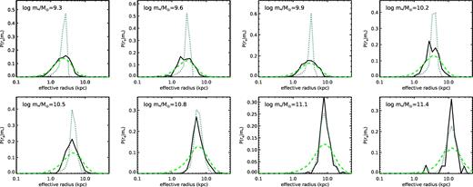
Conditional probability distributions for effective radius in bins of stellar mass, at z ∼ 0.1. Stellar mass bins increase from left to right and top to bottom, as indicated in the panel labels. Black solid lines show the distribution of estimated 3D half stellar mass radius (r_3D,*) from the GAMA observations. Green dashed lines show distributions of SRHRλ(λR_h) from the SHAMs using a constant value of SRHRλ = 0.5. Dark green dotted lines show distributions of SRHR R_h. This result places limits on the galaxy to galaxy dispersion in SRHR and SRHRλ.

Open in new tab Download slide

4.2 Results from the CANDELS survey at 0.1 < z < 3.0

We now investigate constraints on the dependence of SRHR and SRHRλ on stellar mass at different cosmic epochs. To do this, we use the same SHAM approach, applied to mock CANDELS light-cones extracted from the Bolshoi–Planck simulation. We consider redshift bins 0.1–0.5, 0.5–1.0, 1.0–1.5, 1.5–2.0, 2.0–2.5 and 2.5–3.0. Fig. 6 shows SRHR, the ratio of median observed effective radius r_e or de-projected half stellar mass radius r_*,3D to the median value of R_h in stellar mass bins, for these six redshift bins. At z = 0.1, we found that SRHR is nearly constant across the full range of stellar masses considered in our analysis. However, SRHR seems to gain a stronger dependence on stellar mass as we move towards z ∼ 3, with more massive galaxies having lower values.

Figure 6.

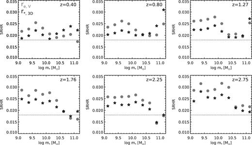
The median observed radius in a stellar mass bin divided by the median value of halo radius R_h, from z ∼ 0.1 to 3 (the values indicated in each panel are the volume mid-points of each bin). Filled circles (grey) and stars (black) show results for the observed (projected) half-light radius r_e and the 3D half stellar mass radius (r_3D,*). The dotted horizontal grey line shows the average z = 0.1 value of SRHR from our analysis of the GAMA survey. SRHR has a stronger dependence on stellar mass in the higher redshift bins, and we see hints of a mild decrease of SRHR with cosmic time.

Open in new tab Download slide

Fig. 7 shows SRHRλ, the ratio of median de-projected stellar mass weighted radius r_*,3D to the median value of λR_h in stellar mass bins, for six redshift bins as before. We show results for both definitions of spin parameter (Peebles and Bullock). We can see that any conclusions about the evolution of SRHRλ depend to a significant degree on which spin definition is adopted, although trends with stellar mass are not affected. This is because in the Bolshoi–Planck simulations, the Peebles and Bullock spin parameters evolve differently with cosmic time (as shown by Rodríguez-Puebla et al. (2016b) and in Appendix B of this paper). We discuss the possible reasons for the different evolution of the two definitions of spin parameter in Section 5.1.2 and in the appendix.

Figure 7.

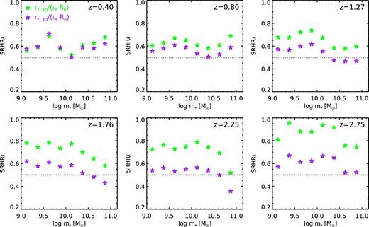
The median observed radius in a stellar mass bin divided by the median value of halo radius R_h times halo spin (SRHRλ), from z ∼ 0.1 to 3 (the values indicated in each panel are the volume mid-points of each bin). Here, we use the 3D half stellar mass radius (r_3D,*). Green symbols show the results using the Peebles spin definition, and purple show the results using the Bullock spin. The dotted horizontal grey line shows the average z = 0.1 value of SRHRλ from our analysis of the GAMA survey.

Open in new tab Download slide

In Fig. 8, we plot our results for SRHR and SRHRλ for two bins in stellar mass |${\sim } 10^{10}{\,\,{\rm M}_{{\odot}}}$| and |${\sim } 10^{11}{\,\,{\rm M}_{{\odot}}}$| as a function of cosmic time since the big bang. We again show our results for SRHRλ for both definitions of the spin parameter (Peebles and Bullock). For galaxies with |$m_* \lesssim 10^{10.5}{\,\,{\rm M}_{{\odot}}}$|⁠, when using the Peebles spin, SRHRλ declines by about a factor of 1.8 over the redshift range of our study. Using the Bullock definition of spin, SRHRλ in this mass range is consistent with being constant in time. For more massive galaxies, SRHRλ is nearly constant, or increases slightly, over cosmic time within the CANDELS sample. The value of SRHR and SRHRλ derived from GAMA at z ∼ 0.1 is about a factor of 1.4 lower than the CANDELS results from the lowest redshift bin. This suggests that there may be a systematic offset between the size or stellar mass estimates in GAMA and CANDELS for massive galaxies.

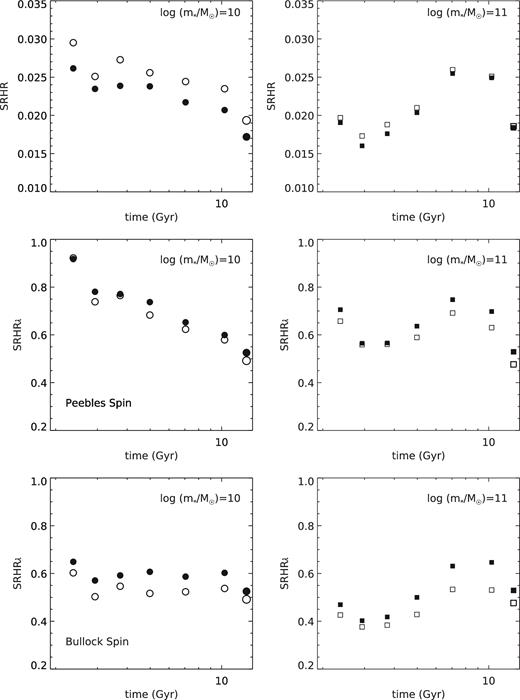
$Time evolution of SRHR and SRHRλ, the ratio between median r*,3D and Rh or λRh, for two different stellar mass bins: $10^{9.75}\,\,{\,\,{\rm M}_{{\odot}}}< m_* < 10^{10.25}\,\,{\,\,{\rm M}_{{\odot}}}$ (left; filled) and $10^{10.75}\,\,{\,\,{\rm M}_{{\odot}}}< m_* < 10^{11.25}\,\,{\,\,{\rm M}_{{\odot}}}$ (right; filled). Top row: SRHR. Middle row: SRHRλ using the Peebles spin definition; bottom row: SRHRλ using Bullock spin. The ratio of the mean quantities is shown by the open symbols – using means instead of medians results in slightly different numerical values, but does not change any of the trends.$

Figure 8.

Time evolution of SRHR and SRHRλ, the ratio between median r_*,3D and R_h or λR_h, for two different stellar mass bins: |$10^{9.75}\,\,{\,\,{\rm M}_{{\odot}}}< m_* < 10^{10.25}\,\,{\,\,{\rm M}_{{\odot}}}$| (left; filled) and |$10^{10.75}\,\,{\,\,{\rm M}_{{\odot}}}< m_* < 10^{11.25}\,\,{\,\,{\rm M}_{{\odot}}}$| (right; filled). Top row: SRHR. Middle row: SRHRλ using the Peebles spin definition; bottom row: SRHRλ using Bullock spin. The ratio of the mean quantities is shown by the open symbols – using means instead of medians results in slightly different numerical values, but does not change any of the trends.

Open in new tab Download slide

We now investigate the conditional distributions of galaxy radius in stellar mass bins out to z ∼ 3. Fig. 9 shows the conditional size distributions in bins of stellar mass and redshift from CANDELS. Note that this diagram is similar to Fig. 10 of vdW14, and the results appear similar, although here we show the estimated deprojected stellar half-mass radii rather than the projected half-light radii. We also show conditional distributions of the quantity SRHRλ × (λR_h) from the SHAM, where we have used the redshift and stellar mass dependent values of SRHRλ derived above, and shown in Fig. 7, to shift the median of the SHAM distribution to match that of the observed distributions. In this way, we can compare the shape and width of the distributions in detail. As before, the SHAM distributions and their dispersions match the observed conditional size distributions remarkably well. We show here the results for the Peebles definition of the spin parameter, but the distribution shapes are very similar for the Bullock definition. We discuss the significance of these results in Section 5.4.3.

Figure 9.

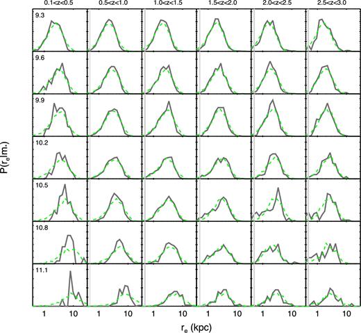
The conditional probability distribution for effective radius r_e in bins of stellar mass and redshift. Grey solid lines show the distributions of the estimated 3D half stellar mass radii (r_*,3D) from CANDELS. Vertical grey lines show the physical size corresponding to one F160W pixel in the drizzled image (0.06 arcsec), at the lower and upper limit of the redshift bin. Green dashed lines show distributions P(λR_h|m_*) from the SHAM (using the Peebles spin definition). The SHAM distributions have been shifted horizontally to match the medians of the observed distributions, to emphasize the comparison of the shapes of the distribution functions.

Open in new tab Download slide

Figure 10.

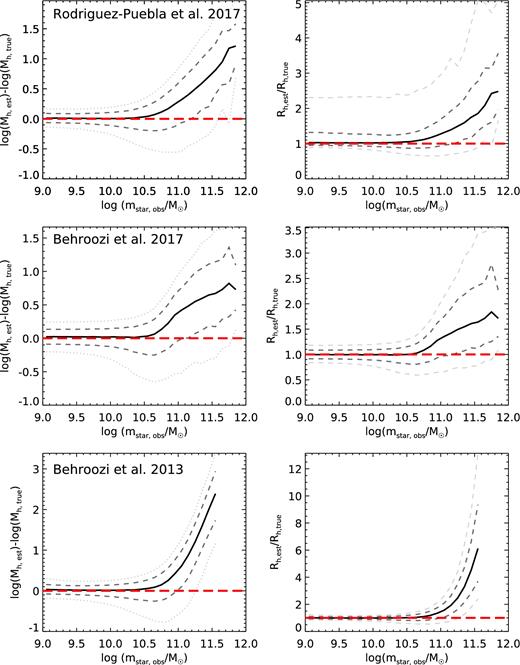
A test of the accuracy of recovering halo mass and radius estimates from backwards modelling, based on applying this method to a mock catalogue in which the true halo masses and radii are known. Different panels show the results from mock catalogues created with different SHAM models, as indicated on the panels. The left column shows the difference between the log of the halo mass estimated by backwards modelling and the log of the true halo mass, and the right-hand panels show the ratio of estimated to true halo virial radius. Red lines indicate equality, solid black lines show the medians, medium grey dashed lines show the 16th and 84th percentiles and light grey dashed lines show the 2nd and 98th percentiles. The median recovered halo mass and radius is fairly accurate below the ‘turnover’ in the SMHM relation slope, but above this critical mass, the errors can become very large. The error in recovering the halo mass depends on the slope of the SMHM relation and the scatter in the SMHM relations due to intrinsic dispersion and stellar mass errors.

Open in new tab Download slide

5 DISCUSSION

In this section, we discuss the main caveats and uncertainties in our analysis, compare the ‘forward’ and ‘backwards’ modelling approaches, compare our results and conclusions with those of previous studies, and discuss possible physical interpretations of our results. Some readers may wish to skip directly to Section 5.4 for the discussion of the physical interpretation of our results.

5.1 Main caveats and uncertainties

Our analysis makes use of, on the one hand, observational estimates of galaxy stellar mass, redshift and radial size (and, secondarily, morphological type), and on the other, predictions of the mass, radius and spin parameters of dark matter haloes from a cosmological simulation.

5.1.1 Halo properties and SMHM relation

There are several important caveats to note regarding the halo properties and SMHM relation. First, the halo masses, virial radii and spin parameters are taken from dissipationless N-body simulations, which do not include the effect of baryons on halo properties. Studies that do include baryons and the associated feedback effects have shown that baryonic processes can modify the virial mass and spin parameter of dark matter haloes by up to 30 per cent (Munshi et al. 2013; Teklu et al. 2015) and the magnitude of these effects may depend on halo mass. Therefore, the actual ratio of galaxy size to halo size and spin parameter may differ from the values quoted here.

Second, specific properties of dark matter haloes such as mass, radius and spin parameter depend on the definition used. See Appendix B for a detailed description and illustration of different halo mass, radius and spin definitions.

How would our results change had we adopted a different halo definition? The halo definition impacts several aspects of our calculation. Recall that we have used the definition M_vir,crit as given in Section 2. Haloes with a fixed value of M_200,crit are less abundant (have a lower volume density) than haloes with the same numerical value of M_vir,crit. Similarly, haloes with a fixed value of M_vir,crit are less abundant than haloes with the same numerical value of M_200,b. This means that galaxies with a given stellar mass (and observed number density) will be assigned larger and larger halo masses depending on the halo definition used, from M_200,crit → M_vir,crit → M_200,b → M_vir,b. Moreover, the virial radius for a given halo mass increases as we go from M_200,crit → M_vir,crit → M_200,b → M_vir,b. Since r_e for a given m_* is fixed by the observed relation, all of this implies that r_e/R_h would be largest for the M_200,crit definition and smallest for the M_vir,b definition. Our favoured definition is in the middle. Furthermore, we expect λ to increase slightly as we go from M_200,crit → M_vir,crit → M_200,b → M_vir,b. This means the difference in r_e/(λR_h) will be even a bit larger from one halo definition to another. To accurately fully estimate the effects of changing the halo definition, we would need to redo the abundance matching and remeasure λ consistently for each definition, which is beyond the scope of this paper. However, a crucial point is that we have been very careful to use a consistent halo mass definition in all aspects of our study.

The choice of halo definition is in some sense arbitrary. Yet, one can ask which definition is the most physically relevant for tracking quantities that are relevant to galaxy formation, such as the accretion rate of gas into the halo. Some recent works that examined structure formation in dark matter only simulations have pointed out that defining the halo relative to an evolving background density leads to apparent growth of the halo mass even as the physical density profile of the interior of the halo remains unchanged, an effect that has been termed ‘pseudo-evolution’ (Busha et al. 2005; Diemer, More & Kravtsov 2013). This suggests that this mass growth should not be associated with physical accretion of matter into the halo. However, some more recent studies that have examined simulations including baryonic physics find that the accretion rate of gas into the central part of haloes (on to forming galaxies) tracks the growth of the virial radius quite well (Dekel et al. 2013; Wetzel & Nagai 2015). This implies that while pseudo-evolution is a relevant concept for dark matter, not so for baryons, which can shock and cool. The work of both Dekel et al. (2013) and Rodríguez-Puebla et al. (2016a) support the physical relevance of the halo mass definition adopted here, and it is quite similar to the 200 times background definition that was found to trace gas accretion by Wetzel & Nagai (2015).

Another important caveat is the adopted SMHM relation, which plays a critical role in our analysis. As already noted, the abundance of dark matter haloes as a function of their mass depends on the halo mass definition, but it also depends on the method used to identify haloes and sub-haloes in the N-body simulation. The cumulative halo mass function at z = 0 differed by ±10 per cent across the 16 halo finders tested in Knebe et al. (2011). However, much larger differences between different halo finders can arise at high redshift (Klypin, Trujillo-Gomez & Primack 2011). Phase-space-based methods such as the ROCKSTAR halo finder used here tend to be the most robust (Knebe et al. 2011). In deriving the SMHM relation, there are also subtleties regarding how sub-haloes are treated: whether to use their properties at infall or at the time they are identified (these can differ substantially due to tidal stripping), and whether sub-haloes/satellites obey the same SMHM relation as central galaxies. As noted above, sub-haloes/satellites should be sufficiently sub-dominant in our sample that these details will not have a large impact on our results.

The main reason for systematic differences between SMHM relations quoted in the literature is in fact the lack of convergence between different observational determinations of the stellar mass function. This is most acute for very massive nearby galaxies (Bernardi et al. 2013; Kravtsov, Vikhlinin & Meshscheryakov 2014) and also at high redshift – even at z ∼ 1 there is a lack of convergence regarding the low-mass slope of the stellar mass function (see e.g. Moster et al. 2010). The SMHM relation used in this work is based on a very recent and complete compilation of stellar mass functions, and adopts the same cosmological parameters as in our work. We have confirmed that when we apply the RP17 SMHM relation with our adopted scatter to our halo catalogues, we reproduce the GAMA stellar mass function at z = 0.1 and the CANDELS stellar mass functions at z ∼ 0.1–3. As we showed in Fig. 1, several recent determinations of the SMHM relation are in good agreement over the mass range relevant to our study (⁠|$10^{9} \lesssim m_* \lesssim 10^{11}{\,\,{\rm M}_{{\odot}}}$|⁠). We further note that the differences between the RP17 and B17 z = 0.1 SMHM relation seen in Fig. 1 do not significantly affect our results, because we focus on galaxies less massive than a few |$10^{11}{\,\,{\rm M}_{{\odot}}}$|⁠, where the differences are small. However, adopting a larger scatter in the SMHM relation leads to larger values of SRHR at high stellar masses (m_* ≳ 10^10.5), as more galaxies hosted by lower mass haloes are scattered into these bins.

5.1.2 Definition of halo spin parameter

We have seen that our results for the evolution of SRHRλ are quite different for two commonly used definitions of the spin parameter λ. As shown by Rodríguez-Puebla et al. (2016b), at z = 0 the distributions of λ_B and λ_P peak at nearly the same value, but λ_B has a more pronounced tail to larger values (see fig. 21 of Rodríguez-Puebla et al. 2016b). However, λ_P increases from z ∼ 3 to 0, while λ_B decreases slightly over this interval. Very similar results are shown in a recent analysis of the Illustris simulations by Zjupa & Springel (2017). This explains why we found milder evolution in SRHRλ when using the Bullock definition λ_B.

We discuss possible reasons for the different behaviour of λ_P and λ_B in Appendix B. We conclude that this is likely due to a combination of changing halo density profiles (concentration), deviation of haloes from perfect spheres, and/or changes in halo kinematics (deviation from circular orbits). This brings up further concerns regarding the basis of simple analytic models of disc formation, which assume that all halo particles are on circular orbits.

Which definition of halo spin is more physically relevant to the question at hand, namely galaxy sizes? We feel that this is not currently clear. In some sense, the Peebles definition appears to capture some real and potentially relevant evolution in halo structure and kinematics. Moreover, it is the Peebles definition of λ that properly comes in to somewhat more sophisticated analytic models of disc formation (e.g. Mo et al. 1998; Somerville et al. 2008b), i.e. equation (6) below. Zjupa & Springel (2017) find that the Peebles definition is more robust than the Bullock definition for haloes defined by the friends-of-friends method. The relevance of either quantity to observed galaxy sizes should be explored further using detailed numerical simulations of galaxy formation, but the potentially significant differences between these two definitions should be kept in mind.

5.1.3 Observational measurements

Analogous to the problem of defining a halo, there is no unique way to define the total amount of light within a galaxy, as galaxies do not have sharp edges. This necessarily leads to an ambiguity in how the half-light radius is defined, as it is defined relative to the total amount of light. Commonly used metrics include isophotal magnitudes (and sizes), Petrosian or Kron magnitudes and sizes, model magnitudes and sizes, and the curve-of-growth method (Bernardi et al. 2014; Curtis-Lake et al. 2016). Here, we have used model sizes, where the model is a single component Sérsic profile. Some galaxies are not well fitted by a single component Sérsic profile, and one might expect our method to do poorly in these cases. In the local Universe, the largest discrepancy in total luminosity, stellar mass and size is for very massive giant elliptical galaxies (Bernardi et al. 2013, 2014). Our CANDELS sample is dominated by lower mass galaxies, so that part of our analysis should not be greatly affected by these objects. Model fitting based sizes can also be sensitive to the local background used in the fitting, and to the seeing or point spread function of the image. We adopted the GAMA sample for our study because the methods used to estimate stellar masses and sizes were as similar to those used for CANDELS as any low-redshift sample of which we are aware. In both GAMA and CANDELS, sizes are estimated using the same code (galfit) and single component Sérsic fitting.

Another important note is that some studies (e.g. Shen et al. 2003; Shibuya et al. 2015) have used circularized radii (r_e,circ ≡ q^1/2 r_e,major where q is the projected axial ratio), rather than semimajor axis radii. Because galaxy axial ratios can depend on stellar mass and redshift, this could lead to different conclusions.

Further uncertainties come from the conversion from observed, projected (2D) radii to physical 3D radii, which depends on the shape of the galaxy (flat versus spheroidal). Again, this is probably correlated with stellar mass and may vary with cosmic time. We have attempted to make a crude correction for these dependencies but this should be improved. In a similar vein, we used the empirical corrections of vdW14 to correct from observed-frame H₁₆₀ size to rest-frame 5000 Å size, and then further attempted to convert from observed rest-frame 5000 Å half-light radius to stellar half-mass radius. The mass, redshift, and type dependences of these corrections also remain uncertain and poorly constrained. It should be possible to better account for this in the future by doing pixel-by-pixel SED fitting to measure stellar mass profiles (Wuyts et al. 2012).

5.2 Beware backwards modelling

In the approach used here, we start from an ensemble of dark matter haloes and sub-haloes from theoretical cosmological simulations, and apply empirical relations to map halo mass to stellar mass. We refer to this approach as ‘forward modelling’. An alternative approach, sometimes used in the literature, is what we refer to as ‘backwards modelling’. In backwards modelling, halo masses and radii are derived for an observational sample based on a stellar mass estimate. This is often done by inverting a SMHM relation 〈m_*(M_h)〉 derived from abundance matching. However, this practice can be quite dangerous in the presence of scatter in the underlying SMHM relation, as we now show. From Fig. 1, we can see that above a characteristic value of M_h, the slope of the SMHM relation becomes quite shallow. As a result, a positive deviation in stellar mass Δm_* leads to a larger deviation in the derived halo mass than a corresponding negative Δm_*, leading to a systematic overestimate in halo mass and radius. Moreover, due to Eddington bias, as stellar mass increases above the ‘knee’ in the stellar mass function, an increasing fraction of galaxies with estimated stellar masses in a given stellar mass bin are likely to have been scattered there due to stellar mass errors.

Fig. 10 shows a test based on applying backwards modelling (inversion of a SMHM relation) to a mock catalogue in which the true halo properties are known. We create a mock catalogue of stellar masses based on the Bolshoi–Planck simulation, by applying an assumed SMHM relation with a lognormal scatter in stellar mass at fixed halo mass, as described in Section 2. Our mock catalogue reproduces the observed stellar mass function at z = 0.1. Below the mass scale where the SMHM becomes shallower, the median recovered halo properties are nearly unbiased. However, above this mass scale (⁠|$m_* \simeq 10^{10.5}{\,\,{\rm M}_{{\odot}}}$|⁠), the median recovered halo mass can be overestimated by as much as two orders of magnitude, and the estimated median halo radius can be overestimated by up to a factor of 6. We show this test at z ∼ 0.1 as an illustration, but in detail the errors in recovered parameters will depend on the stellar mass errors and the slope of the SMHM relation.

5.3 Comparison with previous work

Our z ∼ 0.1 analysis of GAMA yields results that are very similar to those of the analysis of K13, which was based on a more heterogeneous low redshift sample that spanned a larger range in stellar mass. Interestingly, in spite of the fact that we used different observational samples and different halo mass definitions, our quantitative conclusions for the low-redshift part of the analysis are very consistent with those of K13: galaxy effective radius is linearly proportional to halo radius with a proportionality factor of ∼0.018 (K13 finds 0.015). However, our physical interpretation of the results is quite different from that of K13, as we discuss further below.

Another recent study that has examined the relationship between galaxy size and halo size using abundance matching is that presented in two papers, Shibuya et al. (2015) and Kawamata et al. (2015). They also analyse the CANDELS+3D-HST sample as well as an additional sample of Lyman-break galaxies. They perform their own galfit fitting procedure to measure the sizes of the CANDELS+3D-HST sample as well as the LBG sample. They find good statistical agreement between their measured sizes and those of vdW14 for the CANDELS+3D-HST sample. They then estimate the dark matter halo radius for each galaxy based on its stellar mass, using the abundance matching relation of Behroozi et al. (2013b), and use this to estimate r_e/R_h. They find values of r_e/R_h = 0.01–0.035, with ‘no strong evolution’ in r_e/R_h from z ∼ 0 to 8. This is broadly consistent with our results. However, there are several differences between their analysis and ours, which make our results difficult to compare in detail. For their main analysis (for which they compute r_e/R_h), galaxies are selected in bins of observed UV luminosity, rather than stellar mass, and sizes are k-corrected to the UV rather than the rest-frame optical. They use a different halo mass definition than we do, and indeed than Behroozi et al. (2013b). They use circularized radii, which as we have noted may have a redshift-dependent relationship with semimajor axis radii. If one looks closely at their fig. 16, focusing on the z ≲ 3 redshift range of our study, there is a difference of almost a factor of 2 between different bins in UV luminosity at fixed redshift. Assuming that UV luminosity roughly traces SFR, it is well known that there is a declining relation between stellar mass and SFR with decreasing redshift (e.g. Speagle et al. 2014, and references therein). One might expect, then, that selecting galaxies at a fixed SFR would select lower mass galaxies at high redshift. Furthermore, even at fixed stellar mass there is a correlation between size and SFR, such that galaxies with below-average SFR for their epoch have smaller sizes (Wuyts et al. 2011; Brennan et al. 2017). Finally, as noted by Behroozi et al. (2013b), the inverse of the fitting formula for the average stellar mass at a given halo mass is not equivalent to the average halo mass at a given stellar mass, because of scatter in the stellar mass–halo mass relation. Shibuya et al. (2015) ‘backward’ model (go from stellar mass to halo mass) while we ‘forward’ model (go from halo mass to stellar mass).

The recent study of H17 is easier to compare with our results, as they use the same CANDELS catalogues and size measurements used in our study. H17 perform a slightly different sample selection from the parent CANDELS catalogues than we do. While we apply a uniform magnitude limit that is appropriate for the CANDELS wide depth (H₁₆₀ < 24.5), H17 apply a fainter magnitude cut in the CANDELS deep and Hubble Ultra-deep field (HUDF) regions. H17 demonstrate the important result that the size distributions for objects in the magnitude range 23.5 < H₁₆₀ < 24.5 in the wide region and HUDF are consistent, confirming that low surface brightness objects or wings are not biasing the size distributions significantly at these magnitudes. As we show in Fig. A2, the size–mass relations that we derive are nearly identical to those obtained from the sample of H17.

In Fig. 11, we show a comparison between our derived values of r_e/R_h, where r_e is the observed (projected) rest-frame 5000 Å half-light radius and R_h is the halo radius, and the median values of r_e/R_h from the analysis of H17. Overall, the results are in excellent agreement, particularly when they repeat their analysis using the same halo mass definition, and a similar SMHM relation, as those adopted in our study. We see hints of a larger drop in r_e/R_h at the highest stellar masses, which may be because the ‘backward modelling’ approach adopted by H17 can tend to overestimate halo mass and radius in the presence of scatter in the SMHM relation (see Section 5.2).

Figure 11.

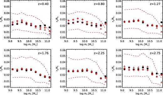
Ratio of (observed, projected) galaxy effective (half-light) radius to halo radius as a function of stellar mass and redshift. Filled circles show the analysis presented in this work. Red crosses show the median values of r_e/R_h from the analysis of H17, using their fiducial halo mass definition and SMHM relation (which are different from ours). Dark red triangles show results from the approach of H17 using our halo definition and the Behroozi et al. (2013b) SMHM relation. The dashed lines show the 16th and 84th percentiles from H17, which estimates R_h for individual galaxies using the ‘backwards modelling’ approach. Our results are in excellent agreement, except at the highest stellar masses, where the differences are likely due to the forward versus backwards modelling approach (see text).

Open in new tab Download slide

H17 show the R_h–r_e relation separately for galaxies with the lowest and highest values of Sérsic index and of sSFR. We are unable to do this in our forward modelling approach. H17 find that the lowest Sérsic (disky) galaxies have larger values of r_e/R_h than the highest Sérsic galaxies. A similar result holds for the highest and lowest sSFR galaxies (the highest sSFR galaxies have larger r_e/R_h). This is consistent with our finding that SRHR is smaller for higher stellar mass bins, which also tend to have larger fractions of high-Sérsic, low-sSFR galaxies. However, we note that H17 have not attempted to perform any correction for the different conversion between projected and 3D radius for flat and round galaxies.

5.4 Physical interpretation

5.4.1 Theoretical expectations for disc sizes

What do our results tell us about the physics that shapes galaxy sizes? We first compare our results with the predictions of the simplest model for disc formation, equation (2). We can re-write this as

\begin{equation} \frac{r_{e}}{\lambda R_{h}} = \frac{1.678}{\sqrt{2}}\,\, f_j, \end{equation}

(5)

where f_j is the ratio of the specific angular momentum of the disc to that of the halo. If this naïve model were correct, then if the specific angular momentum of the stellar disc is the same as that of the halo (f_j = 1), we would have r_e/(λR_h) = 1.18.

Several refinements to this simplest model have been presented in the literature. First, dark matter haloes that form in dissipationless N-body simulations in the ΛCDM paradigm do not have singular isothermal density profiles, but are better characterized by the Navarro–Frenk–White (NFW; Navarro, Frenk & White 1997) functional form. Secondly, in the absence of non-gravitational energy injection, self-gravity from the baryons that collect in the centre of the dark matter halo following cooling and dissipation should lead to contraction, leading to discs that are smaller than the naïve model would predict. The degree of contraction can be estimated using the ‘adiabatic invariant’ approximation (e.g. Blumenthal et al. 1986; Flores et al. 1993; Mo et al. 1998). In this formalism, the contraction factor depends on the halo concentration, the disc mass fraction and the halo spin parameter, where more concentrated haloes, heavier discs, and lower spin parameters lead to more contraction (see Dutton et al. 2007; Somerville et al. 2008b).

In these slightly more sophisticated models, we now obtain (Mo et al. 1998; Somerville et al. 2008b):

\begin{equation} \frac{r_{e}}{\lambda R_{h}} = \frac{1.678}{\sqrt{2}} f_j f_{c}^{-1/2} f_{R} (\lambda ,c,f_{d}), \end{equation}

(6)

where c is the NFW concentration parameter and f_d ≡ m_disc/M_h is the baryonic mass of the disc in units of the total halo mass. The functions f_c and f_R(λ, c, f_d) account for the NFW profile and the adiabatic contraction. As shown in Somerville et al. (2008b), typical values for |$f_{c}^{-1/2} f_{R}$| range from 0.4 to unity, and likely have an effective dependence on redshift through the evolving halo mass versus halo concentration relationship (see the extensive discussion in Somerville et al. 2008b). Thus, in a pure adiabatic contraction picture, ignoring the presence of gas, we would have to conclude that f_j must be unity or greater than unity.

However, the quantity f_d that enters above is the total baryonic mass of the disc. In low-mass and high-redshift galaxies, cold gas in the interstellar medium can comprise comparable or even possibly greater amounts of mass than stars. Furthermore, the size predicted by this equation is the size of the baryonic disc (stars plus cold gas). It is well known that atomic gas is much more extended than the stellar discs in nearby galaxies (Bigiel & Blitz 2012). However, it is unknown how the stellar half-mass radius tracks the total baryonic effective radius as a function of mass and redshift. Berry et al. (2014) presented arguments based on modelling of Damped Lyman α systems that this ratio might have to evolve with redshift. Due to these considerations and other complications, we do not attempt to draw any strong conclusions about f_j from this work.

K13 points out that the normalization of the r_e versus R₂₀₀ relation implied by his analysis is about a factor of 2 lower than that predicted by the simple disc formation model with adiabatic contraction (equation 6). He speculates that this could be because the galaxy size reflects the size of the halo when the disc formed, rather than at the present day. He further speculates that most of the apparent growth in halo mass and size since z ∼ 2 is due to ‘pseudo-evolution’. This would imply that galaxy growth does not track the halo growth from z ∼ 2 to 0, so the galaxy size should be proportional to the halo's size at z ∼ 2. We find that a more detailed implementation of the standard adiabatic contraction model within a full semi-analytic merger tree model (including the effects of gas, disc instabilities, and mergers; Somerville et al. in preparation) produces discs that are about 50 per cent too large at a given mass at z ∼ 0, compared with observations, but are in good agreement with the size–mass relation from CANDELS at 0.4 ≲ z ≲ 3 (see also Brennan et al. 2017). However, we do not support ‘pseudo-evolution’ as a complete explanation for two reasons. First, the concept of pseudo-evolution does not appear to apply to gas within forming haloes, as discussed above (see also arguments presented in Rodríguez-Puebla et al. 2016a). Secondly, the ‘stagnation’ of discs since z ∼ 2 does not appear to be consistent with the star formation histories of galaxies derived from multi-epoch abundance matching.

We illustrate this in Fig. 12. Here, we use the halo mass dependent star formation histories derived from abundance matching as described in Behroozi et al. (2013b). We assume that stars were formed in an exponential disc with half-mass radius 〈λ〉R_h(z), where 〈λ〉 = 0.036 is the average value of the spin parameter in Bolshoi–Planck, and R_h(z) is the halo virial radius at the redshift at which a parcel of stars is formed. Fig. 12 shows that galaxies in massive haloes M_h ≳ 10^12.5M_⊙ might have sizes that more closely reflect the halo size in the past, because star formation in these haloes was quenched at some earlier time. However, galaxies in haloes the mass of our Milky Way or smaller M_h ≲ 10¹²M_⊙ have had considerable ongoing star formation, and therefore this ‘formation time’ weighted size does not change much. The evolution for even lower mass haloes would be even smaller.

Figure 12.

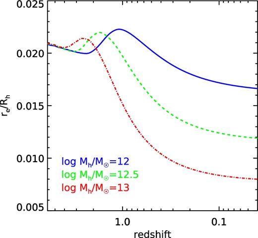
Examining the effect of star formation history on galaxy size. Using halo mass dependent star formation histories derived from abundance matching, we assume that new stars were formed in an exponential disc with a half-mass radius of 0.036 R_h(z), with the same centre and orientation as previous generations. At each redshift, we stack all stars formed (accounting for appropriate stellar mass loss) and compute the ratio of the stellar half-mass radius to R_h. For today's high-mass galaxies (10¹³M_⊙ haloes), there is quite a lot of evolution in this ratio, because most of the stars were formed early on when the halo was much smaller, and there is little late star formation. For lower mass galaxies (10¹²M_⊙ haloes), the effect is smaller, about 30 per cent. For even lower masses, we expect the effect to be even smaller.

Open in new tab Download slide

Perhaps the only way to reconcile the idea that disc sizes reflect the halo size at some earlier epoch with the results presented above would be if the gas stopped falling in to the disc at some point, and star formation continued as that disc gas reservoir was converted into stars. This probably happens to some extent. However, both numerical hydrodynamic simulations (Faucher-Giguère, Kereš & Ma 2011; Anglés-Alcázar et al. 2017) and observations of galaxy gas content and consumption times at z ∼ 1–2 (Saintonge et al. 2013; Genzel et al. 2015) are inconsistent with gas accretion ceasing completely at z ∼ 1–2 in disc galaxies in Milky Way or smaller sized haloes.

Desmond & Wechsler (2015) investigated a model based on abundance matching and an angular momentum partition model similar to equation (6), but allowing for expansion as well as contraction due to baryonic processes. They found that they were able to reproduce the normalization and slope of the z ∼ 0 mass–size relation with a value of f_j (in our notation) of 0.74–0.87, depending on the halo property used in the abundance matching.

5.4.2 Theoretical expectations for spheroid sizes

One of the surprising results of this work (already emphasized by K13) is that the linear proportionality r_e ∝ λR_h seems to work just as well for spheroid-dominated galaxies at z ∼ 0.1 as it does for discs – and in the nearby universe, the value of SRHR is almost the same for stellar mass bins that are mostly comprised of spheroid-dominated galaxies and those that are mostly comprised of disc-dominated galaxies. However, a new result shown in this work is that there are hints that SRHR has a stronger dependence on stellar mass at high redshift, such that SRHR is smaller for higher mass galaxies at high redshift. Why should SRHR be lower for high-mass galaxies at high redshift, but then converge to the same value as for lower mass galaxies by z ∼ 0.4?

This may be consistent with the picture in which massive galaxies at high redshift experience significant loss of angular momentum and compaction due to dissipational processes such as mergers and violent disc instabilities (Dekel & Burkert 2014; Porter et al. 2014a; Zolotov et al. 2015). Some of the gas that has been stripped of angular momentum is able to accrete on to a central supermassive black hole, which subsequently drives gas out of the galaxy with powerful winds and stops further cooling. The remnants are then ‘puffed up’ by dry (gas poor), mostly minor mergers (Naab, Johansson & Ostriker 2009; Shankar et al. 2010, 2013; Hilz, Naab & Ostriker 2013; Porter et al. 2014a,b). As the galaxy then acquires angular momentum from the orbits of the merged satellites, it is perhaps not so surprising after all that the angular momentum of the satellite population traces that of the host dark matter halo. We work these ideas out in more detail, and explore their implications for the size evolution of both discs and spheroids, in numerical hydrodynamic simulations (Choi et al. in preparation) and SAM (Somerville et al. in preparation).

5.4.3 Theoretical expectations for conditional size distributions

We found that the conditional distribution of P(λR_h|m_*) from our SHAM is in remarkable agreement with the observed conditional size distributions (size distribution in a bin of stellar mass and redshift, P(r_e|m_*)). We found this to be the case in both the GAMA and CANDELS samples in all redshift bins from 0.1 < z < 3. This point was already made in K13 with respect to nearby galaxies, but we have shown it here more explicitly, in greater detail, and also for a mass-selected high-redshift galaxy sample.

This result is surprising for several reasons. First, in the context of SAM of disc size such as equation (6) above, we expect additional dispersion to arise from the terms depending on disc mass (f_d) and halo concentration (c_NFW). Both of these quantities are expected to have significant halo-to-halo scatter. Indeed, Desmond & Wechsler (2015) showed that a model based on abundance matching plus an angular momentum partition type model similar to equation (6) produces too large a scatter in galaxy size at fixed stellar mass. Secondly, it holds across populations that are almost entirely disc dominated to ones that are almost entirely composed of giant ellipticals. This seems a non-trivial finding, given that discs are rotation supported while spheroids are supported by velocity dispersion. It may be a coincidence, or it may tell us something fundamental about the way that galaxies form. It may also appear surprising in view of the large (roughly two orders of magnitude) galaxy-to-galaxy scatter in the relationship between galaxy spin and halo spin (λ_galaxy versus λ_h) predicted by numerical simulations, as discussed in the introduction. However, we emphasize that these two findings are not necessarily inconsistent, although they do tell us something important about the physical processes that shape galaxy structure.

The ratio λ_galaxy/λ_h is equivalent to the ratio of the specific angular momenta of the galaxy and the DM halo (J_gal/M_gal)/(J_h/M_h) ≡ (j_gal/j_h), sometimes denoted f_j, and often adopted as a parameter in SAM. For a disc, we can write (adopting the Bullock definition of spin)

\begin{equation} r_{d} = f_j \,\, \left(\frac{V_{\rm h}}{V_{\rm rot}}\right) (\lambda _{{B}} R_{\rm h}), \end{equation}

(7)

where r_d is the exponential scale radius of the disc, V_h is the virial velocity of the halo, V_rot is the rotation velocity of the disc and other quantities are as defined previously. It is clear from this example that an anticorrelation between any of the terms (such as f_j and V_h/V_rot or f_j and λ_h, neither of which would be difficult to motivate physically) could reconcile a large dispersion in f_j with our results.

It is also entirely possible that the distributions of λ_galaxy and λ_h could be similar, even if their values are not well correlated for individual galaxies. This picture appears to be supported by the results of the Ceverino et al. (2014) numerical hydrodynamic simulations (Dekel et al. in preparation). This could arise if, for example, the values of λ_galaxy and λ_halo are determined by the physical conditions at different times, or different spatial locations. In addition, Burkert et al. (2016) found that the dispersion in galaxy spin parameter λ_galaxy for observed star-forming galaxies at redshift ∼0.8–2 is similar to the dispersion in halo spin parameters in dissipationless simulations. Investigating whether comparable distributions of λ_galaxy and λ_halo are indeed naturally and generically produced in numerical cosmological simulations, and better understanding the physical processes that lead to this result, is an important issue to follow up.

Although we have included a simplified estimate of errors in the stellar mass measurements in our SHAM, we have made no effort to deconvolve the observational errors in the size measurements or to add errors to the theoretical size predictions. The observational size distributions are of course broadened by both size and stellar mass measurement errors, implying that the theoretically predicted size distributions are actually somewhat broader than the intrinsic observed ones. However, it is also possible that the breadth of the observational distributions is underestimated due to selection effects. Galaxies with very large sizes may be missed due to surface brightness selection effects (or their sizes underestimated), and galaxies with very small sizes may be mistaken for stars, may be unresolved, or may be preferentially discarded because the fit quality is poor. One can see from Fig. 9 that the most compact galaxies predicted by the SHAM model are unresolved even by WFC3 on HST in the higher redshift bins, or contain only a few pixels.

Our results highlight the importance of confronting the observed conditional size distributions with predictions from state-of-the-art, high resolution numerical hydrodynamic simulations, including a detailed treatment of observational selection effects, errors and biases.

6 CONCLUSIONS

In this paper, we have explored an empirical approach for connecting (in a statistical sense) the observed radii of the stellar bodies of galaxies with the virial radii of their host dark matter haloes. We used a mapping between dark matter halo mass and stellar mass based on SHAM. We then explore observational constraints on the median relationship between galaxy effective radius and the halo virial radius (SRHR). In addition, we explore the median relationship between galaxy radius and the product of the halo spin parameter and the halo virial radius (SRHRλ). We find the following main results:

At z ∼ 0.1, the average ratio SRHR is consistent with being roughly independent of stellar mass, with a value of ∼0.018 over a broad range in stellar mass. Similarly, SRHRλ is nearly independent of stellar mass with a value of ∼0.5.
We find hints that SRHR and SRHRλ have a stronger dependence on stellar mass at high redshift than locally, with high-mass galaxies having a value of SRHR and SRHRλ that is about 50 per cent smaller than that of lower mass galaxies at z ∼ 2.
We find weak or negligible redshift evolution in SRHR over the interval 3 < z < 0.1. For galaxies with stellar mass |$m_* \lesssim 10^{10.3}{\,\,{\rm M}_{{\odot}}}$|⁠, SRHR has decreased by about a factor of 1.5 over this interval. For more massive galaxies, SRHR has increased by a similar factor from 3 < z < 0.4.
The preceding empirical results appear consistent with a picture in which massive galaxies at high redshift form via dissipative processes (such as gas-rich mergers or violent disc instabilities), leading to compact galaxies. As time progresses, galaxies become more gas poor, and massive galaxies seen closer to the present epoch are built up of a series of gas-poor mergers, leading to more extended stellar bodies.
The inferred redshift evolution of SRHRλ depends on the definition of the spin parameter that is adopted. If we adopt the Peebles definition of λ, we find a decrease of about a factor of 1.8 over 3 < z < 0.1 for galaxies with |$m_* \lesssim 10^{10.3}{\,\,{\rm M}_{{\odot}}}$|⁠, while if we use the Bullock definition of λ, we find results that are consistent with no significant change in SRHRλ over this time period.
We find the conditional distribution of λR_h in stellar mass bins from our SHAM is in remarkably good agreement with the observed conditional size distributions in stellar mass bins from z ∼ 0.1 to 3 (for both the GAMA and CANDELS samples). This suggests that there is little room for large galaxy-to-galaxy variations in SRHRλ, unless the width of the observed distribution is significantly underestimated, internal correlations conspire to reduce the dispersion, or galaxy size is uncorrelated with halo spin but by chance just happens to have a distribution with roughly the same width at fixed mass.
We caution that there are still significant uncertainties in key areas of this analysis, such as in converting from observed quantities (projected, light-weighted sizes) to intrinsic quantities (3D, stellar mass weighted sizes). These could impact our reported trends and further work is needed to constrain them better.

Our results provide guidelines for adding size information to SHAM-type models, as well as providing insights into the physics that shapes galaxy sizes over cosmic time.

Acknowledgements

We thank Seong-Kook Lee for helpful comments on the manuscript, and we thank Aldo Rodríguez-Puebla and Andrey Kravtsov for useful discussions. We thank Kuang-Han Huang for providing his data in electronic format and for helpful discussions. We thank the anonymous referee for comments and suggestions that improved the paper. We acknowledge the Kavli Institute for Theoretical Physics at the University of Santa Barbara, where part of this work was performed. This research was supported in part by the National Science Foundation under Grant No. NSF PHY-1125915. RSS thanks the Downsbrough family for their generous support, and acknowledges support from the Simons Foundation through a Simons Investigator grant. PB was supported by program number HST-HF2-51353.001-A, provided by NASA through a Hubble Fellowship grant from the Space Telescope Science Institute, which is operated by the Association of Universities for Research in Astronomy, Incorporated, under NASA contract NAS5-26555. PGP-G acknowledges support from Spanish MINECO Grants AYA2015-63650-P and AYA2015-70815-ERC. We acknowledge the contributions of hundreds of individuals to the planning and support of the CANDELS observations, and to the development and installation of new instruments on HST, without which this work would not have been possible. Support for HST Programs GO-12060 and GO-12099 was provided by NASA through grants from the Space Telescope Science Institute, which is operated by the Association of Universities for Research in Astronomy, Inc., under NASA contract NAS5-26555.

1

An alternative definition due to Bullock et al. (2001) is |$\lambda _{B} \equiv J(\sqrt{2} MVR)^{-1}$|⁠. Unless otherwise specified, λ denotes the Peebles definition in this work, but we also compare with the Bullock definition denoted by λ_B.

2

Both r_e and R_h need to be defined more carefully. We discuss this in later sections.

3

That is, the conversion from the size in one wavelength to that in another wavelength. We use this term in a general sense to also refer to the conversion from the half-light radius to the half stellar mass radius.

REFERENCES

Agertz

O.

,

Kravtsov

A. V.

,

2016

,

ApJ

,

824

,

79

Crossref

Search ADS

Anglés-Alcázar

D.

,

Faucher-Giguère

C.-A.

,

Kereš

D.

,

Hopkins

P. F.

,

Quataert

E.

,

Murray

N.

,

2017

,

MNRAS

,

470

,

4698

Crossref

Search ADS

Aumer

M.

,

White

S. D. M.

,

Naab

T.

,

2014

,

MNRAS

,

441

,

3679

Crossref

Search ADS

Barden

M.

et al. ,

2005

,

ApJ

,

635

,

959

Crossref

Search ADS

Behroozi

P. S.

,

Conroy

C.

,

Wechsler

R. H.

,

2010

,

ApJ

,

717

,

379

Crossref

Search ADS

Behroozi

P. S.

,

Wechsler

R. H.

,

Wu

H.-Y.

,

Busha

M. T.

,

Klypin

A. A.

,

Primack

J. R.

,

2013a

,

ApJ

,

763

,

18

Crossref

Search ADS

Behroozi

P. S.

,

Wechsler

R. H.

,

Conroy

C.

,

2013b

,

ApJ

,

770

,

57

Crossref

Search ADS

Benson

A. J.

,

2012

,

New Astron.

,

17

,

175

Crossref

Search ADS

Bernardi

M.

,

Shankar

F.

,

Hyde

J. B.

,

Mei

S.

,

Marulli

F.

,

Sheth

R. K.

,

2010

,

MNRAS

,

404

,

2087

Bernardi

M.

,

Meert

A.

,

Sheth

R. K.

,

Vikram

V.

,

Huertas-Company

M.

,

Mei

S.

,

Shankar

F.

,

2013

,

MNRAS

,

436

,

697

Crossref

Search ADS

Bernardi

M.

,

Meert

A.

,

Vikram

V.

,

Huertas-Company

M.

,

Mei

S.

,

Shankar

F.

,

Sheth

R. K.

,

2014

,

MNRAS

,

443

,

874

Crossref

Search ADS

Berry

M.

,

Somerville

R. S.

,

Haas

M. R.

,

Gawiser

E.

,

Maller

A.

,

Popping

G.

,

Trager

S. C.

,

2014

,

MNRAS

,

441

,

939

Crossref

Search ADS

Bigiel

F.

,

Blitz

L.

,

2012

,

ApJ

,

756

,

183

Crossref

Search ADS

Blumenthal

G.

,

Faber

S.

,

Flores

R.

,

Primack

J.

,

1986

,

ApJ

,

301

,

27

Crossref

Search ADS

Brennan

R.

et al. ,

2017

,

MNRAS

,

465

,

619

Crossref

Search ADS

Brook

C. B.

,

Stinson

G.

,

Gibson

B. K.

,

Roškar

R.

,

Wadsley

J.

,

Quinn

T.

,

2012

,

MNRAS

,

419

,

771

Crossref

Search ADS

Brooks

A. M.

,

Governato

F.

,

Quinn

T.

,

Brook

C. B.

,

Wadsley

J.

,

2009

,

ApJ

,

694

,

396

Crossref

Search ADS

Brooks

A. M.

et al. ,

2011

,

ApJ

,

728

,

51

Crossref

Search ADS

Bryan

G. L.

,

Norman

M. L.

,

1998

,

ApJ

,

495

,

80

Crossref

Search ADS

Bullock

J. S.

,

Dekel

A.

,

Kolatt

T. S.

,

Kravtsov

A. V.

,

Klypin

A. A.

,

Porciani

C.

,

Primack

J. R.

,

2001

,

ApJ

,

555

,

240

Crossref

Search ADS

Burkert

A.

et al. ,

2016

,

ApJ

,

826

,

214

Crossref

Search ADS

Busha

M. T.

,

Evrard

A. E.

,

Adams

F. C.

,

Wechsler

R. H.

,

2005

,

MNRAS

,

363

,

L11

Crossref

Search ADS

Cassata

P.

et al. ,

2011

,

ApJ

,

743

,

96

Crossref

Search ADS

Ceverino

D.

,

Klypin

A.

,

Klimek

E. S.

,

Trujillo-Gomez

S.

,

Churchill

C. W.

,

Primack

J.

,

Dekel

A.

,

2014

,

MNRAS

,

442

,

1545

Crossref

Search ADS

Ceverino

D.

,

Primack

J.

,

Dekel

A.

,

2015

,

MNRAS

,

453

,

408

Crossref

Search ADS

Chabrier

G.

,

2003

,

PASP

,

115

,

763

Crossref

Search ADS

Christensen

C.

,

Quinn

T.

,

Governato

F.

,

Stilp

A.

,

Shen

S.

,

Wadsley

J.

,

2012

,

MNRAS

,

425

,

3058

Crossref

Search ADS

Cole

S.

,

Lacey

C. G.

,

Baugh

C. M.

,

Frenk

C. S.

,

2000

,

MNRAS

,

319

,

168

Crossref

Search ADS

Conroy

C.

,

Wechsler

R. H.

,

Kravtsov

A. V.

,

2006

,

ApJ

,

647

,

201

Crossref

Search ADS

Courteau

S.

,

Dutton

A. A.

,

van den Bosch

F. C.

,

MacArthur

L. A.

,

Dekel

A.

,

McIntosh

D. H.

,

Dale

D. A.

,

2007

,

ApJ

,

671

,

203

Crossref

Search ADS

Covington

M.

,

Dekel

A.

,

Cox

T. J.

,

Jonsson

P.

,

Primack

J. R.

,

2008

,

MNRAS

,

384

,

94

Crossref

Search ADS

Crain

R. A.

et al. ,

2015

,

MNRAS

,

450

,

1937

Crossref

Search ADS

Croton

D. J.

et al. ,

2006

,

MNRAS

,

365

,

11

Crossref

Search ADS

Croton

D. J.

et al. ,

2016

,

ApJS

,

222

,

22

Crossref

Search ADS

Curtis-Lake

E.

et al. ,

2016

,

MNRAS

,

457

,

440

Crossref

Search ADS

Dahlen

T.

,

Mobasher

B.

,

Faber

S. M.

,

Ferguson

H. C.

,

Barro

G.

,

Finkelstein

S. L.

,

2013

,

ApJ

,

775

,

93

Crossref

Search ADS

Damjanov

I.

et al. ,

2011

,

ApJ

,

739

,

L44

Crossref

Search ADS

Danovich

M.

,

Dekel

A.

,

Hahn

O.

,

Ceverino

D.

,

Primack

J.

,

2015

,

MNRAS

,

449

,

2087

Crossref

Search ADS

de Jong

R. S.

,

Lacey

C.

,

2000

,

ApJ

,

545

,

781

Crossref

Search ADS

Dekel

A.

,

Burkert

A.

,

2014

,

MNRAS

,

438

,

1870

Crossref

Search ADS

Dekel

A.

,

Cox

T. J.

,

2006

,

MNRAS

,

370

,

1445

Crossref

Search ADS

Dekel

A.

,

Sari

R.

,

Ceverino

D.

,

2009

,

ApJ

,

703

,

785

Crossref

Search ADS

Dekel

A.

,

Zolotov

A.

,

Tweed

D.

,

Cacciato

M.

,

Ceverino

D.

,

Primack

J. R.

,

2013

,

MNRAS

,

435

,

999

Crossref

Search ADS

Desmond

H.

,

Wechsler

R. H.

,

2015

,

MNRAS

,

454

,

322

Crossref

Search ADS

Desmond

H.

,

Mao

Y.-Y.

,

Wechsler

R.

,

Crain

R.

,

Schaye

J.

,

2017

,

MNRAS

,

471

,

11

Diemer

B.

,

More

S.

,

Kravtsov

A. V.

,

2013

,

ApJ

,

766

,

25

Crossref

Search ADS

Driver

S. P.

et al. ,

2011

,

MNRAS

,

413

,

971

Crossref

Search ADS

Dutton

A. A.

,

van den Bosch

F. C.

,

2012

,

MNRAS

,

421

,

608

Dutton

A. A.

,

van den Bosch

F. C.

,

Dekel

A.

,

Courteau

S.

,

2007

,

ApJ

,

654

,

27

Crossref

Search ADS

Dutton

A. A.

et al. ,

2011a

,

MNRAS

,

410

,

1660

Dutton

A. A.

et al. ,

2011b

,

MNRAS

,

416

,

322

Faucher-Giguère

C.-A.

,

Kereš

D.

,

Ma

C.-P.

,

2011

,

MNRAS

,

417

,

2982

Crossref

Search ADS

Ferguson

H. C.

et al. ,

2004

,

ApJ

,

600

,

L107

Crossref

Search ADS

Flores

R.

,

Primack

J.

,

Blumenthal

G.

,

Faber

S.

,

1993

,

ApJ

,

412

,

443

Crossref

Search ADS

Furlong

M.

et al. ,

2017

,

MNRAS

,

465

,

722

Galametz

A.

et al. ,

2013

,

ApJS

,

206

,

10

Crossref

Search ADS

Genel

S.

,

Fall

S. M.

,

Hernquist

L.

,

Vogelsberger

M.

,

Snyder

G. F.

,

Rodriguez-Gomez

V.

,

Sijacki

D.

,

Springel

V.

,

2015

,

ApJ

,

804

,

L40

Crossref

Search ADS

Genzel

R.

et al. ,

2015

,

ApJ

,

800

,

20

Crossref

Search ADS

Giavalisco

M.

,

Steidel

C.

,

Macchetto

D.

,

1996

,

ApJ

,

470

,

189

Crossref

Search ADS

Governato

F.

et al. ,

2004

,

ApJ

,

607

,

688

Crossref

Search ADS

Governato

F.

,

Willman

B.

,

Mayer

L.

,

Brooks

A.

,

Stinson

G.

,

Valenzuela

O.

,

Wadsley

J.

,

Quinn

T.

,

2007

,

MNRAS

,

374

,

1479

Crossref

Search ADS

Grogin

N. A.

et al. ,

2011

,

ApJS

,

197

,

35

Crossref

Search ADS

Guedes

J.

,

Callegari

S.

,

Madau

P.

,

Mayer

L.

,

2011

,

ApJ

,

742

,

76

Crossref

Search ADS

Guo

Q.

,

White

S.

,

Li

C.

,

Boylan-Kolchin

M.

,

2010

,

MNRAS

,

404

,

1111

Guo

Y.

et al. ,

2013

,

ApJS

,

207

,

24

Crossref

Search ADS

Henriques

B. M. B.

,

White

S. D. M.

,

Thomas

P. A.

,

Angulo

R.

,

Guo

Q.

,

Lemson

G.

,

Springel

V.

,

Overzier

R.

,

2015

,

MNRAS

,

451

,

2663

Crossref

Search ADS

Hernquist

L.

,

Mihos

J. C.

,

1995

,

ApJ

,

448

,

41

Crossref

Search ADS

Hilz

M.

,

Naab

T.

,

Ostriker

J. P.

,

2013

,

MNRAS

,

429

,

2924

Crossref

Search ADS

Hopkins

P. F.

,

Cox

T. J.

,

Younger

J. D.

,

Hernquist

L.

,

2009

,

ApJ

,

691

,

1168

Crossref

Search ADS

Huang

K.-H.

,

Ferguson

H. C.

,

Ravindranath

S.

,

Su

J.

,

2013

,

ApJ

,

765

,

68

Crossref

Search ADS

Huang

K.

et al. ,

2017

,

ApJ

,

838

,

6

Kauffmann

G.

,

1996

,

MNRAS

,

281

,

475

Crossref

Search ADS

Kawamata

R.

,

Ishigaki

M.

,

Shimasaku

K.

,

Oguri

M.

,

Ouchi

M.

,

2015

,

ApJ

,

804

,

103

Crossref

Search ADS

Kelvin

L. S.

et al. ,

2012

,

MNRAS

,

421

,

1007

Crossref

Search ADS

Klypin

A. A.

,

Trujillo-Gomez

S.

,

Primack

J.

,

2011

,

ApJ

,

740

,

102

Crossref

Search ADS

Knebe

A.

et al. ,

2011

,

MNRAS

,

415

,

2293

Crossref

Search ADS

Koekemoer

A. M.

et al. ,

2011

,

ApJS

,

197

,

36

Crossref

Search ADS

Kormendy

J.

,

1977

,

ApJ

,

218

,

333

Crossref

Search ADS

Kravtsov

A. V.

,

2013

,

ApJ

,

764

,

L31

(K13)

Crossref

Search ADS

Kravtsov

A.

,

Vikhlinin

A.

,

Meshscheryakov

A.

,

2014

,

preprint (arXiv:1401.7329)

Lacey

C. G.

et al. ,

2016

,

MNRAS

,

462

,

3854

Crossref

Search ADS

Lange

R.

et al. ,

2015

,

MNRAS

,

447

,

2603

Crossref

Search ADS

Lilly

S.

et al. ,

1998

,

ApJ

,

500

,

75

Crossref

Search ADS

Liske

J.

et al. ,

2015

,

MNRAS

,

452

,

2087

Crossref

Search ADS

Lowenthal

J.

et al. ,

1997

,

ApJ

,

481

,

673

Crossref

Search ADS

Mo

H.

,

Mao

S.

,

White

S.

,

1998

,

MNRAS

,

295

,

319

Crossref

Search ADS

Mobasher

B.

et al. ,

2015

,

ApJ

,

808

,

101

Crossref

Search ADS

Momcheva

I. G.

et al. ,

2016

,

ApJS

,

225

,

27

Crossref

Search ADS

Monaco

P.

,

Fontanot

F.

,

Taffoni

G.

,

2007

,

MNRAS

,

375

,

1189

Crossref

Search ADS

Moster

B. P.

,

Somerville

R. S.

,

Maulbetsch

C.

,

van den Bosch

F. C.

,

Macciò

A. V.

,

Naab

T.

,

Oser

L.

,

2010

,

ApJ

,

710

,

903

Crossref

Search ADS

Moster

B. P.

,

Naab

T.

,

White

S. D. M.

,

2013

,

MNRAS

,

428

,

3121

Crossref

Search ADS

Munshi

F.

et al. ,

2013

,

ApJ

,

766

,

56

Crossref

Search ADS

Naab

T.

,

Johansson

P. H.

,

Ostriker

J. P.

,

2009

,

ApJ

,

699

,

178

Crossref

Search ADS

Navarro

J. F.

,

Steinmetz

M.

,

2000

,

ApJ

,

538

,

477

Crossref

Search ADS

Navarro

J. F.

,

Frenk

C. S.

,

White

S. D. M.

,

1997

,

ApJ

,

490

,

493

Crossref

Search ADS

Nayyeri

H.

et al. ,

2017

,

ApJS

,

228

,

7

Crossref

Search ADS

Newman

A. B.

,

Ellis

R. S.

,

Treu

T.

,

Bundy

K.

,

2010

,

ApJ

,

717

,

L103

Crossref

Search ADS

Oesch

P. A.

et al. ,

2010

,

ApJ

,

709

,

L21

Crossref

Search ADS

Peebles

P. J. E.

,

1969

,

ApJ

,

155

,

393

Crossref

Search ADS

Peng

C. Y.

,

Ho

L. C.

,

Impey

C. D.

,

Rix

H.-W.

,

2002

,

AJ

,

124

,

266

Crossref

Search ADS

Planck Collaboration XVI

,

2014

,

A&A

,

571

,

A16

Crossref

Search ADS

Popping

G.

,

Somerville

R. S.

,

Trager

S. C.

,

2014

,

MNRAS

,

442

,

2398

Crossref

Search ADS

Porciani

C.

,

Dekel

A.

,

Hoffman

Y.

,

2002

,

MNRAS

,

332

,

325

Crossref

Search ADS

Porter

L. A.

,

Somerville

R. S.

,

Primack

J. R.

,

Johansson

P. H.

,

2014a

,

MNRAS

,

444

,

942

Crossref

Search ADS

Porter

L. A.

,

Somerville

R. S.

,

Primack

J. R.

,

Croton

D. J.

,

Covington

M. D.

,

Graves

G. J.

,

Faber

S. M.

,

2014b

,

MNRAS

,

445

,

3092

Crossref

Search ADS

Prugniel

P.

,

Simien

F.

,

1997

,

A&A

,

321

,

111

Ravindranath

S.

et al. ,

2004

,

ApJ

,

604

,

L9

Crossref

Search ADS

Rodríguez-Puebla

A.

,

Avila-Reese

V.

,

Yang

X.

,

Foucaud

S.

,

Drory

N.

,

Jing

Y. P.

,

2015

,

ApJ

,

799

,

130

Crossref

Search ADS

Rodríguez-Puebla

A.

,

Primack

J. R.

,

Behroozi

P.

,

Faber

S. M.

,

2016a

,

MNRAS

,

455

,

2592

Crossref

Search ADS

Rodríguez-Puebla

A.

,

Behroozi

P.

,

Primack

J.

,

Klypin

A.

,

Lee

C.

,

Hellinger

D.

,

2016b

,

MNRAS

,

462

,

893

Crossref

Search ADS

Rodriguez-Puebla

A.

,

Primack

J. R.

,

Avila-Reese

V.

,

Faber

S. M.

,

2017

,

MNRAS

,

470

,

651

Saintonge

A.

et al. ,

2013

,

ApJ

,

778

,

2

(RP17)

Crossref

Search ADS

Sales

L. V.

,

Navarro

J. F.

,

Schaye

J.

,

Dalla Vecchia

C.

,

Springel

V.

,

Haas

M. R.

,

Helmi

A.

,

2009

,

MNRAS

,

399

,

L64

Crossref

Search ADS

Santini

P.

et al. ,

2015

,

ApJ

,

801

,

97

Crossref

Search ADS

Scannapieco

C.

et al. ,

2012

,

MNRAS

,

423

,

1726

Crossref

Search ADS

Schaye

J.

et al. ,

2015

,

MNRAS

,

446

,

521

Crossref

Search ADS

Shankar

F.

,

Marulli

F.

,

Bernardi

M.

,

Dai

X.

,

Hyde

J. B.

,

Sheth

R. K.

,

2010

,

MNRAS

,

403

,

117

Crossref

Search ADS

Shankar

F.

,

Marulli

F.

,

Bernardi

M.

,

Mei

S.

,

Meert

A.

,

Vikram

V.

,

2013

,

MNRAS

,

428

,

109

Crossref

Search ADS

Shen

S.

et al. ,

2003

,

MNRAS

,

343

,

978

Crossref

Search ADS

Shibuya

T.

,

Ouchi

M.

,

Harikane

Y.

,

2015

,

ApJS

,

219

,

15

Crossref

Search ADS

Simard

L.

et al. ,

1999

,

ApJ

,

519

,

563

Crossref

Search ADS

Skelton

R. E.

et al. ,

2014

,

ApJS

,

214

,

24

Crossref

Search ADS

Snyder

G. F.

et al. ,

2015

,

MNRAS

,

454

,

1886

Crossref

Search ADS

Somerville

R. S.

,

Primack

J. R.

,

1999

,

MNRAS

,

310

,

1087

Crossref

Search ADS

Somerville

R. S.

,

Hopkins

P. F.

,

Cox

T. J.

,

Robertson

B. E.

,

Hernquist

L.

,

2008a

,

MNRAS

,

391

,

481

Crossref

Search ADS

Somerville

R. S.

et al. ,

2008b

,

ApJ

,

672

,

776

Crossref

Search ADS

Somerville

R. S.

,

Popping

G.

,

Trager

S. C.

,

2015

,

MNRAS

,

453

,

4337

Crossref

Search ADS

Sommer-Larsen

J.

,

Gelato

S.

,

Vedel

H.

,

1999

,

ApJ

,

519

,

501

Crossref

Search ADS

Speagle

J. S.

,

Steinhardt

C. L.

,

Capak

P. L.

,

Silverman

J. D.

,

2014

,

ApJS

,

214

,

15

Crossref

Search ADS

Stefanon

M.

et al. ,

2017

,

ApJS

,

229

,

32

Crossref

Search ADS

Steinmetz

M.

,

Navarro

J. F.

,

2002

,

New Astron.

,

7

,

155

Crossref

Search ADS

Stevens

A. R. H.

,

Lagos

C. d. P.

,

Contreras

S.

,

Croton

D. J.

,

Padilla

N. D.

,

Schaller

M.

,

Schaye

J.

,

Theuns

T.

,

2017

,

MNRAS

,

467

,

2066

Stewart

K. R.

,

Brooks

A. M.

,

Bullock

J. S.

,

Maller

A. H.

,

Diemand

J.

,

Wadsley

J.

,

Moustakas

L. A.

,

2013

,

ApJ

,

769

,

74

Crossref

Search ADS

Szomoru

D.

,

Franx

M.

,

van Dokkum

P. G.

,

Trenti

M.

,

Illingworth

G. D.

,

Labbé

I.

,

Oesch

P.

,

2013

,

ApJ

,

763

,

73

Crossref

Search ADS

Taylor

E. N.

et al. ,

2011

,

MNRAS

,

418

,

1587

Crossref

Search ADS

Teklu

A. F.

,

Remus

R.-S.

,

Dolag

K.

,

Beck

A. M.

,

Burkert

A.

,

Schmidt

A. S.

,

Schulze

F.

,

Steinborn

L. K.

,

2015

,

ApJ

,

812

,

29

Crossref

Search ADS

Tinker

J. L.

et al. ,

2017

,

ApJ

,

839

,

121

Crossref

Search ADS

Trujillo

I.

et al. ,

2006

,

ApJ

,

650

,

18

Crossref

Search ADS

Übler

H.

,

Naab

T.

,

Oser

L.

,

Aumer

M.

,

Sales

L. V.

,

White

S. D. M.

,

2014

,

MNRAS

,

443

,

2092

Crossref

Search ADS

van der Wel

A.

,

Bell

E. F.

,

van den Bosch

F. C.

,

Gallazzi

A.

,

Rix

H.-W.

,

2009

,

ApJ

,

698

,

1232

Crossref

Search ADS

van der Wel

A.

et al. ,

2012

,

ApJS

,

203

,

24

Crossref

Search ADS

van der Wel

A.

et al. ,

2014a

,

ApJ

,

788

,

28

(vdW14)

Crossref

Search ADS

van der Wel

A.

et al. ,

2014b

,

ApJ

,

792

,

L6

Crossref

Search ADS

van Dokkum

P. G.

et al. ,

2008

,

ApJ

,

677

,

L5

Crossref

Search ADS

van Dokkum

P. G.

et al. ,

2015

,

ApJ

,

813

,

23

Crossref

Search ADS

Vitvitska

M.

,

Klypin

A. A.

,

Kravtsov

A. V.

,

Wechsler

R. H.

,

Primack

J. R.

,

Bullock

J. S.

,

2002

,

ApJ

,

581

,

799

Crossref

Search ADS

Vogelsberger

M.

et al. ,

2014

,

MNRAS

,

444

,

1518

Crossref

Search ADS

Wetzel

A. R.

,

Nagai

D.

,

2015

,

ApJ

,

808

,

40

Crossref

Search ADS

White

S. D. M.

,

1984

,

ApJ

,

286

,

38

Crossref

Search ADS

Wuyts

S.

et al. ,

2011

,

ApJ

,

742

,

96

Crossref

Search ADS

Wuyts

S.

et al. ,

2012

,

ApJ

,

753

,

114

Crossref

Search ADS

Zavala

J.

et al. ,

2016

,

MNRAS

,

460

,

4466

Crossref

Search ADS

Zheng

Z.

et al. ,

2005

,

ApJ

,

633

,

791

Crossref

Search ADS

Zjupa

J.

,

Springel

V.

,

2017

,

MNRAS

,

466

,

1625

Crossref

Search ADS

Zolotov

A.

et al. ,

2015

,

MNRAS

,

450

,

2327

Crossref

Search ADS

APPENDIX A: OBSERVED SIZE–MASS RELATIONS

In Fig. A1, we show the size–mass relation for the GAMA sample that we use in this work. We show the relation for galaxies with Sérsic index n_s < 2.5 (disc-dominated galaxies) and n_s > 2.5 (spheroid-dominated galaxies) separately, as we apply corrections for deprojection and to convert from half-light radii to half stellar mass radii based on this division. We show a comparison between the mean and median sizes in stellar mass bins from our analysis and several relations from the literature, including the analysis of GAMA by Lange et al. (2015) and the analysis of SDSS by Bernardi et al. (2014). The GAMA sizes appear to be systematically larger at a given stellar mass than the SDSS sizes. Note that the Bernardi et al. (2014) sizes are circularized, while the GAMA-based sizes in our analysis and that of Lange et al. (2015) are semimajor axis sizes. By comparing the Bernardi et al. (2014) results with the circularized size measurements from the GAMA data base, it can be shown that this difference largely explains the offset (Kravtsov, private communication).

Figure A1.

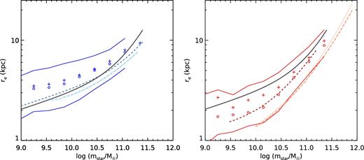
Observed size–mass relation for the GAMA sample used in this analysis, compared with other relations from the literature. Here, r_e is the semimajor axis half-light radius in the r band. Left-hand panel: relation for disc-like galaxies with Sérsic parameter n_s < 2.5. Crosses show means, while open circles show medians. Solid blue lines show the 16th and 84th percentiles. The grey-blue dashed line shows the fitting function for n_s < 2.5 galaxies given in Lange et al. (2015), and light blue dotted and dot–dashed lines show the results for single Sérsic and Sérsic+exponential fits (respectively) from Bernardi et al. (2014). Note that the Bernardi et al. (2014) sizes are circularized. Right-hand panel: relation for spheroid-dominated galaxies with Sérsic parameter n_s > 2.5. Lines and symbols are as in the left-hand panel, but all for n_s > 2.5 galaxies. The dark grey solid line in both panels shows the size–mass relation for the disc- and spheroid-dominated samples combined, converted to the 3D stellar half-mass radius using the type-dependent correction described in the text.

Open in new tab Download slide

In Fig. A2, we show our derived size–mass relations for the CANDELS sample used in this work. Here, we show the full sample, without dividing into different galaxy types, but we again apply a Sérsic-dependent correction for deprojection and to convert from light to stellar mass. Our derived size–mass relation is in excellent agreement with the published results of vdW14 and H17.

Figure A2.

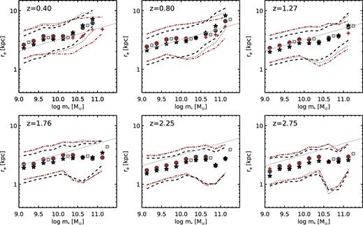
Observed size–mass relation for the CANDELS sample used in this work, in redshift bins as indicated on the panels. Dark-grey filled circles: results from our analysis. Open squares: results from the published analysis of vdW14. Red crosses: results from the analysis of H17. All of the preceding show median rest 5000 Å half-light radii. The light grey line, repeated in each panel, shows the size–mass relation from the z = 0.1 GAMA sample. There is good agreement between the observed size–mass relation published by van der Wel et al. (2014a), that derived from our analysis of the CANDELS team catalogues, and that derived from the analysis of H17. Black stars: estimated median 3D stellar half-mass radii obtained by applying the type-dependent corrections described in the text to the CANDELS sample.

Open in new tab Download slide

APPENDIX B: HALO STRUCTURAL PARAMETER DEFINITIONS

In this appendix, we show the differences between different definitions of halo virial radius and spin parameter. It has become customary to define dark matter haloes as spherical overdensities within which the average overdensity exceeds a threshold value. However, different values of this overdensity parameter are used in the literature. The most common conventions are to assume a fixed overdensity of 200 or to assume a redshift-dependent overdensity Δ_vir as given in Bryan & Norman (1998). To make matters even more confusing, some studies apply the overdensity threshold relative to the critical density of the Universe while others use the background density. This results in different values of R_h for a given M_h, different values of halo number density (or abundance) at a given M_h, and different redshift evolution for all quantities. It also results in different values for the total angular momentum of the halo, J_h, and spin parameter λ.

In Fig. B1, we show the virial radius as a function of redshift for a halo with a mass of |$10^{12}{\,\,{\rm M}_{{\odot}}}$|⁠. We also show the virial radius as a function of redshift at fixed mass, normalized to the value at z = 0. One can see from this figure that the halo radius at a given mass differs at z = 0 by as much as a factor of 2 in different definitions, while all definitions produce nearly the same value above z ∼ 3. As a result, conclusions about the evolution of halo radius across cosmic time can also differ by a similar factor. The ‘200 crit’ definition produces the least evolution, while the ‘vir background’ definition produces the most.

Figure B1.

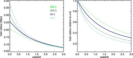
Halo radius versus redshift for different definitions of halo mass and radius. Solid dark blue: r_vir,crit; light blue dot–dashed: r_vir,b; green dotted: r_200,crit; dark green dashed: r_200,b (see text for definitions). Different definitions produce similar results at high redshift, but the halo radius may differ by as much as a factor of almost 2 in normalization at z = 0 for different definitions, and the inferred evolution can differ by a similar amount.

Open in new tab Download slide

The halo spin parameter clearly depends on the halo mass and radius definition. In addition, two different dimensionless spin parameters have been proposed in the literature, the ‘Peebles’ and ‘Bullock’ definitions described in Section 1. These are generally assumed to be interchangeable. In Fig. B2, we show the distributions of halo spin parameters in the Bolshoi–Planck simulations, in the six redshift bins used in the rest of our analysis (0.1–0.5, 0.5–1.0, 1.0–1.5, 1.5–2.0, 2.0–2.5 and 2.5–3.0; the redshift labels on the plots indicate the volume mid-point of each bin). We show the distributions for both the Peebles and Bullock definition of the halo spin parameter. In both Figs B2 and B3, we show only ‘distinct’ haloes (haloes that are not a sub-halo of another halo) with |$M_{h} > 10^{10.35}\,\,{\,\,{\rm M}_{{\odot}}}$| (this is the mass limit quoted by Rodríguez-Puebla et al. (2016b) for robust determination of halo structural properties in the Bolshoi–Planck simulations).

Figure B2.

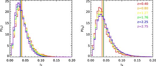
Distributions of the spin parameter λ in the Bolshoi–Planck simulations, in the redshift bins used in our analysis. Left: Peebles definition λ_P. Right: Bullock definition λ_B. Vertical lines show the medians in each redshift bin. The median value of λ_P, along with the whole distribution, shifts to larger values with decreasing redshift, while the median value and distribution of λ_B shift to smaller values with decreasing redshift.

Open in new tab Download slide

Figure B3.

Left: Median NFW concentration parameter versus halo mass for the same redshift bins used in our analysis. The shaded red area shows the 16 and 84th percentiles for the z = 0.1–0.5 bin. As is well known, halo concentrations at a fixed mass are lower at high redshift. Right: Ratio between the Peebles and Bullock definitions of the spin parameter in the Bolshoi–Planck halo catalogues as a function of the NFW concentration parameter. For perfect spherical haloes with no sub-structure, with all particles on circular orbits, λ_P/λ_B should be equal to the function (f_c)^1/2 (see text). The evolution of halo concentrations go in the right direction to explain the differing evolution of λ_P and λ_B in the simulations, but do not appear to provide a complete explanation, as seen from the evolution in λ_P/λ_B at fixed c_NFW.

Open in new tab Download slide

We see that the distribution of λ_P shifts towards larger values at lower redshift, while the distribution of λ_B shifts towards smaller values at lower redshift. The ratio of the median value of λ_P in the 2.5 < z < 3.0 bin to that in the 0.1 < z < 0.5 bin is 0.85, while this ratio is 1.16 for λ_B.

The original motivation behind the Peebles definition of the spin parameter λ_P was to represent the fraction of the total energy of a system in the form of ordered rotational motion. Thus, the total energy E comes in to the expression. In the special case of a truncated singular isothermal sphere in which all particles are on circular orbits,

\begin{equation} E = -\frac{GM^2}{2R} = -\frac{MV_{c}^2}{2}. \end{equation}

(B1)

Thus, we see that for truncated singular isothermal spheres with all particles on circular orbits, the Peebles and Bullock definitions of spin are the same (λ_P = λ_B). For the more cosmologically relevant (but still simplified) case of perfect NFW spheres with all particles on circular orbits, the total energy E is

\begin{equation} E = -\frac{GM^2}{2R} f_{c}, \end{equation}

(B2)

where the function f_c depends only on the NFW concentration parameter (see e.g. equation 23 of Mo et al. 1998). This function can be well-approximated by the fitting function (Mo et al. 1998)

\begin{equation} f_{c} \simeq \frac{2}{3} + \left(\frac{c_{\rm NFW}}{21.5}\right)^{0.7}. \end{equation}

(B3)

Thus, for smooth, spherical NFW haloes with all particles on circular orbits, λ_P/λ_B = (f_c)^1/2.

Fig. B3 shows the median halo mass versus NFW concentration parameter for haloes in the Bolshoi–Planck catalogues in the same redshift bins. As is well known, the concentration for a fixed halo mass is lower at high redshift. As f_c is a monotonically increasing function of the concentration parameter c_NFW, we would therefore expect λ_P/λ_B to be lower at high redshift as well (for fixed halo mass). However, we see from the right panel of Fig. B3 that the explanation appears to be somewhat more complicated: haloes have lower median values of λ_P/λ_B at high redshift even at fixed concentration. This could be due to haloes in cosmological simulations deviating from sphericity, having sub-structure, or deviating from having all particles on circular orbits, by different amounts at different redshifts. Clearly, this is an interesting issue to investigate in more detail, as it may have important implications for the structural properties of galaxies and their evolution.

Download all slides

Month:	Total Views:
September 2017	4
November 2017	11
December 2017	26
January 2018	30
February 2018	22
March 2018	22
April 2018	15
May 2018	21
June 2018	16
July 2018	16
August 2018	25
September 2018	13
October 2018	39
November 2018	34
December 2018	29
January 2019	22
February 2019	25
March 2019	34
April 2019	20
May 2019	20
June 2019	19
July 2019	20
August 2019	20
September 2019	36
October 2019	44
November 2019	26
December 2019	25
January 2020	31
February 2020	41
March 2020	19
April 2020	16
May 2020	18
June 2020	36
July 2020	57
August 2020	30
September 2020	60
October 2020	29
November 2020	58
December 2020	28
January 2021	37
February 2021	33
March 2021	30
April 2021	39
May 2021	35
June 2021	48
July 2021	32
August 2021	41
September 2021	36
October 2021	48
November 2021	44
December 2021	47
January 2022	47
February 2022	60
March 2022	63
April 2022	50
May 2022	56
June 2022	63
July 2022	38
August 2022	79
September 2022	70
October 2022	92
November 2022	68
December 2022	59
January 2023	39
February 2023	61
March 2023	49
April 2023	50
May 2023	53
June 2023	30
July 2023	43
August 2023	24
September 2023	21
October 2023	32
November 2023	39
December 2023	57
January 2024	43
February 2024	46
March 2024	41
April 2024	62
May 2024	79
June 2024	48
July 2024	38
August 2024	50
September 2024	71
October 2024	119
November 2024	76
December 2024	55
January 2025	62
February 2025	49
March 2025	50
April 2025	51
May 2025	56

Article Contents

The relationship between galaxy and dark matter halo size from z ∼ 3 to the present

Abstract

1 INTRODUCTION

2 MODELS AND METHODS

2.1 Simulations and dark matter haloes

2.2 Relating (sub-)haloes to galaxies

3 OBSERVATIONAL DATA

3.1 GAMA

3.2 CANDELS

3.3 Converting from projected light to 3D stellar mass sizes

4 RESULTS

4.1 Results from the GAMA survey at z = 0.1

4.2 Results from the CANDELS survey at 0.1 < z < 3.0

5 DISCUSSION

5.1 Main caveats and uncertainties

5.1.1 Halo properties and SMHM relation

5.1.2 Definition of halo spin parameter

5.1.3 Observational measurements

5.2 Beware backwards modelling

5.3 Comparison with previous work

5.4 Physical interpretation

5.4.1 Theoretical expectations for disc sizes

5.4.2 Theoretical expectations for spheroid sizes

5.4.3 Theoretical expectations for conditional size distributions

6 CONCLUSIONS

Acknowledgements

REFERENCES

APPENDIX A: OBSERVED SIZE–MASS RELATIONS

APPENDIX B: HALO STRUCTURAL PARAMETER DEFINITIONS

Citations

Views

Altmetric

Email alerts

Astrophysics Data System

Citing articles via

Latest

Most Read

Most Cited

Article Contents

The relationship between galaxy and dark matter halo size from z ∼ 3 to the present Free

Abstract

1 INTRODUCTION

2 MODELS AND METHODS

2.1 Simulations and dark matter haloes

2.2 Relating (sub-)haloes to galaxies

3 OBSERVATIONAL DATA

3.1 GAMA

3.2 CANDELS

3.3 Converting from projected light to 3D stellar mass sizes

4 RESULTS

4.1 Results from the GAMA survey at z = 0.1

4.2 Results from the CANDELS survey at 0.1 < z < 3.0

5 DISCUSSION

5.1 Main caveats and uncertainties

5.1.1 Halo properties and SMHM relation

5.1.2 Definition of halo spin parameter

5.1.3 Observational measurements

5.2 Beware backwards modelling

5.3 Comparison with previous work

5.4 Physical interpretation

5.4.1 Theoretical expectations for disc sizes

5.4.2 Theoretical expectations for spheroid sizes

5.4.3 Theoretical expectations for conditional size distributions

6 CONCLUSIONS

Acknowledgements

REFERENCES

APPENDIX A: OBSERVED SIZE–MASS RELATIONS

APPENDIX B: HALO STRUCTURAL PARAMETER DEFINITIONS

Citations

Views

Altmetric

Email alerts

Astrophysics Data System

Citing articles via

Latest

Most Read

Most Cited

This Feature Is Available To Subscribers Only

The relationship between galaxy and dark matter halo size from z ∼ 3 to the present