


Abstract
We estimate the stellar mass that satellite galaxies lose once they enter groups (and clusters) by identifying groups in a high-resolution cosmological N-body simulation, assigning entry masses to satellite galaxies with halo abundance matching at the entry time and comparing the predicted conditional stellar mass function of satellite galaxies at z ≃ 0 with observations. Our results depend on the mass of the stars that form in satellite galaxies after the entry time. A model in which star formation shuts down completely as soon a galaxy enters a group environment is ruled out because it underpredicts the stellar masses of satellite galaxies even in the absence of tidal stripping. The greater is the stellar mass that can form, the greater the fraction that needs to be tidally stripped. The stellar mass fraction lost by satellite galaxies after entering a group or cluster environment is consistent with any value in the range 0–40 per cent. To place stronger constraints, we consider a more refined model of tidal stripping of galaxies on elongated orbits (where stripping occurs at orbit pericentres). Our model predicts less tidal stripping: satellite galaxies lose ∼20–25 per cent of their stellar mass since their entry into the group. This finding is consistent with a slow-starvation delayed-quenching picture, in which galaxies that enter a group or cluster environment keep forming stars until at least the first pericentric passage.
1 INTRODUCTION
1.1 Constraints from the intracluster light
The notion of intracluster light (ICL) began to emerge after Zwicky (1957) and Welch & Sastry (1971) detected a diffuse luminous background around NCG 4874 and NGC 4889, the two supergiant elliptical galaxies that dominate the central region of the Coma cluster. Since central dominant (cD) galaxies with extensive outer envelopes are a common occurrence in very rich clusters (Matthews, Morgan & Schmidt 1964; Morgan & Lesh 1965; Bautz & Morgan 1970), Gallagher & Ostriker (1972) interpreted the ICL at the centre of Coma as ‘a diffuse intergalactic cloud of stars evaporated from colliding galaxies’, which ‘will contribute to the formation of a cD system's envelope or in fact may constitute the cD “galaxy” itself’. Analytical calculations and N-body simulations have confirmed that tidal stripping by companion galaxies and by the cluster's potential can explain the origin of the ICL (e.g. Merritt 1983; Mamon 1987; Ghigna et al. 1998; Hayashi et al. 2003; Willman et al. 2004; Mihos et al. 2005; Abadi, Navarro & Steinmetz 2006; Purcell, Bullock & Zentner 2007). Klimentowski et al. (2009), Łokas, Kazantzidis & Mayer (2011) and Kazantzidis et al. (2011) found a median stellar mass loss of ∼30–35 per cent at each pericentric passage.
Forty years after Gallagher & Ostriker (1972), there is still no consensus whether the outer envelopes of cD galaxies belong to the ICL or to the galaxies themselves. The issue could be dismissed as largely semantic, but is also the reason why the galaxy stellar mass functions (SMFs) of Baldry et al. (2012) and Bernardi et al. (2013) differ by ∼0.5 dex at high masses (but see Bernardi et al. 2017).
The ICL contributes ∼10–30 per cent of a cluster's total luminosity (Gonzalez, Zabludoff & Zaritsky 2005; Zibetti et al. 2005; Krick, Bernstein & Pimbblet 2006) and sometimes even more (Lin & Mohr 2004). However, stellar haloes formed out of disrupted satellites are also present in lower mass systems. In particular, it has become clear that the stellar halo of the Milky Way contains considerable substructure in the form of stellar streams (Helmi et al. 1999; Yanny et al. 2003; Bell et al. 2008). In some cases, the streams can be unambiguously associated with the satellite galaxies from which they came (Ibata, Gilmore & Irwin 1994; Odenkirchen et al. 2002). Similar streams have also been detected in our neighbour galaxy M31 (e.g. Ferguson et al. 2002). In this article, we assess the impact of tidal stripping on the stellar masses of galaxies not just in clusters but across a broad range of environments.
1.2 Constraints from the growth of cD galaxies
Conroy, Wechsler & Kravtsov (2007) studied the mass growth of cD galaxies from z ∼ 1 to 0 by using the abundance matching (AM) technique (Marinoni & Hudson 2002; Vale & Ostriker 2004), described in detail by Behroozi, Conroy & Wechsler (2010), which assumes that halo masses (or equivalent properties) are strongly correlated with observable galaxy properties such as luminosity or stellar mass.
Conroy et al. (2007) used the results of AM at z = 1 to populate haloes at z = 1 with galaxies, and they followed these galaxies until z = 0. They asked what happens when a smaller halo disappears into a larger one due to hierarchical merging. Three possibilities were considered: (i) the galaxy in the smaller halo merges with the central galaxy of the larger halo; (ii) the galaxy in the smaller halo becomes a satellite galaxy in the larger halo; (iii) the galaxy in the smaller halo is disrupted and its stars become part of the ICL of the larger halo. The first assumption leads to cD galaxies those were far too bright. The second assumption underestimated the total luminosity of the central galaxy plus the ICL by about a magnitude. The third assumption was found to be in reasonably good agreement with the observations.
Kang & van den Bosch (2008) and Cattaneo et al. (2011) provided independent arguments in support of Conroy et al.’s (2007) conclusion. Kang & van den Bosch (2008) argued that tidal disruption is necessary to avoid that mergers with bluer satellites spoil the colours of massive red galaxies. In Cattaneo et al. (2011), we used a method intermediate between semi-analytic and halo occupation distribution (HOD) modelling to quantify the relative importance of gas accretion and mergers in the mass growth of galaxies. We calibrated our model to fit the galaxy SMF around and below the knee of the Schechter function, where most of the galaxies are, and we found that the SMF above a stellar mass of 3 × 10¹¹ M⊙ was overestimated by ∼0.2 dex. This discrepancy disappeared when we included a simple model of tidal stripping, assuming a fixed relative loss of stellar mass at each orbit, calibrated on the simulations of Klimentowski et al. (2009).
1.3 Constraints from satellite galaxies
While Conroy et al. (2007) and Cattaneo et al. (2011) focused on tides as a mechanism to prevent overgrowth of cD galaxies between z ∼ 1 and 0, Liu et al. (2010) compared the predictions of three semi-analytical models (SAMs, Kang et al. 2005; Bower et al. 2006; De Lucia & Blaizot 2007) with the conditional SMF of satellite galaxies in Sloan Digital Sky Survey (SDSS) groups (the conditional SMF ϕ(m*|Mh) is defined so that dϕ is the number of satellite galaxies with stellar mass between m* and m* + dm* in a host system of halo mass Mh). In all three models, the number of satellite galaxies was systematically overpredicted, particularly at low halo masses. Tidal stripping was considered as a possible explanation. A mechanism to reduce the number of satellites in massive haloes is also necessary to bring SAMs in agreement with the observed clustering properties of red galaxies (de la Torre et al. 2011).
The galaxy stellar mass–metallicity relation is another source of observational evidence. Galaxies that are more massive have higher metal abundances (e.g. Gallazzi et al. 2005). Pasquali et al. (2010) found that satellite galaxies have higher metallicity than central galaxies of the same mass. They interpreted this observation as a consequence of tidal stripping, which has reduced the stellar masses of satellite galaxies, while preserving their stellar metallicities. Henriques & Thomas (2010) confirmed that incorporating tidal disruption improves the agreement with the mass–metallicity relation, but their interpretation of this finding differs from that of Pasquali et al. (2010). For Pasquali et al. (2010), tidal stripping of stars changes the position of galaxies on the stellar mass–metallicity relation by reducing their masses at constant metallicity. However, ram-pressure and tidal stripping of gas can produce a similar shift by increasing metallicity at constant stellar mass (starvation of gas accretion shuts down star formation and causes galaxies to behave like close boxes; Peng, Maiolino & Cochrane 2015). Collectively, these articles highlight the difficulty of disentangling the effects of stripping and starvation.
1.4 This work
In this article, we build on Conroy et al.’s (2007) method and extend its scope to the investigation of the conditional SMF of satellites. We start by identifying group and cluster haloes in a cosmological N-body simulation of dissipationless hierarchical clustering. Merger trees extracted from the simulation allow us to follow galaxies from the entry time to the present. We use AM to assign stellar masses to satellite galaxies at the entry time. By comparing the distribution of entry stellar masses mentry to the distribution of satellite masses ms observed in the Universe today (Yang, Mo & van den Bosch 2009; Yang et al. 2012), we can derive a lower limit mentry − ms to the stellar mass lost through tidal stripping (the lower limit is zero if statistically mentry ≲ ms).
Implementing this research programme requires an accurate determination of the sub-HMF and of the orbits of subhaloes in groups and clusters (the strength of the tides depends on the pericentric radius). In this article, we describe in detail how we solve the technical problem of reconstructing the orbits of orphan galaxies, the subhaloes of which are no longer resolved by the N-body simulation. We have tested the convergence of our scheme by comparing our results when we use merger trees from a simulation with 5123 particles and from another with 10243 particles, both of which were run for the same cosmology and the same initial conditions.
The plan of the article is thus as follows. In Section 2, we describe the N-body simulation and the way we analyse it (identification of haloes and subhaloes, measurement of halo properties and construction of merger trees). In Section 3, we present our scheme to handle orphan galaxies (how we compute their orbits and how we decide at which time they merge with the central galaxy). In Section 4, we explain how we use AM to compute m*(Mh, z), the stellar mass of the central galaxy in a halo of mass Mh at redshift z. In Section 5, we elaborate on our two different models to assign stellar masses to subhaloes: one in which ms grows following the same relation for central galaxies, the other in which there is a complete shutdown of star formation in groups and clusters. We also present our model (following the simpler model of Mamon 2000) for computing the stellar mass stripped from galaxies in a simple form of the impulsive stripping approximation, where stripping occurs instantaneously at the pericentric passage. In Section 6, we compare our predicted distribution for mentry + Δm* and mentry + Δm* − Δmstrip with observations of the conditional SMF (the distribution for ms as a function of the global environment). For each model, we also compare the results of our calculations with the masses of central galaxies. Finally, in Section 7, we discuss the uncertainties that affect our results and summarize the conclusions of the article.
2 N-BODY SIMULATION AND MERGER-TREE EXTRACTION
We use a cosmological N-body simulation with Ωm = 0.308, |$\Omega _\Lambda =0.692$|, Ωb = 0.0481, σ8 = 0.807 and H0 = 67.8 km s−1 Mpc−1 (Planck Collaboration XX 2014, Planck + WP + BAO). The simulation has a computational volume of (100 Mpc)3 and contains 10243 particles. The same simulation, with the same initial conditions, has also been run with 5123 particles to test for convergence.
287 snapshots (regularly spaced in the logarithm of the expansion factor) were saved to disc from z = 16.7 to 0. The corresponding output times are in steps of 145 Myr (at z = 0) or smaller. We have processed each snapshot with the halo finder halomaker (Tweed et al. 2009), which is based on adaptahop (Aubert, Pichon & Colombi 2004). adaptahop is an excursion and percolation algorithm. It selects all particles above a density threshold and links each one to its 32 nearest neighbours. If the density distribution within a halo has more than one peak separated by saddle points, adaptahop decomposes it into a main host halo and a hierarchy of subhaloes, sub-subhaloes, etc. For simplicity of language, we shall refer to all substructures as subhaloes independently of their rank in the hierarchy. The halo masses that we measure from the N-body simulation are exclusive, i.e. they do not include those of subhaloes. By construction, a host halo is always more massive than its most massive subhalo.
We further assume that, to belong to a halo or subhalo, a particle must be gravitationally bound to it.
For each halo containing at least 100 bound particles, we determine the inertia ellipsoid, which is centred on its centre of mass, and we rescale it until the overdensity, defined as the mean density inside the inertia ellipsoid divided by the critical density of the Universe, equals overdensity contrast given by the fitting formulae of Bryan & Norman (1998) in the case a Planck cosmology (Δc = 102 at z = 0).2 The halo virial mass Mh is the mass of the gravitationally bound N-body particles contained within the virial ellipsoid (i.e. the rescaled inertia ellipsoid). The virial radius Rvir = (a b c)1/3 is that of a sphere whose volume equals that of the virial ellipsoid of semi-axes a, b and c. We fit the spherically averaged density distribution of each halo with the NFW profile (Navarro, Frenk & White 1996) to measure its concentration c.
In case of a subhalo, we use the same procedure to obtain a first estimate of its mass and radius. Then, we shrink the subhalo by peeling off its outer layers until the density at the recomputed radius Rt is at least as large as the host density at the position where the subhalo is located. The subhalo mass Ms and the concentration parameter c is recomputed accordingly. The particles peeled off the outer layers of a subhalo are re-assigned to the host halo if they are gravitationally bound to it.
The treemaker algorithm (Tweed et al. 2009) is used to link haloes/subhaloes identified at different redshifts and generate merger trees. A halo is identified as the descendent of another when it inherits more than half of its progenitor's particles. Because of this definition, a halo can have many progenitors, but at most one descendent. The main progenitor is always the one with the largest virial mass. A halo/subhalo is found to have no descendent if it loses more than half its mass, but no single halo accretes enough mass from it to qualify as its descendent. Typically, this happens when a smaller halo crosses a larger one at high speed. In these cases, the subhalo may be no longer identified but its particles are not assigned to the larger one because they are not gravitationally bound to it. However, subhaloes that disappear without leaving any descendents are rare and of scarce statistical significance. Most of those subhaloes disappear close to the pericentre, where the contrast against the host is weakest, and a fraction of them is detected again by the halo finder after their passage. As these objects are a possible source of artefacts for our model, we decide to ignore all subhaloes that have never been detected as central or field halo in any previous snapshot.
3 ORPHAN GALAXIES AND GHOST SUBHALOES
When a halo enters a group or a cluster and becomes a subhalo, it begins to lose mass owing to the tides exerted by the gravitational potential of the host (Fig. 1). Eventually, the mass loss may be so large that the subhalo is no longer identified by the halo finder. In SAMs, galaxies associated with subhaloes that are no longer identified are called orphans (Springel, Yoshida & White 2001; Guo et al. 2010). In reality, a subhalo still exists. We have simply lost our capacity to detect it. We therefore call it a ghost subhalo. Orphan galaxies may also be created by non-physical artefacts from the halo finder itself (Knebe et al. 2011; Srisawat et al. 2013; Avila et al. 2014).
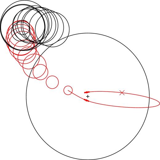
Trajectory and size of a small halo that becomes a subhalo of a larger one and eventually merges with it. Before the halo finder identifies the small halo as a subhalo, its virial radii are shown as small black circles. Their overlapping demonstrates how good the time resolution of our merger trees is. Once the halo finder identifies it as a subhalo (this occurs several time-steps before the subhalo enters the virial radius of the host halo, shown by the large black circle, the sizes of the tidal radii are shown as red circles, the smallest of which denotes the subhalo's last detection in the N-body simulation. The subhalo then becomes a ghost subhalo and its orbit (solid red line) is followed analytically, solving equation (4) in conjunction with equations (5) and (3). The two small red filled circles correspond to the first and the second pericentric passage of the ghost subhalo since the time of last detection. The red cross indicates the position of the subhalo when the dynamical-friction countdown timer comes to zero. The black plus sign denotes the centre of mass of the host system. The thick part of the solid line shows the part of the orbit around the pericentre along which the tides are supposed to act on the stars in the impulsive approximation.
Although our model is not a SAM, we face the same problem of deciding how long a galaxy will survive after it becomes an orphan. Immediately merging the orphan galaxy with the central galaxy of the host system may produce too few satellites and too massive central galaxies. The brute force solution is to increase the number of particles until the results converge above a specified mass. The most commonly followed alternative is to estimate the survival time analytically from the orbital decay time through dynamical friction, tdf (see Knebe et al. 2015; Pujol, Skibba & Gaztañaga 2017, for an overview of the orphan problem in SAMs of galaxy formation).
In its simplest version, this assumption is coupled to that of progressive decay on circular orbits (Somerville & Primack 1999; Hatton et al. 2003; Cattaneo et al. 2006; Cora 2006; Gargiulo et al. 2015). However, this approach neglects the high typical orbital elongations of satellites (Ghigna et al. 1998), which are important for our analysis because the strength of the tides depends on the pericentric radius. A more sophisticated approach is to track the defunct subhalo's most bound particle until a time tdf has elapsed (De Lucia & Blaizot 2007; Benson 2012; Gonzalez-Perez et al. 2014). Here, we follow a third approach, first applied by Lee & Yi (2013), which consists of following the orbits of ghost suhaloes semi-analytically by integrating their equations of motion in presence of two forces: the gravitational attraction of the host halo (computed assuming an NFW profile) and dynamical friction (the physical reason why satellites lose energy, spiral in and eventually fall on to the central galaxy).
When a subhalo ceases to be identified by the halo finder (more precisely, when it is not the main progenitor of its descendant in the merger tree3), we save its mass Ms, position |${\boldsymbol R}$| and velocity |${\boldsymbol V}$| in the host halo's reference frame at the time of last detection. If the system that disappears is a halo, we treat its descendant's main progenitor as if it was its host. These values are the initial conditions from which we start integrating the equations of motions for the ghost subhalo (the red curve in Fig. 1 shows the orbit of a ghost subhalo computed in this manner after the subhalo was no longer resolved4).
We model the ghost subhalo as point particle of mass Ms that moves under the action of two forces: the gravitational attraction of the host and the dynamical-friction drag. However, we shall soon see that the dynamical-friction drag depends on Ms. Therefore, we cannot integrate the equations of motions without computing the evolution of Ms due to tidal stripping at each time-step. The structure of our calculation is thus as follows. In Section 3.1, we describe our method for computing tidal stripping of ghost haloes, which is based on the instantaneous-tide approximation (the tidal radius of the ghost subhalo at a given time is entirely determined by the configuration of the subhalo–host system at that time, although we never allow the tidal radius to grow again after a ghost halo has been stripped). In Section 3.2, we present the equations of motions that we integrate to compute the orbits of ghost subhaloes. Finally, in Section 3.3, we discuss the time at which we should stop their integration because the satellite galaxy associated with the ghost subhalo has merged with the central one.
3.1 Tidal stripping of ghost subhaloes
Equation (3) has a theoretical justification because it is the prediction of tidal theory in the approximation of circular orbits and instantaneous tide (Appendix A). However, according to this theory, α should be the local logarithmic slope of the DM mean-density profile (α < 0 because density decreases with radius). For an NFW profile, −2.6 ≲ α ≲ −2.2 for R = Rvir, but numerical experiments in Appendix A suggest that the appropriate |α| (the one that gives the correct value of Rt) is even higher (α ≲ −3). For R → 0, α → −1 for an NFW profile. However, the presence of a massive central galaxy could imply that α ≪ −1 even at relatively small radii (Fig. A2). Therefore, the value |α| = 1 assumed by the halo finder is therefore likely to overestimate Rt, at least within the circular-orbit approximation. This is not a problem for the orbits of detected subhaloes, which are computed self-consistently by the N-body simulation, but it is a point that we must consider when computing the tidal radii of ghost subhaloes.
In this article, we compute Rt using α = −3 for all ghost subhaloes and we never allow its value to grow again (although equation 3 is instantaneous and thus gives growing values of Rt between the pericentre and the apocentre). The implications of assuming α = −3 will be discussed in Appendix A, after we have explained all the elements that enter our analysis.
3.2 Orbital motion
A ghost subhalo is assumed to move in the gravitational potential |$\Phi ({\boldsymbol r})$| of the halo directly above it in the hierarchy of substructures. 10 per cent of ghosts are sub-subhaloes. For these systems, Φ is the gravitational potential of the subhalo that contains them. In 46 per cent of these cases (which correspond to 4.6 per cent of all ghost systems), the subhalo merges with its host before the ghost sub-subhalo merges with the subhalo. When this happens, the ghost sub-subhalo is promoted to ghost subhalo and continues its orbital motion in the gravitational potential of the host halo.
3.3 Survival time
The problem of computing the survival time tsurv is that of determining after how many pericentric passages we can stop integrating equation (4) because we can consider that the satellite galaxy has merged with the central galaxy of the host halo. Our calculation is based on a modified version of the standard dynamical friction in Binney & Tremaine (2008), which we briefly rederive to clarify its assumption.
On eccentric orbits, ρh varies on a time-scale tdyn ≪ tdf invalidating equation (10) (see Mamon 1996; Chan, Mamon & Gerbal 1997; Cora, Muzzio & Vergne 1997).6 Furthermore, in equation (10), we could take Ms out of the integral because we assumed it to be constant. Real subhaloes are stripped by the tidal field of the host. This reduces the dynamical-friction force and slows down the orbital decay (Mamon 1987; Yi et al. 2013).
Moster, Naab & White (2013) modelled orphan galaxies/ghost subhaloes in a manner similar to ours. They used equation (10) with A = 2.34, this value being based on idealized simulations of orbital decay by Boylan-Kolchin, Ma & Quataert (2008). Given the mean circularity 〈ε〉 ≃ 0.55 found by Jiang et al., the mean value of A in equation (11) is 1.47. Hence, our dynamical-friction times are shorter than those used by Moster et al. by 40 per cent on average.
The dynamical-friction time tdf computed with equations (10) and (11) sets the initial value of the merging countdown time, which begins to tick for detected and ghost subhaloes at the time they first enter the virial radius. When the time tdf elapses, a subhalo can be at any point of its orbit (orbits shrink by dynamical friction but, for highly elongated orbits, the apocentre may still be far away from the centre of the host). Physically, however, the merger of a satellite galaxy with the central one is expected to occur at a pericentric passage. We therefore assume that a ghost subhalo merges with its host at the pericentric passage that is closest in time to when the merging countdown timer rings (marked by a red cross in the example of Fig. 1).
In formulae, let tentry be the time at which the subhalo enters the virial radius for the first time (the large black circle in Fig. 1 shows Rvir at tentry), let tghost be the time at which the subhalo ceases to be detected (the last red empty circle in Fig. 1) and let tmerg be the time of the pericentric passage at which the galaxy merger takes place (the point where the red curve ends). Then, tdf, ghost ≡ tentry + tdf − tghost is the remaining dynamical-friction countdown timer when the subhalo turns into a ghost subhalo. The survival time of the ghost subhalo from the time it becomes a ghost, tsurv ≡ tmerg − tghost, can be both larger or smaller than tdf, ghost depending on whether the nearest pericentric passage occurs before or after the cosmic time tentry + tdf. However, Fig. 2 shows that most ghost subhaloes (74 per cent) lie on a tight correlation tsurv ≃ tdf, ghost. Nearly all the outliers merge at their first pericentric passage. They are subhaloes that ceased being detected short after a pericentric passage and for which the merging countdown timer rang while they were still detected. As we assume that mergers can occur only at pericentric passages, these subhaloes were obliged to make another orbit even though their merging countdown timer had come to zero.
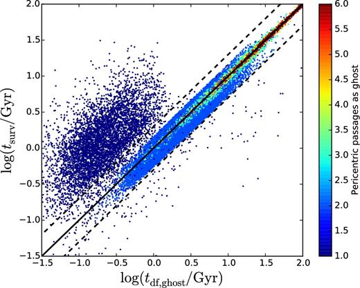
Comparison, for ghost subhaloes, between the expected survival time tdf, ghost based on equations (10) and (11) and the actual survival time tsurv = tmerg − tghost in our model, where mergers can occur only at a pericentric passage. For clarity, we show only 10 per cent of the ghosts of the simulation box. The black solid line represents tsurv = tdf, ghost. The dashed lines correspond to a scatter ±0.3 dex and enclose 74 per cent of the points on the diagram. Points are colour-coded according to the number of pericentric passages between the subhalo's last detection and the merger time in our model. The fractions of ghost subhaloes that merge at the first and the second pericentric passage are 23 per cent and 40 per cent, respectively.
4 THE ENTRY MASSES
This section explains our procedure to assign entry masses to galaxies that enter a group or cluster environment. The entry redshift zentry is the redshift at which the subhalo associated with a satellite galaxy is detected as subhalo of its host for the first time, and differs for each galaxy. Since until zentry all galaxies are central, we can assume that at zentry galaxies still obey the stellar mass–halo mass relation for central galaxies, so that mentry = mc(Mh, zentry), where mc is the stellar mass of the central galaxy for a halo of mass Mh at zentry.
In principle, we could derive mc(Mh, zentry) by solving equation (1), where n* is the SMF of central galaxies at zentry and nh is the HMF (without subhaloes) at zentry. In practice, while it is very easy for a theorist to measure nh in an N-body simulation with or without subhaloes at any redshift, separating central and satellite galaxies in the observations is much more difficult: this requires large spectroscopic surveys and has only been done so far for local data (the Main Galaxy Sample of the SDSS, where nearly all galaxies lie at z < 0.2; Yang et al. 2009, 2012). The red dashed line in Fig. 3 shows the SMHM relation that we obtain when we apply the procedure described in this paragraph using Yang et al.’s (2012) measurement of the local SMF of central galaxies on the seventh data release of the SDSS.
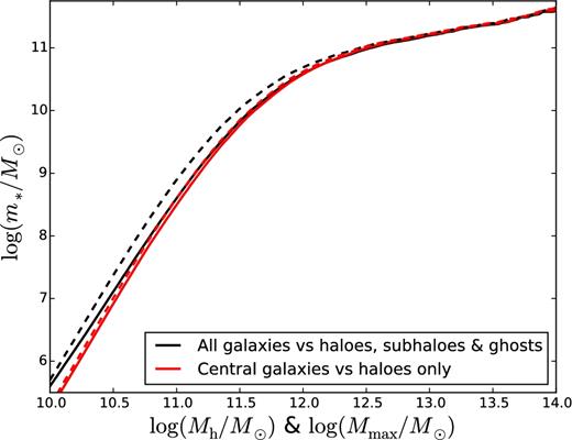
SMHM relation computed by AM (equation 1) using the local (z < 0.2) data of Yang et al. (2012). The AM is performed between the SMF of central galaxies and the HMF without subhaloes (red) or between the total SMF (central and satellite galaxies) to the total mass function of haloes and subhaloes, and ghosts (black). The HMF is computed from the virial mass Mh measured in the N-body simulation at z ≃ 0.1, using the procedure described in Section 2 (dashed lines) or from the maximum virial mass Mmax that a halo/subhalo and its main progenitor ever had over its entire history at z ≳ 0.1 (solid lines).
The problem of this approach is that many of our satellite galaxies have zentry outside the redshift range probed by Yang et al. (2012). Fig. 4 shows the cumulative distribution of zentry for different bins of host–halo (group) mass. The median entry redshift is zentry ≃ 0.1 for Mh > 1013.5 M⊙ but zentry ≃ 0.3 for Mh < 1013.5 M⊙, while less than one satellite in a thousand has zentry > 2.5. At z > 0.2, we only have the total SMF of galaxies, with no splitting between centrals and satellites. To explore the consequences of approximating the SMF of central galaxies with the total SMF, we start by making this approximation in the local Universe, where we know the correct answer mc = mc(Mh) given by the red dashed curve in Fig. 3. If n* is the total SMF and nh is the HMF including subhaloes and ghosts, then equation (1) gives the relation m* = m*(Mh) shown by the black dashed curve in Fig. 3. The difference between the black and the red dashed curves is sufficiently large that approximating the latter with the former would compromise our analysis.
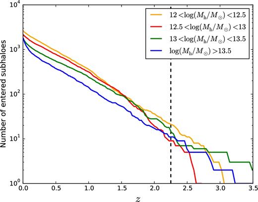
Cumulative distribution of halo entry redshifts for different bins of host-halo mass. The yellow, red, green and blue curves show the mean distribution dN/dz for the entry redshift z = zentry in the bin of host-halo mass 12 < log(Mh/M⊙) ≤ 12.5, 12.5 < log(Mh/M⊙) ≤ 13, 13 < log(Mh/M⊙) ≤ 13.5 and log(Mh/M⊙) > 13.5, respectively. The vertical dashed line at z = 2.5 marks the upper boundary of the redshift range probed by Muzzin et al.’s (2013) data. At z < 0.2, entry masses are computed from the SMF of Yang et al. (2012), who also provided a central/satellite decomposition.
The black dashed curve lies above the red dashed curve because DM haloes are stripped more easily than the compact luminous galaxies at their centres. Subhaloes are stripped more heavily and have higher stellar-to-DM mass ratios m*/Mh than haloes. To demonstrate that tidal stripping of subhaloes is the physical origin for the difference between the black and the red dashed curves, we have recomputed the curves using the maximum mass Mmax that a halo ever had across its history rather than the virial mass Mh at z ≃ 0.1 as an estimator of Mh. In this definition, Mmax cannot decrease. Thus, this procedure removes the effects of mass loss from haloes/subhaloes in our analysis. The relation mc = mc(Mmax) for central galaxies (the red solid line) is very similar to mc = mc(Mh) (the red dashed line) because, for haloes, mass loss is usually negligible. However, the relation m* = m*(Mmax) for all galaxies (the black solid line) is significantly different from m* = m*(Mh) (the black dashed line).
The main conclusion of Fig. 3 is that m*(Mmax) ≃ mc(Mh) for Mmax = Mh (the black solid line and the red dashed line are very close), at least for Mh > 1010.5 M⊙ and m* > 107 M⊙. Thus, we are justified to replace our original assumption mentry = mc(Mh, zentry) with mentry = m*(Mmax, zentry), from which we can compute entry masses at redshifts much larger than z = 0.2.
The observational data that we use for the AM are the SMFs of Yang et al. (2012) at z < 0.2 and of Muzzin et al. (2013) at 0.2 < z < 2.5. To avoid noise, we do the AM using four-parameter double-power-law fits to the observed SMFs rather than the data points themselves. Furthermore, to compute n*(m*, z), we do not use the best-fitting parameters at redshift z. We determine the parameter value at redshift z by fitting a straight line to the evolution with redshift of the best-fitting parameters over six redshift bins covering the range 0 < z < 2.5. The exact fitting formula and the values of the parameters used to fit the SMF are presented in Appendix C. Fig. 5 shows that this model for the galaxy SMF is in good agreement with the data points of both Muzzin et al. (2013) and Yang et al. (2012).
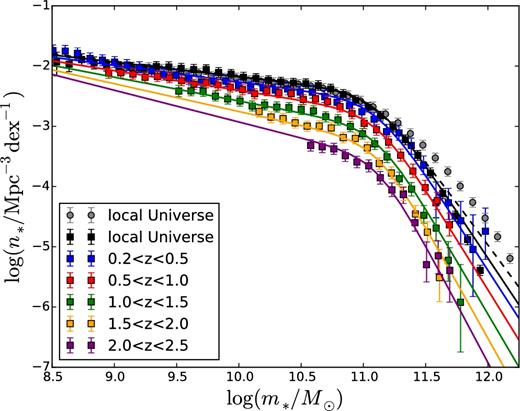
Observed SMFs used to compute the SMHM relation in Figs 3 and 6. The local data (z < 0.2, black squares) are from Yang et al. (2012). The data at 0.2 < z < 2.5 (blue, red, green, yellow and purple squares) are from Muzzin et al. (2013). The SMFs in the six redshift bins were fitted with a double-power-law model (curves), the parameters of which were assumed to vary linearly with redshift. See Appendix C for more details about the fit. The black, blue, red, green, yellow and purple curves show our fits at z = 0.1, 0.35, 0.75, 1.25, 1.75, 2.25, respectively. The grey circles are data from Bernardi et al. (2013) (z < 0.2). They have not been used to fit the evolution of the SMF, but are shown for comparison. The dashed black curve is the fit we would have obtain by fitting Muzzin et al.’s (2013) data only and extrapolating them at z ∼ 0.1. The quality of the fit to the black symbols and the small difference between the solid and dashed black curves proves the overall consistency of Muzzin et al.’s (2013) and Yang et al.’s (2012) data.
To assess the consistency of the two data sets, we have computed the local SMF by extrapolating the data of Muzzin et al. (2013) to z ∼ 0.1, without including the data of Yang et al. (2012) in the fit. The result (the black dashed line in Fig. 5) is intermediate between the SMFs of Yang et al. (2012) and Bernardi et al. (2013), but much closer to the former than to the latter.
Fig. 6 summarizes the results of this section by showing the m*–Mmax relation from AM at three different redshifts (z = 0, 1, 2). The black curve (z = 0) is smooth up to Mmax ≃ 1013.3 M⊙, where the effects of low-number statistics in the N-body simulations begins to be important (there are not many clusters in a volume of 106 Mpc3). We also note that, for a fixed halo mass (e.g. Mmax = 1011.5 M⊙), m* is higher at lower z, most likely because there has been more time to convert gas into stars.
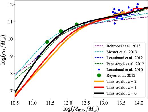
Stellar mass (m*)–halo mass (Mmax) relation used to compute mentry. The relation is computed from AM at all time-steps in the merger tree. For clarity, we show it only at z = 0, 1 and 2 (thick solid black, red and orange curves, respectively). The thin dashed curves show the results of previous studies by Behroozi et al. (2013, purple), Leauthaud et al. (2012, blue), Papastergis et al. (2012, green) and Moster et al. (2013, cyan). The circles are lensing data. Each large green circle is the result of stacking ∼10 000 spiral galaxies (Reyes et al. 2012), while the small blue circles are data points for individual galaxies (Leauthaud et al. 2010).
In Fig. 6, we also compare our SMHM relation at z = 0 with lensing data (Leauthaud et al. 2010; Reyes et al. 2012, circles) and previous AM/HOD models (Behroozi, Wechsler & Conroy 2013; Leauthaud et al. 2012; Papastergis et al. 2012; Moster et al. 2013, curves). The agreement with lensing data is very good considering that lensing observations measure Mh ≤ Mmax. The agreement with previous AM/HOD models is also quite good (particularly in the mass range 1011 M⊙ < Mmax < 1012.5 M⊙), although models differ from one another at the level of 0.1–0.2 dex. The impact that this disagreement may have on our results is discussed in Section 7.1.5. To ease the comparison with future AM work, we provide in Appendix C a fit of our SMHM relation.
5 THE STELLAR MASSES OF SATELLITE GALAXIES TODAY
5.1 Evolution without tidal stripping
We have described the AM method that we used to place a galaxy at the centre of each halo in the volume of our N-body simulations. This procedure determines the stellar masses that satellite galaxies have when they enter a group or cluster environment. We now consider how the masses of these galaxies evolve after their haloes have become subhaloes. Here, we focus on the evolution without tidal stripping of stars, the effects of which will be discussed in detail in the next section.
In standard SAMs, a galaxy is composed of stars and cold gas, and is surrounded by a halo of hot gas. The halo of hot gas accretes mass from the intergalactic medium when the DM halo grows. The hot gas cools and accretes on to the galaxy. The cold gas within the galaxy forms stars. When the galaxy enters a larger system and becomes a satellite, the hot component associated with the galaxy can no longer grow and is depleted by ram-pressure stripping, tidal stripping or cooling on to the galaxy (see McCarthy et al. 2008 for a simple analytical model of how a subhalo is stripped of its hot gas). Only after the halo of hot gas has been stripped down to the size of the galaxy do ram-pressure and tidal stripping begin to remove the cold gas within the galaxy (Bekki 2009). Stars are the last to go because they are impervious to ram pressure and can be stripped only by tides.
The transition from an accretion mode to a starvation mode at zentry is not an assumption of our model. It is a consequence of the fact that subhaloes do not gain mass, they lose it. For most subhaloes, |$\dot{M}_{\rm max}=0$| at z < zentry
In a more extreme scenario, the entire reservoir potentially available for star formation (hot and cold gas) is removed from satellite galaxies upon entry into the host halo. In this ‘shutdown’ scenario, |$\dot{m}_*=0$| for all satellite galaxies at z < zentry. We call this scenario, the shutdown model because it corresponds to a complete shutdown of star formation in satellite galaxies. The shutdown and the starvation models set lower and upper limits, respectively, to the star formation that is possible in group and cluster environments.
The blue and the red curves in Fig. 7 illustrate the qualitative evolution of m* in the starvation and the model, respectively, when we neglect the effects of tides. Tidal stripping transforms the blue curve into the green one and the red curve into the yellow one, but here we focus on models without tidal stripping because we postpone its discussion to Section 5.2.
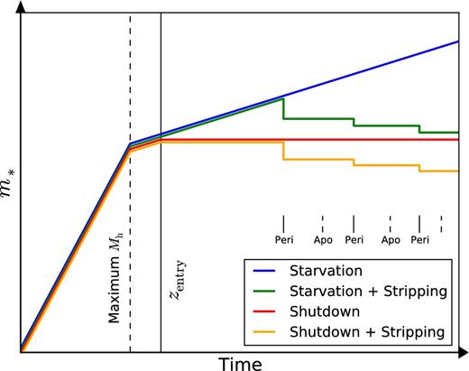
Illustration of our four scenarios for the evolution of stellar mass as a galaxy enters (at time zentry, black vertical bar) and orbits (at times peri and apo for pericentres and apocentres, respectively) in a group or cluster (and thus transitions from a central in a small group before entry to a satellite in a larger group or cluster after entry therein). In all four models, the stellar mass first grows as expected from AM with the current halo maximum mass, once the (sub)halo mass reaches its maximum value (black dashed vertical bar), the stellar mass grows more slowly until zentry is reached. In the shutdown model (red), the stellar mass after entry is maintained at the value at entry. In the starvation model (blue), the stellar mass increases following the AM prescription. Tidal stripping occurs at orbit pericentres (orange and green for shutdown and starvation, respectively). After the first stars have been stripped no more star formation is allowed. Satellite mergers are not considered in this illustration.
In models without stripping, there is no mechanism that can remove stellar mass from galaxies, Hence at each time-step, the stellar mass of a central galaxy is updated to the maximum between the sum of the stellar masses of its progenitors7 and the mass predicted by the m*–Mmax relation at the current z. However, requiring that the mass of a central galaxy be the largest between the sums of the stellar masses of its progenitors and the mass from AM method overestimates the masses of cD galaxies because the masses from AM already includes the effects of mergers. This assumption applies to both the shutdown and the starvation models.
We deal with this problem by introducing a maximum halo mass Mlim, above which we assume that dissipationless mergers are the only opportunity for galaxies to grow. Mlim is a free parameter to be determined by fitting the SMF of galaxies (Section 6.1). In haloes with Mmax > Mlim, m* is the sum of the stellar masses of the progenitors independently of what the AM relation prescribes. The condition that m*(Mmax) can never be lower than the value set by the AM relation is recovered in the limit Mlim → ∞.
5.2 Tidal stripping of stellar mass
We now need to estimate the effects of tidal stripping on the stellar mass of the subhaloes. As a gravitational dynamical process, tidal stripping does not distinguish between a star and DM particle. Therefore, the tidal radius, rt of the stellar distribution should match the tidal radius, Rt of the subhalo, which we computed in Section 3.1 for the DM, especially if we neglect the different dynamical structures of discs and haloes, which is beyond the scope of our analysis, particularly since we do not distinguish between satellites of different morphological types.
However, while a subhalo loses an important fraction of its DM mass before its first pericentric passage (Klimentowski et al. 2009; although we cannot exclude that this may be due to incomplete relaxation of the subhalo), the more concentrated stellar component is stripped almost entirely at pericentric passages (strong variations of the tidal acceleration along elongated orbits lead to a tidal shock at pericentre; Ostriker, Spitzer & Chevalier 1972 and fig. 3 of Klimentowski et al. 2009). Fig. 7 illustrates the qualitative effect of adding tidal stripping on elongated orbits to our shutdown (now orange) and starvation (now green) models. Since most satellite galaxies/subhaloes are on elongated orbits (Ghigna et al. 1998), an impulsive model for tidal stripping of stars is justified. In contrast, the circular-orbit approximation behind equation (3) leads to errors that are too large.
Although the ICL is, by definition, intracluster, i.e. it is not associated with individual galaxies, we can imagine that, in the beginning, stars stripped from galaxies will form tidal tails, which can still be associated with the galaxies from which they originated (e.g. the Magellanic Stream and the Magellanic Clouds). Only later will phase mixing transform these tails into the extended envelopes of central galaxies. We thus begin by storing the stars stripped from individual galaxies in an ICL component that is still associated with the satellites from which it came. When the satellites merge, we transfer the stellar mass in this component to the ICL associated with the outer envelopes of the central galaxy.
Fig. 8 shows the radial dependence of the factor |$\alpha ^2/2/(-2\Phi _{\rm s}/v_{\rm s}^2-1)$|, which sets the maximum efficiency of tidal stripping, for pure DM configuration (black solid curve) and when a disc is embedded in the subhalo (red curve). The figure shows that stripping is less efficient for stars in the central parts of a satellite galaxy. It also shows that εts ≪ 3 everywhere.
![Maximum efficiency of tidal stripping in the impulsive approximation as a function of the distance from the centre of the satellite (rvir is the virial radius of the satellite and α = −3; the real efficiency is the maximum efficiency times [Vc(Rp)/Vp]2). The black curve shows the radial dependence of the maximum efficiency for an NFW potential with c = 8. The red curve shows the effect of embedding in the subhalo a disc of mass 0.04 Mh. These values correspond to the maximum mstars/Mh ratio allowed by AM and to λ = 0.05, respectively. The horizontal dashed black line correspond to a circular orbit in the Jacobi limit (|α| = −3).](https://oup.silverchair-cdn.com/oup/backfile/Content_public/Journal/mnras/471/4/10.1093_mnras_stx1840/1/m_stx1840fig8.jpeg?Expires=1750287932&Signature=ak2cUesxiZNZm1ZqMocBonIwh7oXA0i0gUwC~aQNXliQp8DLFAubQ5efKx~D4gS9soneolX5cAiOKEgAGespH8mGbQtLtMwRdkUvwxudtkcXb-F99bNet3JYVRo6twJD-s8WYkZLqJjw5i3FjZUZHsXv3Ea02SQckSF2Llwcot0MDCgL0SJvniS~4kzB1VATqoTL2dyC~TJRiORZHjvgFGwSTFNbSsXITfOkgoYMRXPP0a5SQlo5tsygcjVj2TR71N3fVy1ldBrKhHC0RNCDxvC~qasI0s5j54K1npHNFTIp7a7TNtRTcdJ3o8D9wK4Y484rwoM5jnFLAtpFKQkuzg__&Key-Pair-Id=APKAIE5G5CRDK6RD3PGA)
Maximum efficiency of tidal stripping in the impulsive approximation as a function of the distance from the centre of the satellite (rvir is the virial radius of the satellite and α = −3; the real efficiency is the maximum efficiency times [Vc(Rp)/Vp]2). The black curve shows the radial dependence of the maximum efficiency for an NFW potential with c = 8. The red curve shows the effect of embedding in the subhalo a disc of mass 0.04 Mh. These values correspond to the maximum mstars/Mh ratio allowed by AM and to λ = 0.05, respectively. The horizontal dashed black line correspond to a circular orbit in the Jacobi limit (|α| = −3).
Besides the coefficient in Fig. 8, the multiplicative factor [Vc(Rp)/Vp]2 < 1 is the only significant difference between the results of the impulsive approximation (equation 18) and the instantaneous approximation (equation 3).
Fig. 9 compares the tidal radii for our impulsive model (equation 21; solid curves), the model of Mamon (dashed curves) and the instantaneous-tide circular-orbit approximation (filled symbols). By definition, the circular tidal theory is only valid for circular orbits, whereas the impulsive theory is not valid for circular orbits. Hence, we expect the tidal radii computed from the circular theory to be more accurate for orbits with Vp = Vc(Rp) and the tidal radii computed from the impulsive theory to be more accurate for orbits with Vp ≫ Vc(Rp). However, most satellites have elongated orbits. The open symbols in Fig. 9 show the mean elongations, measured by Vp ≫ Vc(Rp), for orbits with different pericentric radii Rp/Rvir, according to Ghigna et al. (1998). Smaller pericentric radii correspond to higher orbital elongations. Comparing the ordinates of the open symbols to those of the filled ones shows that the circular theory underestimates the average tidal radius, particularly for satellites with small pericentric radii, and thus overestimates tidal stripping. Fig. 9 also shows that the simple theory of Mamon (2000) provides a good estimate of the tidal radius for satellites with Rp ∼ 0.1Rvir, although it overestimates the effects of tides for satellites on highly elongated orbits.
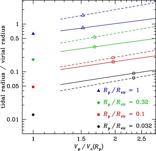
Tidal radii of subhaloes for different orbital elongations (measured by the ratio of pericentre speed to circular velocity at pericentre) and different pericentric radii (colours correspond to different values of Rp/Rvir). This figure compare the estimates from circular tidal theory (equation 3 with α = −3, filled symbols) and from impulsive tidal theory using our full model (equation 18, solid lines) or the approximate formulation of Mamon (2000) (equation 23, dashed lines). The lines stop at Vp/Vc(Rp) = 1.35 because it makes no sense apply the impulsive theory to nearly circular orbits. The open symbols on the solid and dashed lines show the mean Vp/Vc(Rp) for a given Rp/Rvir, computed assuming an average apocentre-to-pericentre ratio of five (Ghigna et al. 1998). As the only purpose of this figure is to compare different approximations, we have assumed that both the host and the subhalo are described by c = 8 NFW models and we have neglected the influence of the baryons on tidal radii.
We therefore compute the tidal radius rt for the stellar component with equation (18), which is more accurate. The implications for our results of using equation (18) rather than equation (3) will be discussed in Section 7.1.3.
The best way to test the validity of our model for tidal stripping is to compare it with idealized (i.e. non-cosmological) numerical simulations, which follow the dynamics of stars more accurately than our analytic calculations while retaining full control of the gravitational potential and the orbital configuration. Kazantzidis, Łokas & Mayer (2013) used idealized simulations to study how tidal stirring can transform a dwarf irregular (a discy dwarf) into a dwarf spheroidal. They assumed a host with the size of the Milky Way and explored three orbital configurations: (Ra, Rp) = (125, 25) kpc, (Ra, Rp) = (125, 50) kpc and (Ra, Rp) = (250, 50) kpc, where Ra and Rp are the apocentric and the pericentric radii, respectively. In the simulations with Rp = 50 kpc, tidal stripping was negligible. For similar orbital configurations, stripping is negligible in our model, too. In the simulation with Rp = 25 kpc, Kazantzidis et al. found the same qualitative behaviour that is shown by the models with stripping in Fig. 7. Quantitatively, the stellar mass of the satellite decreased by 5–10 per cent at each pericentric passage if the stripping potential corresponds to that of an NFW profile, as it does in our model. This figure is broadly consistent with our results, in which a satellite galaxy loses ∼20–25 per cent of its stellar mass over two pericentric passages on average (Section 6).
A more careful examination shows that the agreement is not so straightforward. If we apply our model of tidal stripping to the simulations of Kazantzidis et al. (2013), assuming the same stellar mass and radius as Kazantzidis et al., our model predicts the stellar mass stripped at the first pericentric passage is ∼1 per cent rather than the 5 per cent value found by Kazantzidis et al. in the simulation with (Ra, Rp) = (125, 25) kpc. The stellar mass stripped at each pericentric passage is highly sensitive to both Rp and the radius of the satellite galaxy. The reason why tidal stripping is not negligible in our model despite being much weaker than suggested by Kazantzidis et al. is that the stellar component is less concentrated in our galaxies than in the dwarf of Kazantzidis et al. However, the comparison should keep in mind that Kazantzidis et al. defined m* as the stellar mass within 0.7 kpc, corresponding to 1.7 exponential radii of the disc of the satellite galaxy. Observationally, disc galaxies in the central regions (r < 0.1r200) of clusters tend to have surface-brightness profiles with residuals above an exponential fit at large radii (they have a type III ‘antitruncated’ profile; Pranger et al. 2017). Pranger et al. interpreted this observation as a tidal effect. Instead of truncating discs, tides cause them to be more extended by pulling their outer regions. A lot of the stellar mass that Kazantzidis et al. considered as lost because it moved out of the central 0.7 kpc may still be in the disc at slightly larger radii. Our condition for stripping is much stronger because it requires gravitational unbinding (equation 14). Thus, it is not surprising that we find less stripping in our model. The interesting question is what stellar mass loss Kazantzidis et al. would have found if they had defined m* as the total mass of the stars that are gravitationally bound to the satellite. We have no access to their simulations to answer this question.
6 RESULTS
6.1 Total SMF
In Section 5, we have described two models, the shutdown model and the starvation model, each in a version without and a version with tidal stripping. We now compare these four models with the local galaxy SMFs by Yang et al. (2012) and Bernardi et al. (2013; Fig. 10).
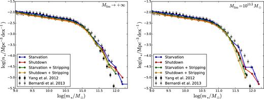
SMFs at z = 0 predicted by our four models (curves, colour-coded as in the legends and in Fig. 7) compared with the observations of Yang et al. (2012; black squares with error bars) and Bernardi et al. (2013; grey circles with error bars). Left: the stellar mass is always the maximum between the stellar mass from AM and the sum of the stellar masses of the progenitors. Right: when the halo mass is Mmax > Mlim = 1013.3 M⊙, the stellar mass is the sum of the masses of the progenitors even when this mass is lower than the value obtained from AM.
At m* ≲ 3 × 10¹¹ M⊙, the four models are indistinguishable from one another and they are all in excellent agreement with the SMF by Yang et al. (2012). However, at m* ≳ 3 × 10¹¹ M⊙, all models tend to be above the SMF of Yang et al. The tendency is stronger for the starvation model without stripping than for the other three models. This finding may seem surprising because the starvation model without stripping applies to all haloes and subhaloes, an AM procedure that should reproduce the SMF of Yang et al., by construction. The discrepancy arises because, if the stellar mass returned by this procedure is smaller than the sums of the stellar masses of the progenitors of a galaxy, it is this sum and not the value returned by the AM procedure that is used to assign a stellar mass to this galaxy. If we assign to all galaxies a mass m* such that the SMF of Yang et al. is reproduced, by construction, and we increase the masses of some of these galaxies (typically, the most massive ones, which have greatest number of progenitors), logically our SMF will contain more massive galaxies than the one of Yang et al. In other words, if all our haloes had a single progenitor, the blue curve in Fig. 10 would fit the square symbols by construction. The discrepancy between the blue curve and square symbols is linked to the merging histories of galaxies. The stellar mass above which the blue curve begins to differ from the SMF of Yang et al. (2012) is the one above which dry (dissipationless) mergers become the dominant growth mechanism and star formation is negligible (Cattaneo et al. 2011; Bernardi et al. 2011a,b).
By enforcing the AM relation, m* = m*(Mmax) even when m* is larger than the sum of the stellar masses of the progenitors, we effectively allow star formation in massive galaxies, which we know to be red from observations (Kauffmann et al. 2003; Baldry et al. 2004). We can deal with this problem by introducing a halo mass limit Mlim, above which m* is simply the sum of the stellar masses of the progenitors, independently of the AM relation (Section 4). This is equivalent to assuming that there is a limit mass, above which dry mergers are the only growth mechanism.
Observations (Kauffmann et al. 2003; Baldry et al. 2004), physical models (Dekel & Birnboim 2006) and SAMs (Bower et al. 2006; Cattaneo et al. 2006; Croton et al. 2006) suggest a limit mass of order 1012 M⊙ (Cattaneo et al. 2006 fitted the colour–magnitude distribution in the SDSS with Mlim ∼ 1012.4 M⊙). We were therefore surprised to discover that the starvation plus stripping model fits the Yang et al. (2012) data for Mlim = 1013.3 M⊙ (Fig. 10b, green curve). Our explanation for this finding is that AM is not a physical model for the baryonic mass that is able to condense to the centre in a halo of given mass: m* is the net result of star formation, dry mergers and stripping. Tidal stripping is responsible for the extended envelopes of giant ellipticals, the masses of which are underestimated by studies based on magnitudes from the SDSS pipeline (Bernardi et al. 2017). Had we calibrated the m*–Mmax relation on the SMF of Bernardi et al. (2013), which includes the light from the outer regions and therefore the debris of tidally disrupted satellites, the green curve in Fig. 10(b) would have shifted to higher masses by an amount comparable to the difference between the SMFs of Yang et al. (2012) and Bernardi et al. (2013). To bring the green curve back on the data points of Yang et al. (2012) would have then required Mlim ≲ 1012.6–1012.7 M⊙ (i.e. the mass limit that shifts the blue curve on the black squares in our calibration), in better agreement with previous studies.
6.2 Conditional SMF
The conditional SMF N(m*|Mh) is defined so that N(m*|Mh) dm* is the average number of galaxies with mass between m* and m* + dm* in a host halo of mass Mh (we have omitted the dependence on z because, in this section, we are only interested in the local Universe). It can be split into the contributions of central and satellite galaxies, in which case the former integrates to unity (there is only one central galaxy per halo).
In this section, we compare the four models in Fig. 10(b) to the conditional SMF measured by Yang et al. (2012). A meaningful comparison requires: (i) that we apply their same definition of host-halo mass and (ii) that we apply their same criterion to decide which galaxies belong to a group or cluster.
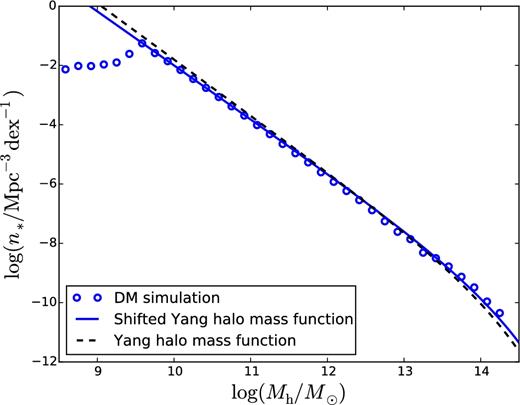
HMF assumed by Yang et al. (2012; black dashed curve) compared to the one that we extract from our N-body simulation (blue circles). The Yang et al. HMF (HMF) is mapped into our extracted HMF with a linear transformation log Mh ↦ alog Mh + b, where a and b are fit to our HMF, and the best-fitting HMF is shown as the blue curve. The blue circles show clearly the resolution of our N-body simulations, which contains 10243 particles in a comoving volume of (100 Mpc)3.
For point (ii), we have re-analysed the density profiles of Yang et al.’s (2012) groups and verified that they are truncated at R180, the radius within which the mean density equals 180 times the mean density of the Universe. R180/Rvir depends on concentration. We have computed R180 for all haloes in the N-body simulations and used this radius to decide which satellite galaxies should be assigned to a host when computing the conditional SMF.
Fig. 12 compares the conditional SMF in our four models with Yang et al.’s (2012) data after taking points (i) and (ii) into account. A number of conclusions can be drawn from this comparison.
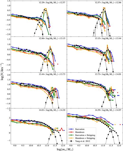
Conditional SMF for our different models (thick solid curves, see legends and Fig. 7) compared to the observations of Yang et al. (2012; black points with error bars). The panels correspond to bins of group mass. Squares and circles show Yang et al.’s decomposition of the data in central and satellite galaxies. The same decomposition has been applied to the models. In models with stripping (green and orange curves), the tidal radius rt has been computed with equation (18). The thin green dashed curves show how the green thick curves vary when we introduce a scatter of 0.2 dex in SMHM relation. They are medians over a hundred realizations. The upper and lower envelopes of the green shaded areas around them correspond to upper and lower quartiles, respectively. In all panels, Mlim = 1013.3 M⊙ (see Section 6.1).
First, the difference between the blue curve and the green one (or the red curve and the orange one) is usually smaller than the difference between the blue curve and the red one. In other words, the effects of stripping are smaller than the uncertainty from our ignorance of the stellar mass Δm* formed after tentry.
Second, all our models predict an excess of massive satellites in low-mass groups (Mh < 1013.44 M⊙), though, at m* < 1010.5–1011 M⊙, data points for satellites tend to lie in the range allowed by our models (between the blue and the orange curves).
Third, the starvation model with tidal stripping (green curves) is the one that, despite this problem, is overall in best agreement with the conditional SMF of Yang et al. (2012) (our N-body simulation contains very few clusters; therefore, the last two panels in Fig. 12 are affected by poor statistics). Fig. 12 was plotted for Mlim = 1013.3 M⊙, but these conclusions are based on the conditional SMF of satellite galaxies, the masses of which are insensitive to the value of Mlim.
Tidal stripping reduces the total stellar mass of satellite galaxies by typically 0.1 dex (0.2 dex at most, green versus blue and orange versus red curves).
The starvation model with tidal stripping (green curve) and the shutdown model without tidal stripping (red curve) provide a comparably good fit to the total stellar mass of satellites in a group.

Therefore, if we were to draw a conclusion based on the total stellar mass of satellites alone, we should concede that there is a degeneracy between the gas mass that accretes on to galaxies and the stellar mass that is stripped from them, and that a model with stellar mass loss intermediate between the predictions of the shutdown and the starvation models (between the red and the blue curves) could fit the observed conditional SMF without the need for any tidal stripping. Nevertheless, tidal stripping is expected to occur on physical grounds. Furthermore, there is observational evidence outside this work that the shutdown of star formation in satellite galaxies is not instantaneous (see the discussion in Section 7.1.2, and references therein). Hence, it is re-assuring that the most astrophysically plausible model is the one that returns a comparatively best fit to the data in Figs 10 and 11.
6.3 ICL
As an independent test of our model, we have compared our predictions for the contribution of cD galaxies (inclusive of the ICL) to the total stellar masses of clusters with the observations of Gonzalez et al. (2013). Fig. 14 shows that, although there are very few clusters in our N-body simulations, our starvation plus tidal stripping model (green circles) matches the observed trend (crosses) for the ratio of BCG+ICL stellar mass over total stellar mass.
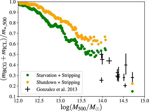
Fractional contribution of cD galaxy inclusive of its ICL to the total stellar mass of a group or a cluster. Only models with tidal stripping display an ICL component. Green and orange circles refer to the starvation model and the shutdown model, respectively. The crosses are the error bars for the observations of Gonzalez et al. (2013). Model predictions have been shown as a function of M500 (the total mass enclosed in sphere of radius R500, within which the average density equals 500 times the critical density of the Universe) to match the definition of cluster mass used by Gonzalez et al. (2013).
More interesting (but more difficult to compare with observations) is the contribution of the ICL to the total stellar mass within a cluster. Fig. 15 shows this contribution when we consider not only the extended envelops of cD galaxies but all stars stripped from galaxies over the entire cluster out to Rvir. It shows that stellar mass fraction in the ICL increases with halo mass.
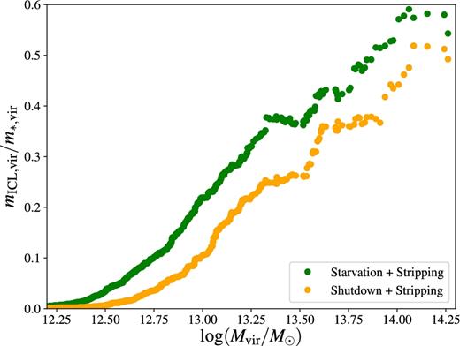
Fractional contribution of the outer envelopes to the total stellar masses within R500. This represent the total diffuse light fraction within Rvir. The model with gas accretion (green) allows for more stripping than the model in which accretion shuts down immediately when a galaxy becomes a satellite (orange).
In Fig. 14, we had shown the BCG+ICL mass fraction within R500 (the radius of a sphere within which the mean density equals 500 times the critical density of the Universe) for consistency with Gonzalez et al. (2013). In our cosmology, the virial radius corresponds to Δc = 102 at z = 0, but we find that the ratio of the ICL mass mICL to the total stellar mass m* is very similar within Rvir and R500 for haloes up to ∼1013.5 M⊙. In clusters, mICL/m* is ∼20 per cent smaller within R500 than it is within Rvir. The implication is that the ICL is more concentrated than the total light of the cluster.9 Fig. 15 shows that, in clusters, the ICL, defined as the total stellar mass stripped from galaxies, whether it still forms a tidal stream around the galaxies themselves or whether it has merged into the extended envelope of a cD galaxy, may amount to nearly half of the total stellar mass with Rvir.
In an article that appeared when ours was about to be submitted, Bernardi et al. (2017) argued against the interpretation that difference between the SMFs of Baldry et al. (2012) and Bernardi et al. (2013) is due to the ICL. Their claim is that the difference is entirely due to the different way the photometry is done. The magnitude provided by the SDSS are based on fitting an exponential and a de Vaucouleurs surface-brightness profile separately and retaining the value for the profile that fits better. The python image-morphology software pymorph fits the surface-brightness profiles of galaxies much more accurately because it allows for the presence of both an exponential and a Sérsic component. Bernardi et al. (2017) correctly argued that the difference is more than semantic because there is no doubt that a model with five free parameters can fit the surface-brightness profiles of galaxies more accurately than a model with two and thus return more accurate photometry.
As a Sérsic-exponential profile provides an excellent fit to the surface-brightness profiles of luminous red galaxies out to eight effective radii (about 100 kpc), Bernardi et al. (2017) concluded that the difference between pymorph and SDSS magnitudes cannot be due to the ICL. This conclusion is based on the fact that they define the ICL as any residual luminosity above the Sérsic-exponential fit. This definition is entirely reasonable from an observers standpoint. However, the Sérsic-exponential profile is nothing more than a useful fitting formula. Another functional form with more free parameters may fit the surface-brightness profile far beyond eight effective radii, eliminating the need for the ICL altogether. We do not question the claim by Bernardi et al. (2017) that pymorph returns objectively more accurate magnitudes than the SDSS pipeline. We enquire about the physical reason why giant ellipticals have extended light profiles, be they or not above a Sérsic-exponential fit. Following Gallagher & Ostriker (1972), we pursue the hypothesis that the extended envelopes of giant ellipticals are the debris of tidally disrupted galaxies, and define the ICL as the light from stars that have been tidally stripped from galaxies. This definition is of no assistance to an observer who wishes to measure the ICL. However, it is significant that when we compute the ICL mass according to our definition, we recover a lot of the difference between the SMFs of Baldry et al. (2012) and (Bernardi et al. 2013, see Fig. 10, the gap between the blue and the green curves).
Bernardi et al. (2017) have also argued that the ICL should be centred on the centres of the clusters and should thus affect the magnitudes of central galaxies more than it affects those of satellites, while their work shows that, for a same luminosity, the difference between pymorph and SDSS magnitudes is about the same for both central and satellite galaxies. However, this is not a problem if one adopts our definition of the ICL because tidal stripping is expected to affect satellite galaxies, too. In fact, satellite galaxies will first develop long tidal tails and then these tails will coalesce into the extended envelopes of the central systems. This is how minor mergers have plausibly contributed to the considerable size evolution of elliptical galaxies from z = 2 to the present (e.g. Naab & Ostriker 2009; van Dokkum et al. 2010; Tal & van Dokkum 2011; Cooper et al. 2012; Shankar et al. 2013).
7 DISCUSSION
In this section, we discuss the uncertainties that affect our results. They come from (i) the resolution of the N-body simulation and the model for orphan galaxies that we have introduced to overcome the effects of limited resolution; (ii) uncertainties regarding the amount of star formation a satellite galaxy experiences post accretion on to the host halo; (iii) uncertainties regarding the amount of stellar mass loss experienced by satellite galaxies as a consequence of tidal stripping and heating; (iv) scatter in the SMHM relation; and (v) the AM method itself. We also discuss the excess of massive satellites in groups with Mh < 1013.44 M⊙ predicted by all our models.
7.1 Model uncertainties
7.1.1 N-body resolution and orphan galaxies
In Section 3.2, we have treated ghost subhaloes as systems with well-defined orbits in a static spherical potential. Cosmological haloes contain substructures that contribute to their gravitational masses and perturb the orbital motions of subhaloes. Our work does not consider the contribution of substructures to the gravitational potential of their host because our calculations are based on exclusive masses (our halo masses do not include the masses of substructures). We made this choice because the NFW model fits the density profiles of DM haloes more accurately when substructures are removed. If the mass distribution of substructures followed the NFW profile of the host halo, their merging time-scales would be shorter by typically 10 per cent. In reality, it is entirely possible that the interaction with other substructures may scatter a subhalo on an orbit with a longer merging time-scale. However, Hayashi, Navarro & Springel (2007) have shown that the isopotential surfaces inside a halo are much smoother than the density distribution and relatively insensitive to the presence of substructure.
The assumption that haloes are spherical is another simplification. Real haloes are triaxial. At z = 0, the typical minor-to-major axis ratio of the virial ellipsoid ranges from 0.75 at Mh ∼ 1011 M⊙ to 0.5 at Mh ∼ 3 × 10¹⁴ M⊙ (Despali et al. 2017). Triaxiality increases at small radii but dissipation makes DM haloes substantially rounder at small radii than suggested by dissipationless simulations (Springel, White & Hernquist 2004). Furthermore, as expected from Poisson's equation, the gravitational potential tends to be much more spherical than the mass distribution. Indeed, Hayashi et al. (2007) find that a flattening (minor-to-major axis ratio) of ∼0.4 in the mass distribution corresponds to a flattening of only ∼0.75 for the isopotential contours the minor-to-major axis ratios of the isopotential contours are ≈0.75, hence much greater than the corresponding ratios for the density contours (≈0.4).
In this work, the approximation of a static spherical potential applies to ghost subhaloes only. At a given stellar mass, the fraction of satellite galaxies with unresolved (ghost) subhaloes depends on the resolution of the N-body simulation. If all subhaloes of satellite galaxies with m* > 109 M⊙ were resolved, our results would be independent of this approximation. Hence, while it is difficult to estimate, a priori, the errors introduced by treating ghost subhaloes as systems with well-defined orbits in a static spherical potential, it is easy to do it, a posteriori, by performing resolution studies.
To test the sensitivity of our results to N-body resolution and to our modelling of orphan galaxies, we have repeated our entire analysis on a simulation with the same cosmology, the same volume, the same initial conditions, but only 5123 particles instead of 10243, and we allow ourselves to immediately merge orphan galaxies with the central galaxy of their host halo (i.e. to use the original merger tree without the addition of ghosts and orphan galaxies). We focus the comparison on our best-fitting model (starvation plus stripping) and on the mass range 1013.44 M⊙ < Mh < 1013.73 M⊙, but the results for this case also apply to the other models and mass bins.
Fig. 16 compares the conditional SMF for this model and mass range varying the resolution of the simulation and the treatment of orphans. With 5123 particles, the conditional SMFs with (solid purple curve) and without (dashed purple curve) orphans differ at m* ≲ 1010 M⊙. However, with 10243 particles, the resolution is so good that delaying the mergers of orphans with central galaxies (solid green curve) or not (dashed green curve) makes little difference above m* = 108.5 M⊙. The treatment of orphans is a small correction and therefore a negligible source of uncertainty in relation to our conclusions.
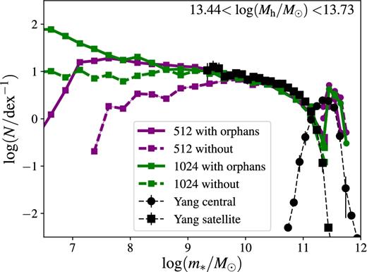
Sensitivity of the conditional SMF predicted by the starvation+stripping model to the resolution of the N-body simulation, degraded from 10243 (green) to 5123 particles (purple lines), and to the merger time of orphan galaxies with the central galaxy: immediately (dashed lines) or only at the first pericentre following the expected time of orbital decay by dynamical friction (solid lines). The figure shows the case for haloes with 13.44 < log (Mh/M⊙) < 13.73. In the mass range probed by the observations (Yang et al. 2012; black symbols with error bars), the model with orphan galaxies has converged because the simulations with 5123 and 10243 particles give very similar conditional SMFs.
Above m* ∼ 1010 M⊙, the conditional SMFs for the 5123 simulation without orphans (dashed purple curve) and the 10243 simulation without orphans (dashed green curve) are very similar, suggesting that numerical convergence has been reached. Most interesting, however, is the agreement of the 5123 and 10243 simulations when orphans are included, as we see convergence (solid green and purple lines) in the conditional SMF down to 107.7 M⊙. This proves that the inclusion of orphans aids in achieving convergence to correct solution (also see Guo et al. 2011). At m* ≳ 3 × 10⁸ M⊙, the 5123 simulation with orphans is at least as good as the 10243 simulation without orphans.
7.1.2 Gas accretion on to satellites
Estimating how much gas accretes on to satellite galaxies after entering a group or cluster environment is less straightforward than testing for resolution effects, but the simple assumption that star formation shuts down immediately cannot be correct. Weinmann et al. (2006) used a version of the Munich SAM in which there was no accretion on to satellite galaxies (Croton et al. 2006). They found that the fraction of faint satellites with red colours was overestimated by a factor of ∼2–3. All SAMs published in those years shared the same problem (e.g. Fontanot et al. 2009). Indeed, Cattaneo et al. (2007) ran the GalICS SAM on merger trees from a cosmological hydrodynamic simulation. GalICS assumed no gas accretion on satellites and predicted a much higher fraction of quenched galaxies than the hydrodynamic simulation.
A delayed quenching scenario can be parametrized by two time-scales: the time tdelay during which a galaxy keeps forming stars after entering a group or a cluster and the tquench, over which the star formation rate rapidly decays after tdelay has elapsed. Several authors have investigated these time-scales. Mahajan, Mamon & Raychaudhury (2011) split galaxies between infalling, backsplash and virialized, and combined the fraction of star-forming galaxies observed in the SDSS with cosmological N-body simulations to quantify projection effects. Their analysis suggests that quenching is delayed until galaxies reach the virial radius on their way out of the cluster after the first pericentric passage. As shown in Fig. B1 in Appendix B, galaxies that are at the virial radius today, on their way out after their first pericentric passage, and have typical first apocentres close to the turnaround radius at that time (3–4 virial radii at that time), entered the group/cluster environment ∼3 Gyr ago (Fig. B1 in Appendix B), and passed through the pericentre ∼1.6 Gyr ago. Therefore, according to the modelling of Mahajan et al., star formation is quenched ∼3 Gyr after cluster entry and ∼1.6 Gyr after the first pericentric passage. Wetzel et al. (2013) used an N-body simulation to measure the characteristic time, since tentry of a galaxy at a given R/Rvir, and constrained tdelay and tquench by measuring the fraction of red galaxies in SDSS groups/clusters as a function of the distance from the centre. A slow progressive fading of star formation since tentry would blur the bimodal distribution of galaxy colour. In contrast, the observations are consistent with a long delay (tdelay = 2–4 Gyr) followed by rapid quenching (tquench = 0.2–0.8 Gyr). Haines et al. (2015) performed a similar study to match the observed distribution of the fraction of star-forming galaxies with the predictions of times since entry as a function of position in projected phase space from cosmological N-body simulations. They conclude that star formation declines exponentially after entering the virial radius on a time-scale of 1.7 Gyr. A similar analysis by Oman & Hudson (2016) suggests that star formation in cluster satellite galaxies is rapidly quenched within ∼1–2 Gyr from the first pericentric passage. Another recent similar study based on both SDSS and higher redshift data leads to delay times of 2–5 Gyr (Fossati et al. 2017).
Further evidence in support of delayed quenching comes from chemical abundances. When a galaxy ceases to accrete pristine gas but keeps forming stars, its metal content relative to hydrogen increases. From the metal abundances of red galaxies with m* ≲ 1010.5 M⊙, Peng et al. (2015) inferred that they must have behaved as closed boxes for ∼ 4 Gyr before they eventually run out of gas. The higher metallicities of satellite galaxies were interpreted as evidence that this is due to starvation by the environment. While the complete starvation of gas accretion in Peng et al.’s picture seems to conflict with SAMs.10 There is consensus that star formation cannot have been quenched instantaneously at tentry.
In conclusion, while it is not straightforward to determine what fraction of the gas associated with a subhalo will accrete on to the satellite galaxy it contains and what fraction will be stripped (mainly by ram pressure, which is more important than tidal stripping for gas11), and while the precise value will also depend on the feedback one assumes (Tomozeiu, Mayer & Quinn 2016), there appears to be observational consensus that star formation is quenched 1–2 Gyr after the first pericentric passage. Therefore, the starvation model, which prevents further accretion from the environment but allows star formation to continue until the first pericentric passage, seems a much more plausible assumption than to assume a complete shutdown of star formation at the entry time.
7.1.3 Tidal stripping
Tidal stripping is an inevitable dynamical process, but its analytic modelling is not straightforward and requires simplifying assumptions. The most common assumption is instantaneous tides applied to satellites are on circular orbits. However, for a fixed pericentric radius, this assumption gives an upper limit rather than a realistic estimate for the stellar mass that is tidally stripped from galaxies because most orbits are highly elongated. The circular-orbit approximation underpredicts the conditional SMF even when it is applied to the starvation model, which corresponds to the maximum possible star formation in satellite galaxies (green curve in Fig. 17) because it results in stellar mass loss of satellite galaxies that can be as large as 0.5 dex. On the contrary, the difference between the starvation model without stripping (blue curve) and the observations (horizontal black line) in Fig. 13 shows that the stellar mass that can plausibly be stripped from galaxies is ≲0.15–0.2 dex (≲0.1–0.15 dex if we allow for ≳10 per cent stellar mass loss through stellar evolution between zentry and z = 0). This upper limit is obtained by comparing a model without stripping to the observations. It is therefore totally independent of any physical model of tidal stripping.
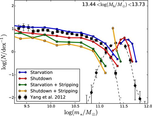
Conditional SMF for our different models (curves) compared to the observations of Yang et al. (2012; black data points with error bars). This figure is identical to the 1013.44 M⊙ < Mh < 1013.73 M⊙ panel of Fig. 12 except for the calculation of tidal stripping (the green and orange curves). Here, tidal stripping is computed in the circular-orbit instantaneous-tide approximation, using equation (3) with α = −3.
Re-assuringly, the more sophisticated model in Section 5.2 predicts tidal stripping by ∼0.1 dex (∼25 per cent) on average, in agreement with the upper limit above. This value (based on the green curve in Fig. 13) has been computed assuming the maximum tidal acceleration but also assuming that the tidal acceleration acts only for a very short time around the pericentric passage (corresponding to the part of the orbit shown as a thick solid red line in Fig. 1). Using the average acceleration for a test particle (equal to half the maximum acceleration; Appendix A) while retaining the second assumption will most likely underestimate the tides. However, this results in an average tidal stripping of 0.07–0.08 dex on average, so the quantitative difference is small.
The assumption of circular orbits is as incorrect for the DM as it is for the stars, but we kept using it to compute the DM lost by ghost subhaloes because DM is stripped all the way down to the centre, not just at pericentre (Klimentowski et al. 2009), so the impulsive approximation is not necessarily much more accurate. The question is the extent to which its inaccuracy affects our conclusions. Tidal radii have no consequences on the survival times of ghost subhaloes, which are by Jiang et al.’s (2008) formula. Their only effect on the tidal stripping of stars is through the value of Rp. If a ghost subhalo is stripped too heavily (the most likely outcome of our approximation), it will suffer less dynamical friction. Less dynamical friction implies less orbital decay. The pericentric radius will be overestimated and the tidal stripping of stars will be less efficient than for the correct value of Rp. Therefore, we can be confident that 0.07–0.08 dex is a plausible lower limit for the stellar mass lost by galaxies owing to dynamical friction.
In practice, ghost subhaloes (and thus this calculation) were introduced as a way to beat the resolution limit of our N-body simulation. A posteriori, our resolution is so good that conditional SMFs are very similar with or without them (Fig. 16). Thus, any error in our calculation of the pericentric radii of ghost subhaloes is bound to have a limited impact on the conclusions of this article.
7.1.4 Scatter in the SMHM relation
Our AM procedure (Section 1.2) assumes that the m*–Mmax relation does not contain any scatter. In this section, we discuss how scatter can affect our conclusions.
Observationally, to determine the scatter in stellar mass at constant halo mass, one needs a method to measure Mh. Yang et al. (2009) estimated the masses of groups from their luminosities (Section 6.2) and found a scatter in log m* of |$\sigma _{{\rm log}\,\,m_*}\simeq 0.17\,\,$|dex in m* at constant Mh. More et al. (2009) found a similar result (|$\sigma _{{\rm log}\,\,m_*}\simeq 0.16\,\,$|dex) using halo masses from satellite kinematics. Leauthaud et al. (2012) performed a more sophisticated analysis by fitting simultaneously the galaxy SMF, clustering data (correlation functions) and halo masses from galaxy–galaxy lensing. They found an intrinsic scatter of about 0.2 dex after subtracting errors from photometry, photometric redshifts and spectral energy distribution fitting. Behroozi et al. (2013) used AM to infer a scatter of 0.22 ± 0.02 dex. Coupon et al. (2015) repeated the same analysis with more recent data and confirmed their results.
Implementing scatter in our models requires a more sophisticated approach than simply applying random errors to the stellar masses determined from the AM relation. If we simply perturbed the AM relation, our models would no longer reproduce the galaxy SMF because of the Eddington bias. We overcome this problem by splitting the galaxy population into pairs. One galaxy has logarithmic stellar mass log m*. The other has logarithmic stellar mass log m* + log Δm*, where log Δm* is a random number from a Gaussian distribution with standard deviation |$\sigma _{{\rm log}\,\,m_*}$| and zero mean. Scatter is implemented by swapping the haloes of the two galaxies. This swapping introduces the requires scatter in the SMHM relation without changing the actual SMF of the galaxies.
This procedure means that the conditional SMFs computed by our models are now dependent on the random way in which galaxy population has been splitted into pairs but we can obtain robust results by averaging over many different realizations. The thin green dashed curves in Fig. 12 show the median conditional SMF for the starvation plus stripping model over a hundred realizations with |$\sigma _{{\rm log}\,\,m_*}=0.2$|, while the green shaded areas show upper and lower quartiles for the same hundred realizations. The absence of systematic differences between the thin and the thick green curves (the model without scatter) proves that scatter adds noise but will not bias our conclusion. Thin lines and shaded areas have been shown for the starvation plus stripping model only not to overcrowd the figure.
7.1.5 Uncertainties in the SMHM relation
Fig. 6 shows that the SMHM relations derived with different AM/HOD models differ at the level of 0.1–0.2 dex in stellar mass. One could interpret these differences as a measure of the intrinsic uncertainty of the SMHM relation from AM. To understand the implications that such an uncertainty may have for our results, we begin by discussing the origin of these differences.
The first source of difference is the SMF used to constrain the SMHM relation. The SMHM relation of Moster et al. (2013) differs from those of other authors at low masses because they used the SMF of Li & White (2009), which contains a higher a number density of galaxies with 109 M⊙ < m* < 1010.2 M⊙ than the SMFs of Baldry, Glazebrook & Driver (2008), Baldry et al. (2012), Leauthaud et al. (2012), Yang et al. (2012), Papastergis et al. (2012) and Moustakas et al. (2013).
Secondly, the HMFs assumed by different authors can come either from N-body simulations or from the Sheth & Tormen (2002) formula, which is calibrated on N-body simulations. Even if the cosmologies assumed by different authors were completely identical, there would still be an uncertainty of about 10 per cent in the HMF from the halo finder (Knebe et al. 2013).
Finally, one can use the AM method, as we have done, or one can assumed a parametric SMHM relation and constrain its parameters so that it fits the SMF. The results obtained with the two methods will be very similar but not necessarily identical. One can also consider or not consider the presence of scatter (Section 7.1.4). Models with scatter find lower stellar masses for a given halo mass at high masses to compensate for the Eddington bias.
We argue that these systematic uncertainties are not important for our conclusions because our analysis focuses on the differences in stellar mass between field and satellite galaxies. We apply the same N-body simulation, the same halo finder and the same AM procedure to both. Therefore, these uncertainties cancel out in the relative comparison, as would any systematic error in the photometry or the initial mass function.
The only real question is whether our SMF n*(m*, z), which is constructed from data at different redshifts (Yang et al. 2012 at z < 0.2, Muzzin et al. 2013 at 0.2 < z < 2.5), is fully consistent with the conditional SMF of Yang et al. (2012), to which we compare our results. Fig. 5 shows that, for 109 M⊙ < m* < 1011.5 M⊙ the local SMF assumed for this work (black solid curve) is fully consistent with both the SMF of Yang et al. (2012; black symbols with error bars) and the SMF of Muzzin et al. (2013) extrapolated to z = 0.1 (black dashed curve).
7.2 The massive satellite excess in low-mass groups
The most noticeable discrepancy between our models and the observations of Yang et al. (2012) is the excess of massive satellites with m* ≳ 1011 M⊙ in low-mass groups (Fig. 12). This excess cannot be due to star formation after zentry or to underestimated stripping because, at Mh ≲ 1013 M⊙ it is present even in the shutdown model when tidal stripping is computed with the instantaneous-tide circular-orbit approximation (which largely overestimates the magnitude of the phenomenon; Section 7.1.1).
There are two possible explanations for this discrepancy. First, Yang et al. (2012) may have classified as central systems that, in the N-body simulation, our halo finder classifies as satellites, see Skibba et al. (2011) and Lange et al. (2017) for a discussion of this phenomena. Bernardi et al. (2017) have analysed SDSS groups with a group finder called redMaPPer, which differ from the one used by Yang et al. (2012). They have remarked that: ‘Many of the objects which Yang et al. classify as being centrals in groups less massive than 1014 M⊙ are called satellites by redMaPPer’. Second, a satellite with m* comparable to the central galaxy in a small group of often 2–3 objects is very different system from a satellite in a cluster, whose total mass is much larger than that of any satellite. The Jiang et al. (2008) formula (combined with our prescription, which requires one galaxy out of four to complete an additional orbit after a time tdf has elapsed since entry) may fail when applied to nearly equal-mass binary systems. If their merging time is systematically overestimated, this could explain the excess of massive satellites in low-mass groups.
8 CONCLUSIONS
The original goal of this work was to estimate the stellar mass lost by galaxies in groups and clustering due to tidal stripping by comparing the distribution of entry masses to observations of the conditional SMF. As our work progressed, we realized that this original approach was too simplistic because the distribution of entry masses (shown by the red curves in Fig. 12, except for satellites that have merged) is below the data points for most values of m*. If we look at the mass variation from zentry to z = 0, then galaxies have gained stellar mass, not lost it.
The simplest refinement of this analysis is to assume that Δmstrip = mentry + Δm* − m*, where mentry is the stellar mass at zentry, Δm* is the mass of the stars formed between zentry and z = 0 and m* is the stellar mass at z = 0. The problem is that Δm* is considerably uncertain. We can obtain an upper limit for Δmstrip by assuming that, in satellite galaxies, stellar mass grows with halo mass following the same relation that holds for central galaxies. This assumption maximizes Δm*. If we follow this approach, we find that the stellar mass loss from satellite galaxies is ≲0.15–0.2 dex. However, this would imply that central and satellite galaxies have similar SFRs. This is inconsistent with observations, which indicate that satellite galaxies have, on average, lower SFRs than centrals of the same stellar mass (i.e. Weinmann et al. 2006; Wetzel et al. 2013, and references therein). Hence, this model clearly has to be regarded an extreme upper limit for Δm*.
The upper limit for Δmstrip includes both the stellar mass lost due to tidal stripping and the decrease in stellar mass that results from stellar evolution. A typical satellite galaxy is accreted into its host halo at a median redshift of zentry ∼ 0.5, which corresponds to a lookback time of ∼5 Gyr. Assuming passive evolution, a typical quiescent galaxy will lose between 10 and 20 per cent of its mass over a period of ∼5 Gyr (e.g. Fioc & Rocca-Volmerange 1997). Accounting for this passive evolution, gives a more stringent upper limit Δmstrip ≲ 0.1–0.15 dex.
This is an upper limit because of the uncertainty on Δm*. Since mentry − m* < 0 and |$m_{\rm entry}+\Delta m_*^{\rm max}-m_*>0$|, it is possible to find a plausible value of Δm* for which Δmstrip = mentry + Δm* − m* = 0, that is, the analysis above cannot rule out a model without stripping.
We have compared this indirect result with direct analytic estimates of the stellar masses that galaxies lose due to tidal stripping. The simplest estimates based on instantaneous tides and circular orbits are highly inaccurate because most satellites are on highly elongated orbits. These estimates predict much more stripping that is allowed by the upper limit derived in this article. More sophisticated estimates assume impulsive stripping on elongated orbits (satellite galaxies lose stars at each pericentric passage). In this article, we have improved previous analytic models of impulsive tides (Spitzer 1958; Gonzalez-Casado et al. 1994; Mamon 2000) and have used our results (equation 18) to predict stripping by 0.07–0.1 dex on average, which is consistent with our upper limit ≲0.1–0.15 dex.
We consider 0.07 dex (17 per cent) to be a reasonable lower limit for the stellar mass lost by galaxies owing to tidal stripping because: (i) its calculation is based on the average rather than the maximum tidal acceleration; (ii) we assumed that the tides acts only for a very short time interval around the pericentre and (iii) pericentric radii that may be overestimated (in case of ghost subhaloes) but not underestimated (tides are stronger for closer pericentric passages).
Our best estimate for the stellar mass lost owing to tidal stripping, ∼0.07–0.1 dex (∼17–25 per cent), is consistent with a picture in which Δm* is close to |$\Delta m_*^{\rm max}$|, i.e. one in which satellite galaxies are quenched several Gyr after entering a group or cluster environment and, in any case, after the first pericentric passage (Mahajan et al. 2011; Wetzel et al. 2013; Haines et al. 2015; Peng et al. 2015; Oman & Hudson 2016; Fossati et al. 2017).
Our model predicts that the fraction of stars that contribute the ICL increase with the mass of the host system. In clusters, stars tidally stripped from galaxies are predicted to contribute to half of the total light within R500.
Acknowledgements
We thank Julien Devriendt for taking care of running the DM simulations used for this work and for computing and providing us the associated merger trees. We also thank the anonymous referee and Marina Trevisan for useful comments. Frank van den Bosch is supported by the Klaus Tschira Foundation and by the US National Science Foundation through grant AST 1516962.
Throughout this article, we use lower case letters for stellar masses and radii within subhaloes, and upper case letters for dark matter (DM) masses and subhalo radial coordinates within haloes.
The formulae of Bryan & Norman (1998) are a fit to the predictions of the spherical top-hat collapse model, but we have assumed that small deviations from sphericity do not change the virial density of DM haloes.
The merger tree is constructed by linking haloes that the halo finder has identified in output files at different time-steps. A halo can have more than one progenitor but at most one descendent. If the halo fragments, its descendent is the fragment that has inherited more than half of its particle. If none of the fragments contain more than half of the particles that the halo finder had assigned to the halo at the previous time-step, the halo is considered to have disappeared. The halo or subhalo is also considered to have disappeared if tidal stripping has been so strong that it has lost more than half of its particles from one time-step to the next because the algorithm that constructs the tree is not able to recognize that the stripped halo is the descendent of its progenitor.
The rapid decrease in size when passing from the black circles to the red circles in Fig. 1 is an artefact of the halo finder.
Duarte & Mamon (2015) solved the Jeans equation of local dynamical equilibrium for a velocity anisotropy |$\beta =1-2\sigma _{\rm r}^2/\sigma _{\rm t}^2$| with the radial dependence β = (1/2)[1 − R/(R + R0)], which Mamon & Łokas (2005) found to match well the velocity anisotropies measured in cosmological simulations (R0 is the scale radius of the NFW profile).
Even on circular orbits, the time-scale for orbital decay can be up to four smaller than predicted by the Chandrasekhar formula, because of resonances between the halo and subhalo (Prugniel & Combes 1992).
By progenitors, we mean the galaxy main progenitor and all the satellites that have merged with it, since the last time-step.
The satellite population is dominated by disc morphologies: spirals, S0s (the spiral arms are no longer visible because all gas has been consumed or removed) and dSphs (discs that puffed up because of either stellar feedback or tidal interactions).
Stripped stars are stored first in an ICL component associated with it parent satellite, when the satellites merge, we transfer the stellar mass in this component to the ICL associated with the central galaxy. Therefore, we define mICL within Rvir (respectively R500) as the sum of the mass of the ICL component from galaxies within Rvir.
The difference is largely due to the assumed star formation efficiencies. SAMs usually assume shorter star formation time-scales than those of Peng et al. (2015), at least at low stellar mass. Hence, they need sustained accretion to keep star formation going for several Gyr.
In field galaxies, Hi discs are more extended than stellar discs. In satellite galaxies, it is often the contrary because ram pressure has stripped their outer parts. Where tidal stripping the dominant phenomenon, the Hi disc would be truncated at the same radius as the stellar disc because tides do not differentiate between gas and stars.
Throughout this appendix, lowercase letters refer to distances from S and uppercase letters to distances from H.
REFERENCES
APPENDIX A: THEORY OF TIDES IN THE CIRCULAR-ORBIT APPROXIMATION
In this appendix, we compute the tidal acceleration |${\boldsymbol a}_{\rm t}$| that a host system exerts on a test particle of a satellite. We also compute the tidal radius rt of the satellite in the approximations that: (i) the satellite is on a circular orbit, so that the gravitational potential is static in a corotating frame, and (ii) the test particle is instantaneously stripped as soon as |${\boldsymbol a}_{\rm t}$| exceeds the gravitational acceleration that keeps the particle bound to the satellite. The latter is an approximation because a net outward acceleration is a necessary but not sufficient condition for tidal stripping. For it to be sufficient, the speed |$\int {\boldsymbol a}_{\rm t}{\rm \,\,d}t$| imparted by the acceleration to the particle must be large enough to unbind it. In Section 5.2, we build on these results and generalize them to non-circular orbits and non-instantaneous tides.
Fig. A1 shows the equipotential contours for Φeff in a particular case used for illustrative purposes. In this particular case, Ms/Mh = 0.1, |$\overline{\rm HS}=R_{\rm vir}$|, and both the host and the satellite are described by an NFW profile with concentration c = 8 (Rvir is the host virial radius). The equipotential contours show a saddle point L1 on the segment HS, which is the First Lagrangian Point L1, which separates the Roche lobes of the host and the satellite. The particle P is tidally stripped if its orbit spills outside the Roche lobe of the satellite. In the next five paragraphs, we shall calculate |$r_{\rm t}\sim \bar{\rm SL_1}$| in the limit that: (v) Ms ≪ Mh, so that O → H, and (vi) |$\overline{\rm SP}\ll \overline{\rm HS}$|, so that we can expand |${\boldsymbol a}_{\rm t}$| in powers of r/R (Jacobi limit). However, it is important to understand that, even if |$\bar{\rm SL_1}$| could be computed exactly, it would still provide an approximate estimate for rt because a circle of radius |$\bar{\rm SL_1}$| and centre S lies outside the Roche lobe of the satellite. The implication is that the real tidal radius is |$r_{\rm t}<\bar{\rm SL_1}$|.
Equipotential curves for the effective potential Φeff (equation A4) of a two-body system composed of a host halo and a subhalo, centred on H and S, respectively (contours). H and S are on circular orbits around the centre of mass O of the two-body system. The First Lagrangian Point L1 separates the Roche lobes of the host and the satellite. P is a test particle within the subhalo. The figure is for a satellite-to-host mass ratio of Ms/Mh = 0.1. It assumes that both the host halo and the subhalo are described by an NFW profile with c = 8 and that the subhalo lies at the virial radius of the host halo, which is used to scale the coordinates (so that |$\overline{\rm HS}=1$|). The figure is shown in a reference frame centred in O and corotating with the two-body system. A circular orbit around S through L1 (larger green dashed circle) lies outside the Roche lobe of the satellite. A particle on this orbit is tidally stripped. The real value of rt corresponds to the radius of the smaller red dashed circle, i.e. the largest circle centred on S to be entirely contained in the Roche lobe of the satellite.
The α parameter determines the strength of tidal stripping. The higher its absolute value, the lower the tidal radius rt. For a DM halo described by the NFW profile, α decreases from α = −1 at R = 0 to −2.5 < α < −2.2 at R = R ∼ Rvir (Fig. A2, black curve). The upper and lower limits for α(Rvir) corresponds to c = 4 and 12, respectively. The limit for R → ∞, α = −3, corresponds to the classical Jacobi limit for a point mass, whose average density over a sphere of radius R decreases as R−3. The presence of a luminous galaxy at the centre of the halo causes the decrease of α to be much more rapid at first but then much slower because the limit at infinity has to be the same (Fig. A2, red curve). The value of α in the nearly flat part of the curve depends not only on c but also on the baryon-to-DM mass ratio and the baryon scalelength with respect to that of the DM. Despite these uncertainties, a value −3 < α < −2 was to be expected, because the flatness of the rotation curves of spiral galaxies in their outer parts imply α ∼ −2 on the scale of the optical radius.
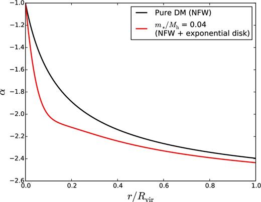
The logarithmic slope α of the mean-density profile (equation A7) as a function of the spherically averaged radial coordinate in units of the virial radius, for an NFW halo with c = 8 (black solid line) and the same halo with an additional exponential disc of mass equal to 4 per cent the total mass of the system (red solid line). Note that m*/Mh = 0.04 is the maximum stellar-to-halo mass ratio allowed by AM. The exponential disc is assumed to have a scalelength λRvir/2 ∼ 0.025Rvir, where Rvir is the halo's virial radius.
To test the accuracy of equation (A13) in recovering the correct value of rt, we have performed a numerical experiment, in which we start from the pure DM configuration in Fig. A1, we set up a range of initial conditions |$({\boldsymbol r},{\boldsymbol v})$| for the test particle and we integrate their orbits to find under what conditions the particles escape from the satellite. The experiment retains the assumptions that the satellite is on a circular orbit (i), and that the mass distributions of the host and the satellite are spherically symmetric (vii), but allow us to relax the other five assumptions (the non-sphericity of discs has a small effect on the total gravitational potential of DM plus baryons).
We compute the position of L1 by solving equation (A13) for α(Rvir; c = 8) = −2.4 and compare this result, derived from assumptions (v) and (vi), to the real position of L1 in our configuration. Then, we consider four test particles with the same initial position (they all start at L1 computed with equation A13), but with different initial velocities. Three of the four particles start on a circular orbit with |$v_{\rm orb}^2=GM_{\rm s}(r_{\rm t})/r_{\rm t}$|, where vorb is the orbital speed of P around S in an inertial frame. One corotates with |${\boldsymbol \Omega }$|, another counter rotates and the orbital plane of the third one is orthogonal to that of the binary (the third case allows us to relax assumption iii). The fourth particle starts with zero speed at the apocentre of a purely radial orbit. All four are stripped from the satellite in less than an orbital time (2π/Ω), the duration of the numerical experiment.
We then progressively lower the value of α until the particles start so close to S that they are all able to remain within the satellite. Both α = −2.4 (the value obtained from equation A7) and α = −3 (the classical Jacobi limit) correspond to initial conditions for P in between the smaller and the larger dashed circle in Fig. A1. The α below which stripping is prevented depends on the initial condition for |${\boldsymbol v}$|, but the dependence is not strong. Hence, assumptions (iii) and (iv) are likely to have a minor effect on the value of rt. Assuming α = −2.4 overestimates rt even in a pure DM configuration. So does α = −3, but only slightly. The results of a numerical experiment in which P is positioned on the inner dashed circle of Fig. A1 are qualitatively similar to those shown in the right-hand panel of Fig. A3. The only difference is that the red curve makes many more orbits around S before it escapes from the satellite.
Orbits of four test particles during one revolution of S around O. All four test particles start at the position P of First Lagrangian Point computed with equation (A13), as opposed to the true First Lagrangian Point L1, but their initial conditions for |${\boldsymbol v}$| are not the same: a particle corotates with Ω, another counter rotates with respect to Ω, a third one rotates on a plane orthogonal to the orbital plane of the two-body system and the fourth one starts on a purely radial orbit. The left- and the right-hand panels correspond to α = −2.4, that is, α(Rvir) for c = 8 and α = −3, respectively. In the first case, all the particles on circular orbits are stripped from the satellite. Only the particle on a radial orbit (green curve) is retained. In the second case, only the counter-rotating particle (red curve) escapes from the satellite. All others are retained. The units on the x- and the y-axes are host-halo virial radii.
The numerical test in Fig. A3 illustrates the limitations of our analytic approach because it shows equation (A13) with α = −2.4 from equation (A7) overestimates the real tidal radius (particles on circular orbits tend to be stripped even if they are at r < rt). However, the right-hand panel of Fig. A3 shows that rt is approximately recovered for a higher value of |α| corresponding to α = −3. In principle, this value could depend on the distance between the satellite and the central, but Fig. A2 shows that, for r/Rvir > 0.1, α should be fairly independent of radius, especially in presence of baryons (red curve).
APPENDIX B: ORBITAL TIMES
Fig. B1 displays the lookback times and corresponding redshifts for a galaxy to reach the pericentre (blue), virial radius on the way out (black) and apocentre (red) at z = 0. While the dashed lines indicate the orbital times for radial orbits, the solid lines represent orbits of typical apocentre/pericentre ratios of 5 (Ghigna et al. 1998), where we used an apocentric (tangential) velocity of 0.45 times the circular velocity at that radius. The z = 0 halo mass is 1014 M⊙, but the results vary fairly little with the halo mass (except that the virial radius is harder to reach on the way out for more massive haloes). The times to reach the pericentre and the virial radius decrease for increasing initial apocentric radius (in units of the initial Rvir), because galaxies starting at large radii travel faster through the halo. On the other hand, the time to reach the second apocentre increases for increasing first apocentric radius (in units of the initial virial radius), because there is more distance to travel outwards (e.g. from first pericentre to second apocentre), unless the initial apocentre is small, where the speed effect overcomes the distance effect.
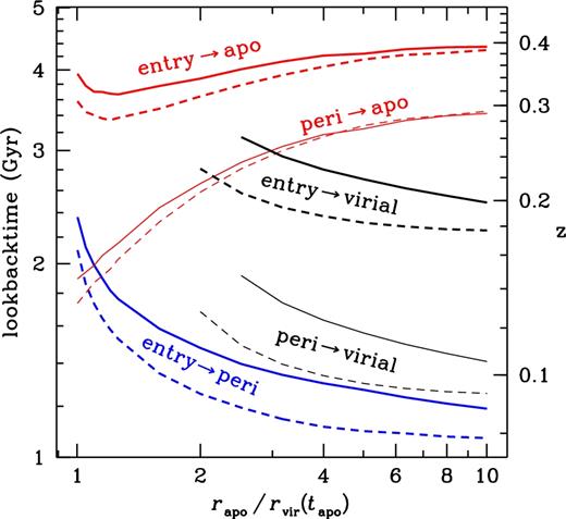
Lookback times and corresponding redshifts for galaxies to be at different locations at z = 0: pericentre (blue), virial radius on the way outwards (black) and apocentre (red), for radial orbits (dashed) and orbits of typical elongations (solid), starting the clock at cluster entry (thick) or at pericentre (thin).
APPENDIX C: FITTING PARAMETERS FOR THE SMF AND THE SMHM RELATION
In this appendix, we explain how we use the data points of Yang et al. (2012) for the local Universe and Muzzin et al. (2013) at z > 0.2 to construct the SMF n*(m*, z) that we use for AM.
| n0 | x0 | α0 | β0 |
|---|---|---|---|
| 2.39 | 11.12 | 0.228 | 3.07 |
| n1 | x1 | α1 | β1 |
| 0.501 | 4.6 × 10⁻³ | 0.133 | 0.367 |
| n0 | x0 | α0 | β0 |
|---|---|---|---|
| 2.39 | 11.12 | 0.228 | 3.07 |
| n1 | x1 | α1 | β1 |
| 0.501 | 4.6 × 10⁻³ | 0.133 | 0.367 |
| n0 | x0 | α0 | β0 |
|---|---|---|---|
| 2.39 | 11.12 | 0.228 | 3.07 |
| n1 | x1 | α1 | β1 |
| 0.501 | 4.6 × 10⁻³ | 0.133 | 0.367 |
| n0 | x0 | α0 | β0 |
|---|---|---|---|
| 2.39 | 11.12 | 0.228 | 3.07 |
| n1 | x1 | α1 | β1 |
| 0.501 | 4.6 × 10⁻³ | 0.133 | 0.367 |
Comparison between the fitted stellar mass (m*)–halo mass (Mmax) relation (dotted lines) and the original relation used in this work (solid line) at z = 0, 1 and 2. The only purpose of this fitting is to facilitate the comparison with future AM work. The best-fitting parameters are given in Table C2.
| m0 | y0 | γ0 | η0 |
|---|---|---|---|
| 10.57 | 11.69 | 3.04 | 0.417 |
| m1 | y1 | γ1 | η1 |
| −0.085 | 0.685 | −1.16 | 0.607 |
| m0 | y0 | γ0 | η0 |
|---|---|---|---|
| 10.57 | 11.69 | 3.04 | 0.417 |
| m1 | y1 | γ1 | η1 |
| −0.085 | 0.685 | −1.16 | 0.607 |
| m0 | y0 | γ0 | η0 |
|---|---|---|---|
| 10.57 | 11.69 | 3.04 | 0.417 |
| m1 | y1 | γ1 | η1 |
| −0.085 | 0.685 | −1.16 | 0.607 |
| m0 | y0 | γ0 | η0 |
|---|---|---|---|
| 10.57 | 11.69 | 3.04 | 0.417 |
| m1 | y1 | γ1 | η1 |
| −0.085 | 0.685 | −1.16 | 0.607 |
