


Abstract
We report new light curves and phase functions for nine Jupiter-family comets (JFCs). They were observed in the period 2004–2015 with various ground telescopes as part of the Survey of Ensemble Physical Properties of Cometary Nuclei as well as during devoted observing campaigns. We add to this a review of the properties of 35 JFCs with previously published rotation properties. The photometric time series were obtained in Bessel R, Harris R and SDSS r΄ filters and were absolutely calibrated using stars from the Pan-STARRS survey. This specially developed method allowed us to combine data sets taken at different epochs and instruments with absolute-calibration uncertainty down to 0.02 mag. We used the resulting time series to improve the rotation periods for comets 14P/Wolf, 47P/Ashbrook–Jackson, 94P/Russell and 110P/Hartley 3 and to determine the rotation rates of comets 93P/Lovas and 162P/Siding Spring for the first time. In addition to this, we determined the phase functions for seven of the examined comets and derived geometric albedos for eight of them. We confirm the known cut-off in bulk densities at ∼0.6 g cm−3 if JFCs are strengthless. Using a model for prolate ellipsoids with typical density and elongations, we conclude that none of the known JFCs requires tensile strength larger than 10–25 Pa to remain stable against rotational instabilities. We find evidence for an increasing linear phase function coefficient with increasing geometric albedo. The median linear phase function coefficient for JFCs is 0.046 mag deg−1 and the median geometric albedo is 4.2 per cent.
1 INTRODUCTION
Comets are believed to preserve pristine material from the epoch of planet formation. Therefore, their properties have often been studied in the search for constraints on the conditions during Solar system formation. A milestone in cometary exploration came from the European Space Agency's Rosetta mission that followed comet 67P/Churyumov–Gerasimenko through its perihelion passage in the period 2014–2016. The successful rendezvous of Rosetta with comet 67P/C-G has provided a unique ensemble of comprehensive observations which are set to fully characterize this comet. However, in order to interpret the detailed measurements from Rosetta, as well as those for other comets visited by spacecraft, we need to consider them in the context of other known comets.
One fundamental technique to derive the physical properties of comet nuclei is through their rotational light curves. Light curves can be used to extract the individual objects’ spin rates and axial ratios, which in turn can be used to constrain important properties of the comets, e.g. collisional history, density and tensile strength. Additionally, knowing the light-curve brightness variation of Jupiter-family comets (JFCs) can significantly improve the results of optical studies of JFC colour and size distributions. Despite being such a rich source of information, just a small fraction of JFCs have well-studied light curves.
There are two main techniques to derive rotational light curves from telescope observations: (1) photometric time series of bare nuclei and (2) periodic variability of coma structures of active comets (for an overview see Samarasinha et al. 2004). The former relies on the direct detection of the nucleus signal, and is expected to produce more precise results (Samarasinha et al. 2004). In order to detect the nucleus brightness variation directly, the comets need to be observed at large heliocentric distances when they are inactive. Observing the comets when they are weakly active can also allow reliable light-curve derivations, but only in the cases when the nucleus signal dominates over the coma contribution. It is also possible to derive the nucleus rotation rate of active comet nuclei, provided that they are observed with sufficient spatial resolution to distinguish the nucleus signal from that of the coma. Such observations have been performed with the Hubble Space Telescope (HST; see Lamy et al. 2004).
Additionally, comet rotations can be studied during spacecraft fly-bys. Such missions have allowed the rotational properties of three comets to be studied in greater detail: 9P (Chesley et al. 2013, and references therein), 103P (Belton et al. 2013, and references therein) and 67P (Jorda et al. 2016). The ground- and space-based telescope techniques for period derivations usually do not account for Sun–comet–Earth geometry changes and therefore produce synodic rotation periods, while the spacecraft observations allow the sidereal spin periods to be derived (see e.g. Samarasinha et al. 2004). However, the difference between the synodic and sidereal rotation periods is usually small (∼0.001 h) even for near-Earth asteroids (e.g. Pravec, Sarounova & Wolf 1996), so the synodic rotation periods are good approximations for the spin rates.
The photometric observations used to study the rotational properties of comets can also be a valuable source of information about the comets’ surface properties. The light-curve-resolved photometry allows a precise determination of the nucleus absolute magnitude. Combined with thermal infrared data, the photometric magnitude can be used to determine the geometric albedo (hereafter, albedo) of the nucleus. In some cases when the comets have been observed at multiple epochs, the photometric data can be used to derive the phase functions of the nuclei. Albedos and phase functions provide us with the opportunity to characterize the surfaces of comets (e.g. Li et al. 2013; Ciarniello et al. 2015; Fornasier et al. 2015) and to compare the icy populations in the Solar system (e.g. Belskaya et al. 2008; Masoumzadeh et al. 2017).
Previous extensive overviews of the known JFCs surface and rotation properties were published by Lamy et al. (2004), Samarasinha et al. (2004), Snodgrass, Lowry & Fitzsimmons (2006) and Lowry et al. (2008). In this work, we study the light curves and the surface properties of nine JFCs and compare them with a broad sample of JFCs with known rotational properties. This updated sample contains a collection of 37 well-studied comets, and allows us to investigate the population properties of JFCs for the first time after NASA's Deep Impact and EPOXI and ESA's Rosetta missions.
In Section 2 we review the studies of all comets, which to our knowledge have period determinations published after the last review by Snodgrass, Lowry & Fitzsimmons (2008b). This section includes Table 1 that contains the nucleus properties of the whole sample of JFCs used in this work. We describe the observations and the method for precise absolute calibration of multi-epoch time series observations in Section 3. In Section 4, we present the results from the observations of nine JFCs. After adding our comets to the rest of the JFCs with known rotational properties, we study the cumulative properties of JFCs in Section 5. Finally, Section 6 contains a summary of our results.
Summary of the properties of the comets with published rotation rates and the comets studied in this work.
| Comet | Reff (km) | Ref. Reff | Δm | Ref. Δm | a/b | Ref. a/b | Prot | Ref. Prot (h) |
|---|---|---|---|---|---|---|---|---|
| 2P | 3.95 ± 0.06 | (1) | 0.4 ± 0.04 | (1) | ≥1.44 ± 0.06 | (1) | 11.0830 ± 0.0030 | (1) |
| 6P | |$\mathrm{2.23^{+0.13}_{-0.15}}$| | (2) | 0.082 ± 0.016 | (3) | ≥1.08 | –a | 6.67 ± 0.03 | (3) |
| 7P | 2.64 ± 0.17 | (2) | 0.30 ± 0.05 | (4) | ≥1.3 ± 0.1 | (4) | |$\mathrm{7.9^{+1.6}_{-1.1}}$| | (4) |
| 9P | 2.83 ± 0.1 | (5) | 0.6 ± 0.2 | (6) | 1.89b | (5) | 41.335 ± 0.005c | (7) |
| 10P | 5.98 ± 0.04 | (8) | 0.7 | (9) | ≥1.9 | (9) | 8.948 ± 0.001 | (10) |
| 14P | 2.95 ± 0.19 | (2) | 0.37 ± 0.05 | (d) | ≥1.41 ± 0.06 | (d) | 9.02 ± 0.01 | (d) |
| 17P | 1.62 ± 0.01 | (11) | 0.30 ± 0.05 | (11) | ≥1.3 ± 0.1 | (11) | 7.2/8.6/10.3/12.8 | (11) |
| 19P | 2.5 ± 0.1 | (12) | 0.84-1.00 | (13) | 2.53 ± 0.12b | (12) | 26.0 ± 1.0 | (13) |
| 21P | 1.0 | (14) | 0.43 | (15) | ≥1.5 | (15) | 9.50 ± 0.2 | (16) |
| 22P | 2.15 ± 0.17 | (2) | 0.55 ± 0.07 | (17) | ≥1.66 ± 0.11 | (17) | 12.30 ± 0.8 | (17) |
| 28P | 10.7 ± 0.7 | (18) | 0.45 ± 0.07 | (19) | ≥1.51 ± 0.07 | (19) | 12.75 ± 0.03 | (19) |
| 31P | |$\mathrm{1.65^{+0.11}_{-0.12}}$| | (2) | 0.5 ± 0.1 | (20) | ≥1.6 ± 0.15 | (20) | 5.58 ± 0.03 | (20) |
| 36P | 2.55 ± 0.01 | (21) | 0.7 ± 0.1 | (21) | ≥1.9 ± 0.1 | (21) | ∼40 | (21) |
| 46P | 0.56 ± 0.04 | (22) | 0.38 | (22) | ≥1.4 ± 0.1 | (22) | 6.00 ± 0.3 | (23) |
| 47P | |$\mathrm{3.11^{+0.20}_{-0.21}}$| | (2) | 0.33 ± 0.06 | (d) | ≥ 1.36 ± 0.07 | (d) | 15.6 ± 0.1 | (d) |
| 48P | |$\mathrm{2.97^{+0.19}_{-0.20}}$| | (2) | 0.32 ± 0.05 | (24) | ≥1.34 ± 0.06 | (24) | 29.00 ± 0.04 | (24) |
| 49P | 4.24 ± 0.2 | (18, 25, 26) | 0.5 | (25) | ≥1.63 ± 0.07 | (25) | 13.47 ± 0.017 | (25) |
| 61P | 0.61 ± 0.03 | (27) | 0.26 | (27) | ≥1.3 | (27) | 4.9 ± 0.2 | (27) |
| 67P | 1.649 ± 0.007 | (28) | 0.4 ± 0.07 | (29) | 2.05 ± 0.06b | (28) | 12.055 ± 0.001 | ESA/Rosetta |
| 73P | 0.41 ± 0.02 | (30) | – | – | ≥1.8 ± 0.3 | (30) | 3.0 - 3.4 | (31) |
| 76P | 0.31 ± 0.01 | (27) | 0.56 | (27) | ≥1.45 | (27) | 6.6 ± 1.0 | (27) |
| 81P | 1.98 ± 0.05 | (32) | – | – | 1.67 ± 0.04 | (33) | 13.5 ± 0.1 | (34) |
| 82P | 0.59 ± 0.04 | (27) | 0.58 | (27) | ≥1.59 | (27) | ≥24 ± 5 | (27) |
| 87P | 0.26 ± 0.01 | (27) | 0.94 | (27) | ≥2.2 | (27) | 32 ± 9 | (27) |
| 92P | 2.08 ± 0.01 | (4) | 0.6 ± 0.05 | (4) | ≥1.7 ± 0.1 | (4) | 6.22 ± 0.05 | (4) |
| 93P | 2.59 ± 0.26 | (2) | 0.21 ± 0.05 | (d) | ≥1.21 ± 0.06 | (d) | |$\mathrm{18.2^{+1.5}_{-15}}$| | (d) |
| 94P | |$\mathrm{2.27^{+0.13}_{-0.15}}$| | (2) | 1.11 ± 0.09 | (d) | ≥2.8 ± 0.2 | (d) | 20.70 ± 0.07 | (d) |
| 103P | 0.58 ± 0.018 | (35) | – | – | 3.38b | (35) | 16.4 ± 0.1 | (36) |
| 110P | 2.31 ± 0.03 | (d) | 0.20 ± 0.03 | (d) | ≥1.20 ± 0.03 | (d) | 10.153 ± 0.001 | (d) |
| 121P | |$\mathrm{3.87^{+0.26}_{-0.21}}$| | (2) | 0.15 ± 0.03 | (21) | ≥1.15 ± 0.03 | (21) | |$\mathrm{10^{+8}_{-2}}$| | (21) |
| 123P | 2.18 ± 0.23 | (2) | 0.5 ± 0.1 | (d) | 1.6 ± 0.1 | (d) | – | – |
| 137P | |$\mathrm{4.04^{+0.31}_{-0.32}}$| | (2) | 0.18 ± 0.05 | (d) | 1.18 ± 0.05 | (d) | – | |
| 143P | |$\mathrm{4.79^{+0.32}_{-0.33}}$| | (2) | 0.45 ± 0.05 | (37) | ≥1.49 ± 0.05 | (18) | 17.21 ± 0.1 | (37) |
| 147P | 0.21 ± 0.02 | (27) | 0.40 | (27) | ≥1.53 | (27) | 10.5 ± 1/4.8 ± 0.2 | (27) |
| 149P | |$\mathrm{1.42^{+0.09}_{-0.10}}$| | (2) | 0.11 ± 0.04 | (d) | 1.11 ± 0.04 | (d) | – | – |
| 162P | |$\mathrm{7.03^{+0.47}_{-0.48}}$| | (2) | 0.59 ± 0.04 | (d) | ≥1.72 ± 0.06 | (d) | 32.853 ± 0.002 | (d) |
| 169P | |$\mathrm{2.48^{+0.13}_{-0.14}}$| | (2) | 0.60 ± 0.02 | (38) | ≥1.74 ± 0.03 | –a | 8.4096 ± 0.0012 | (39) |
| 209P | ∼1.53 | (40) | 0.4–0.7 | (40, 41) | ≥1.55 | (40) | 10.93 ± 0.020 | (40, 41) |
| 260P | |$\mathrm{1.54^{+0.09}_{-0.08}}$| | (2) | 0.07 | (42) | ≥1.07 | –a | 8.16 ± 0.24 | (42) |
| 322P | 0.150–0.320 | (43) | ≥0.3 | (43) | ≥1.3 | (43) | 2.8 ± 0.3 | (43) |
aCalculated with equation (5) using the brightness variation Δm.
bThe exact shape model was derived by spacecraft observations in the cited paper. The provided axial ratio is obtained by dividing the highest shape model radius to the lowest one.
cThe comet is known to increase its period and this is the minimum known value measured with sufficient precision.
dResults derived in this work.
References: (1) Lowry & Weissman (2007); (2) Fernández et al. (2013); (3) Gutierrez et al. (2003); (4) Snodgrass et al. (2005); (5) Thomas et al. (2013a); (6) Fernández et al. (2003); (7) Belton et al. (2011); (8) Lamy et al. (2009); (9) Jewitt & Luu (1989); (10) Schleicher et al. (2013); (11) Snodgrass et al. (2006); (12) Buratti et al. (2004); (13) Mueller & Samarasinha (2002); (14) Tancredi et al. (2000); (15) Mueller (1992); (16) Leibowitz & Brosch (1986); (17) Lowry & Weissman (2003); (18) Lamy et al. (2004); (19) Delahodde et al. (2001); (20) Luu & Jewitt (1992); (21) Snodgrass et al. (2008b); (22) Boehnhardt et al. (2002); (23) Lamy et al. (1998a); (24) Jewitt & Sheppard (2004); (25) Millis, A'Hearn & Campins (1988); (26) Campins et al. (1995); (27) Lamy et al. (2011); (28) Jorda et al. (2016); (29) Tubiana et al. (2008); (30) Toth & Lisse (2006); (31) Drahus et al. (2010); (32) Sekanina et al. (2004); (33) Duxbury et al. (2004); (34) Mueller et al. (2010a); (35) Thomas et al. (2013b); (36) Meech et al. (2009); (37) Jewitt, Sheppard & Fernndez (2003); (38) Warner (2006); (39) Kasuga et al. (2010); (40) Howell et al. (2014); (41) Schleicher & Knight (2016); (42) Manzini et al. (2014); 43 Knight et al. (2016).
2 OVERVIEW OF THE KNOWN JFC ROTATION PROPERTIES
The aim of this study is to combine the newly obtained nuclei properties with those from previous works in order to analyse the bulk properties of the expanded sample of JFCs. Previously, the collective rotational properties of JFCs were studied by Lamy et al. (2004), Samarasinha et al. (2004) and Snodgrass et al. (2006). We expand their samples to include the cometary nuclei whose rotations were derived since then, and complement them with the newly obtained results from this work. Table 1 contains the properties of all considered comets together with the sources of all known parameters. However, the sections below focus in detail only on the comets with updates since the reviews in Lamy et al. (2004) and Snodgrass et al. (2006), including the unpublished HST results quoted in Lamy et al. (2004) that were revised by Lamy et al. (2011).
In addition to the rotational properties, we also review below the published size and shape estimates of the considered comets. While photometric light curves can be used to determine nucleus shapes, they do not provide absolute sizes. For those comets visited by spacecraft, the dimensions of shape models are directly measured. Radar data also provide absolute sizes for the comets with close approaches to the Earth. Combined thermal infrared and optical (reflected sunlight) data allow the albedo and cross-sectional area of the body (and hence an effective radius) to be determined. For those objects with only photometric data, the nucleus size can be estimated by assuming a geometric albedo of typically 4 per cent. The most recent reviews of comet sizes from visible photometry and thermal IR Spitzer photometry are given by Snodgrass et al. (2011) and Fernández et al. (2013), respectively.
2.1 Jupiter-family comets with recently updated rotation rates
2.1.1 2P/Encke
Comet 2P/Encke is among the comets with the shortest known orbital periods, 3.3 yr, which has allowed different observers to study its properties over multiple apparitions. Its relatively small heliocentric distance at aphelion of 4.1 au allows the comet to stay mildly active at almost all times, which has hindered the direct observation of the comet's nucleus. Nevertheless, 2P is one of the best-studied JFCs, having well-constrained spin rate, rotation changes, colour, albedo and phase function. All of the earlier works leading to today's relatively good understanding of 2P are thoroughly described in Lamy et al. (2004) and Lowry & Weissman (2007). Newer papers have added spectroscopy of the nucleus (Tubiana et al. 2015) and a study of the aphelion activity of this comet (Kelley et al., in preparation). Here, we provide an outline of the most important results on the nucleus shape and rotation rate.
The earliest attempts to determine the rotational light curve of 2P came from Jewitt & Meech (1987). Their time series optical photometry suggested a most likely period of 22.43 ± 0.08 h. A later study by Luu & Jewitt (1990) led to a best-fitting period of 15.08 ± 0.08 h, although both studies note that alternative periods were also consistent with their data. Fernández (2000) used thermal infrared time series data to confirm the 15.08 h period. A large data set of observations between 2001 July and 2002 September when 2P was close to perihelion was used by Fernández et al. (2005) to determine that the comet's synodic period was either 11.079 ± 0.009 h or 22.158 ± 0.012 h. Fernández et al. (2005) also discussed that these periods are not compatible with the spin rates found by Jewitt & Meech (1987) and Luu & Jewitt (1990).
Belton et al. (2005) compiled the available optical and infrared photometry and reached the conclusion that the nucleus of 2P is in a complex or excited rotation state. According to this analysis, the nucleus precesses about the total angular momentum vector with a period 11.8 h and oscillates around the long axis with period 47.8 h.
Lowry & Weissman (2007) added new optical data sets collected in 2002 October, just a few weeks apart from some of the observations in Fernández et al. (2005). This allowed Lowry & Weissman (2007) to combine data from the two studies and to derive an effective radius 3.95 ± 0.06 km, an axial ratio of 1.44 ± 0.06 and a rotation period of 11.083 ± 0.003 h.
2P was later observed during the following aphelion, and the light curves obtained suggested that the spin period increases by ∼4 min per orbit (Mueller, Samarasinha & Fernandez 2008; Samarasinha & Mueller 2013).
The early nucleus size estimates of ≤ 2.9 km (Campins 1988, we use effective radius to characterize the nucleus size hereafter) and 2.8 ≤ reff ≤ 6.4 km (Jewitt & Meech 1987; Luu & Jewitt 1990) were confirmed by the later estimate of 2.4 ± 0.3 km by Fernández (2000). Comet 2P was also observed with radar during two apparitions (Kamoun et al. 1982; Harmon & Nolan 2005). The data from Harmon & Nolan (2005) confirmed a period of ∼11 h and excluded the longer periods of ∼15 and ∼22 h. Harmon & Nolan (2005) combined the radar data with previous infrared observations and obtained a solution for 2P's shape with an effective radius of 2.42 km and an axial ratio of 2.6.
Fernández (2000) also managed to obtain the phase function of 2P with phase coefficient 0.06 mag deg−1 (in the range between 0° and 106°) as well as a relatively high visual geometric albedo of 5 ± 2 per cent.
2.1.2 9P/Tempel 1
9P/Tempel 1 was the target for two NASA missions: Deep Impact and Stardust-NExT. It was also extensively observed from ground during the supporting campaigns (Meech et al. 2005, 2011a).
Multiple authors studied the size, shape and rotation rate of 9P before the Deep Impact fly-by (e.g. Lowry et al. 1999; Weissman et al. 1999; Lamy et al. 2001; Lowry & Fitzsimmons 2001; Fernández et al. 2003). A detailed overview of their contributions can be found in Lamy et al. (2004).
The two fly-bys provided sufficient information to determine the size of the nucleus with good precision. The mean radius of the shape model after the Deep Impact fly-by was estimated as 3.0 ± 0.1 km, with axes of 7.6 and 4.9 km, and an axial ratio a/b = 1.55 (A'Hearn et al. 2005). Thomas et al. (2013a) combined the data sets from the two spacecraft and obtained a radius of 2.83 ± 0.1 km. They reported a shape model with radii between 2.10 and 3.97 km, which gives an axial ratio a/b = 1.89.
The two fly-bys combined with the ground observing campaigns gave an insight into the rotation of 9P. Belton et al. (2011) analysed multiple available data sets and determined that 9P had the following sidereal rotation periods: 41.335 ± 0.005 h before the 2000 perihelion passage; 41.055 ± 0.003 h between the perihelion passages in 2000 and 2005; 40.783 ± 0.006 h from the Deep Impact photometry slightly before the 2005 perihelion passage, and 40.827 ± 0.002 h in the period 2006–2010. Chesley et al. (2013) updated their work and concluded that 9P/Tempel 1 spun up by either 12 or 17 min during perihelion passage in 2000 and by 13.49 ± 0.01 min during the perihelion passage in 2005.
2.1.3 10P/Tempel 2
10P/Tempel 2 is one of the largest known JFCs. It is also known to be only weakly active at perihelion. The combination of these two factors has allowed its nucleus to be observed with very small coma contribution both at aphelion and perihelion, making 10P one of the best-studied comets.
A series of works have determined that 10P has a spheroidal shape with dimensions a = 8–8.15 km and b = c = 4–4.3 km (axial ratio of 1.9), albedo AR = 2.4 ± 0.5 per cent and rotation period about 9 h (Sekanina 1987; Jewitt & Luu 1989; A'Hearn et al. 1989). A detailed summary of the works that have estimated the size of the nucleus of 10P can be found in Lamy et al. (2004). Lamy et al. (2009) used HST photometry to determine a nucleus radius of 5.98 ± 0.04 km.
10P is one of the first comets observed to change its spin rate on orbital time-scales. It is progressively slowing down by ∼16 s per perihelion passage (Mueller & Ferrin 1996; Knight et al. 2011, 2012). The most recent analysis by Schleicher, Knight & Levine (2013) led to the conclusions that 10P has a prograde rotation with a period of 8.948 ± 0.001 h, and that the rate of spin-down has decreased over time, most likely in accordance with the known decrease in water production by the comet since 1988.
2.1.4 19P/Borrelly
The nucleus of comet 19P/Borelly was studied using HST images by Lamy, Toth & Weaver (1998b). Their analysis suggested a rotation rate of 25.0 ± 0.5 h and dimensions of 4.4 ± 0.3 km × 1.8 ± 0.15 km, assuming an albedo of 4 per cent. The comet was observed during five nights in 2000 July/August at the CTIO 1.5-m telescope (Mueller & Samarasinha 2002). These data yielded a light curve with period 26.0 ± 1 h and a large light-curve variation – between 0.84 and 1.0 mag.
On 2001 September 22, just eight days after 19P passed perihelion, the NASA-JPL Deep Space 1 Mission had a fly-by of the comet (Soderblom et al. 2002). Using the encounter images, Buratti et al. (2004) determined that the nucleus has a radius of 2.5 ± 0.1 km and axes 4.0 ± 0.1 km and 1.58 ± 0.06 km. Dividing these two values yields an axial ratio a/b = 2.53 ± 0.12.
HST/STIS observations were conducted in parallel to the Deep Space 1 encounter (Weaver, Stern & Parker 2003). They could not be used to derive an independent measure of the nucleus rotation rate but were in agreement with the previous period measurement from Lamy et al. (1998b). Mueller & Samarasinha (2002) collected all available ground-based data from 2000 and the HST data from 2001 and improved the period by one order of magnitude. They narrowed down the possible periods to three values P = 1.088 ± 0.003 d, P = 1.108 ± 0.002 d and P = 1.135 ± 0.003 d, which were consistent with the initial period of P = 1.08 ± 0.04 d from Mueller & Samarasinha (2002) (Mueller et al. 2010b). These authors continued studying the comet with observations from the SOAR telescope in Chile in 2014 September/October (Mueller & Samarasinha 2015). These new data were used in an attempt to choose between the three possible rotation periods as well as to look for activity-induced spin changes of the nucleus during the two apparitions since the last observations. The most likely period was 1.209 d (29.016 h) but 1.187 d (28.488 h) could not be excluded (Mueller & Samarasinha 2015). The newly derived period suggested that the rotation of 19P slows down by approximately 20 min per orbit (Mueller & Samarasinha 2015).
2.1.5 61P/Shajn–Schaldach
Lowry, Fitzsimmons & Collander-Brown (2003) used snapshot observations of the nucleus of 61P (in non-photometric conditions) to determine a radius of 0.92 ± 0.24 km. Lamy et al. (2011) observed the comet at heliocentric distance 2.96 au (inbound) and determined a mean nucleus radius of 0.61 ± 0.03 km and axial ratio a/b ≥ 1.3. Their partial rotational light curve suggested a few possible periods, but the shortest one of them, 4.9 ± 0.2 h was considered as most likely (Lamy et al. 2011).
2.1.6 67P/Churyumov–Gerasimenko
Comet 67P/Churyumov–Gerasimenko was selected as the backup target for the Rosetta mission after the 2003 launch of the mission had to be postponed due to a failure of the Ariane rocket (Glassmeier et al. 2007). The comet was observed in detail during only two apparitions before the rendezvous in 2014 August.
The rotation period of 67P was first constrained to ∼12 h by HST observations in 2003 March, soon after its perihelion passage in 2002 September (Lamy et al. 2006). After the comet moved to greater heliocentric distances and its activity was quenched, it was possible to directly observe the nucleus from ground and to determine the spin rate with greater precision. Lowry et al. (2012) combined all available ground observations (Lowry et al. 2006; Tubiana et al. 2008, 2011) and determined the sidereal rotation period of the nucleus to be P = 12.761 37 ± 0.000 06 h. Mottola et al. (2014) revised the period before the second perihelion passage in 2009, and set it to P = 12.761 29 ± 0.000 05 h.
The next period determination was done with measurements from the Rosetta camera OSIRIS in 2014 March (Mottola et al. 2014). The new period of the comet was determined as P = 12.4043 ± 0.0007 h and suggested that the nucleus had spun up by 1285 s (∼21 min; Mottola et al. 2014).
OSIRIS continued monitoring the temporal evolution of the rotation rate of 67P throughout the extent of the mission (Jorda et al. 2016). The perihelion measurements of the orientation of the comet's rotational axis determined an excited rotational state with period of 11.5 ± 0.5 d and an amplitude of 0|$_{.}^{\circ}$|15 ± 0|$_{.}^{\circ}$|03 (Jorda et al. 2016). They determined a rotation period of 12.4041 ± 0.0001 h, which stayed constant from 2014 early July until the end of 2014 October. After that the rotation rate slowly increased to 12.4304 h until 2015 May 19, when it started dropping to reach 12.305 h just before perihelion on 2015 August 10 (Jorda et al. 2016).
According to the Rosetta measurements made available by ESA,1 the rotation rate continued decreasing until 2016 February, and at the end of the mission, the sidereal period of 67P was 12.055 h (ESA provided no uncertainty on this value). These measurements imply that 67P spun up by 1257 s (∼21 min) during its latest perihelion passage (2014–2016). This period change is similar to the change of 1285 s measured by Mottola et al. (2014), which suggests that the comet spins up with a rate of approximately 21 min per orbit.
The overall spin evolution of 67P is in very close agreement with the activity model of Keller et al. (2015). According to their analysis, the sign of the rotation period change is determined by the nucleus shape, while the magnitude of the change is controlled by the activity of the comet.
Rosetta measured the precise dimensions of the bilobate nucleus of 67P (Sierks et al. 2015). The overall dimensions along the principal axes are (4.34 ± 0.02) × (2.60 ± 0.02) × (2.12 ± 0.06) km, with the two lobes being 4.10 × 3.52 × 1.63 km and 2.50 × 2.14 × 1.64 km (Jorda et al. 2016). Using the longest and the shortest axes of the comet, we calculated an axial ratio a/b = 2.05 ± 0.06.
The mean radius derived from the shape model of 67P is 1.743 ± 0.007 km. The area equivalent radius and the volume equivalent radius are 1.93 ± 0.05 km and 1.649 ± 0.007 km, respectively (Jorda et al. 2016).
2.1.7 73P/Schwassmann–Wachmann 3
Comet 73P/Schwassmann–Wachmann had a strong outburst in 1995 September (Crovisier et al. 1995) which was accompanied by a split-up into at least four pieces (Bohnhardt et al. 1995; Scotti et al. 1996). The remnants of the 73P nucleus were detected during the subsequent apparitions. The largest one of them is fragment C, which was estimated to have a radius of 0.5 km (Toth, Lamy & Weaver 2005; Nolan et al. 2006; Toth & Lisse 2006).
In 2006, the comet approached Earth to less than 1 au and provided an excellent opportunity for different observers to study the light curve of fragment C. Toth et al. (2005) and Toth & Lisse (2006) used HST data to determine the dimensions of fragment C. Assuming an albedo of 0.04 and a linear phase coefficient of 0.04 mag deg−1 for the R band, they obtained an effective radius of 0.41 ± 0.02 km. The derived light curve suggested an elongated body with axes 0.57 ± 0.08 km and 0.31 ± 0.02 km, which results in a minimum axial ratio a/b ≥ 1.8 ± 0.3 (Toth & Lisse 2006).
Drahus et al. (2010) collected all of the reported light curves (Farnham 2001; Nolan et al. 2006; Storm et al. 2006; Toth & Lisse 2006), and added a further estimate of the spin rate using variations in the production rates of the HCN molecule from sub-mm observations. Their analysis showed that 73P-C had a stable rotation during the 21-d observing campaign in 2006 May and narrowed down the possible periods to 3.392, 3.349 or 3.019 h. Since none of these values could be excluded, Drahus et al. (2010) concluded that the rotation period of 73P-C was between 3.0 and 3.4 h during the duration of their observing campaign. This is the fastest known rotation period of a JFC and its stability against rotational splitting suggests that 73P-C has a bulk tensile strength of at least 14–45 Pa (Drahus et al. 2010), or that it has a higher than expected density (see Section 5.3). Given that 73P has previously split, and continues to fragment (Williams 2017), it is most likely at the very limit of stability.
2.1.8 76P/West–Kohoutek–Ikemura
Tancredi et al. (2000) observed the nucleus of 76P and estimated a radius of 1.3 km. However, the authors note that the collected photometric measurements of the nucleus brightness had a large scatter that makes the radius value uncertain. Lamy et al. (2011) obtained a partial light curve of the comet with most likely period of 6.6 ± 1.0 h and brightness variation of 0.56 mag which corresponds to an axial ratio a/b ≥ 1.45. They estimated the nucleus radius to be 0.31 ± 0.01 km (Lamy et al. 2011).
2.1.9 81P/Wild 2
Comet 81P/Wild 2 was the primary target of the sample-return mission Stardust. The observations of 81P before 2004 provided an estimate of its size (summarized in Lamy et al. 2004). During the Stardust fly-by in 2004 January, the instruments on board revealed the shape of the nucleus as well as great details from the surface. Duxbury, Newburn & Brownlee (2004) used the obtained images to model the nucleus as a triaxial ellipsoid with radii 1.65 × 2.00 × 2.75 km ± 0.05 km, while the model of Sekanina et al. (2004) provided an effective radius of 1.98 km.
The rotation rate of the comet remained unknown until 81P was observed at perigee in 2010 March/April (Mueller et al. 2010a). Their narrow-band filter photometry revealed a periodic variation in the CN features of the coma with a period of 13.5 ± 0.1 h.
2.1.10 82P/Gehrels 3
The radius of 82P was estimated to be Reff < 3.0 km (Licandro et al. 2000) or Reff = 2.0 km (Tancredi et al. 2000). However, 82P shows signs of activity all along its orbit (e.g. Licandro et al. 2000), and these values are therefore most likely influenced by the presence of coma.
Lamy et al. (2011) obtained a partial light curve with a rotation period P = 24 ± 5 h. However, the light curve is poorly sampled and this result most likely corresponds to a lower limit of the comet's rotation period (Lamy et al. 2011). The authors used the same data set to derive a mean radius Reff = 0.59 ± 0.04 km and axial ratio a/b ≥ 1.59.
2.1.11 87P/Bus
The attempts to determine the size of the nucleus of 87P resulted in the following upper limits: rn ≤ 0.8 km (Lowry & Fitzsimmons 2001), rn ≤ 0.6 km (Lowry et al. 2003) and rn < 3.14–3.42 (Meech, Hainaut & Marsden 2004).
Lamy et al. (2011) analysed a partial HST light curve of 87P and determined a most likely period of 32 ± 9 h, a mean radius of 0.26 ± 0.01 km and an axial ratio a/b ≥ 2.2.
2.1.12 103P/Hartley 2
103P/Hartley 2 was extensively studied during the EPOXI fly-by on 2010 November 4, and has been the target of multiple ground observations due to its favourable observing geometry during close approaches to Earth. The first determinations of its radius rn = 0.58 km came from Jorda et al. (2000) but was later revised to rn = 0.71 ± 0.13 km (Groussin et al. 2004). This result was consistent with the upper limits set by Licandro et al. (2000), Lowry et al. (2003), Lowry & Fitzsimmons (2001) and Snodgrass et al. (2008b). In preparation for the EPOXI mission, Lisse et al. (2009) used Spitzer to measure an effective radius of 0.57 ± 0.08 km. This value was practically the same as the mean radius of 0.580 ± 0.018 km measured with the in situ instruments of EPOXI (Thomas et al. 2013b). The shape model presented in Thomas et al. (2013b) results in an estimated diameter range for the nucleus of 0.69–2.33 km. We divided the two extreme diameter values to obtain an axial ratio a/b = 3.38.
The rotation period of 103P was studied in detail using the EPOXI data as well as the extensive support observations from ground. It was established that the nucleus is slowing down during the perihelion passage and that it is in a non-principal axis rotation (Jehin et al. 2010; Samarasinha et al. 2010, 2011, 2012; A'Hearn et al. 2011; Drahus et al. 2011; Harmon et al. 2011; Knight et al. 2011, 2015; Meech et al. 2011b; Belton et al. 2013). The EPOXI light curve suggested several periodicities ranging from 17 to 90 h (A'Hearn et al. 2011; Belton et al. 2013), which were used to understand the complex rotation of the nucleus (A'Hearn et al. 2011; Samarasinha et al. 2012; Belton et al. 2013). The ground observations between 2009 April and 2010 December monitored the change in the strongest periodicity of ∼18 h, which corresponds to the precession of the long axis of the nucleus around the angular momentum vector (Meech et al. 2011b). Over the period covered by the campaign, the rotation rate increased by ∼2 h, from 16.4 ± 0.1 h (Meech et al. 2009, 2011b) to 18.4 ± 0.3 or 19 h (Jehin et al. 2010).
2.1.13 147P/Kushida–Muramatsu
147P is among the smallest known JFC nuclei. Regarding the orbit class of this comet, Ohtsuka et al. (2008) showed that 147P is a quasi-Hilda comet, which underwent a temporary satellite capture by Jupiter between 1949 and 1961. Tancredi et al. (2000) reported a nucleus radius of 2.3 km but noted that the measurement is uncertain. Lowry et al. (2003) reported rn ≤ 2.0 km after a non-detection at heliocentric distance of 4.11 au. Lamy et al. (2011) derived a complete but poorly sampled light curve, which suggested that the rotation period of 147P was either 10.5 ± 1 h or 4.8 ± 0.2 h, where the former period is slightly favoured by the obtained periodogram. They estimate a radius of 0.21 ± 0.02 km and an axial ratio a/b ≥ 1.53.
2.1.14 169P/NEAT
Comet 169P/NEAT was discovered as asteroid 2002 EX12 by the NEAT survey in 2002. Later it was designated as 169P/NEAT due to the detection of cometary activity (Warner & Fitzsimmons 2005). Due to its albedo of 0.03 ± 0.01 (DeMeo & Binzel 2008) and its weak activity level, 169P is considered to be a transition object on its way to becoming a dormant comet.
Warner (2006) reported the first rotational light curve of 169P with a double-peaked period 8.369 ± 0.05 h and peak-to-peak amplitude Δm = 0.60 ± 0.02 mag. Later, Kasuga, Balam & Wiegert (2010) observed the comet with a much larger (1.85-m) telescope and separated the nucleus brightness from the slight coma contribution. Therefore, their derived light-curve period of 8.4096 ± 0.0012 h, photometric range Δm = 0.29 ± 0.02 mag and consequent effective radius of 2.3 ± 0.4 km are more reliable measures of the nucleus properties. However, the presence of coma during the observations done by Warner (2006) would suppress the light-curve amplitude. Therefore, the higher amplitude measured by Warner (2006) must instead be the result of a more elongated shape, measured at a different aspect than Kasuga et al. (2010), unless the coma is highly variable on a time-scale shorter than the spin period. However, due to the weak levels of activity present in this comet, this level of variability is unrealistic and we adopt the larger implied axial ratio limit from the Warner (2006) data.
Fernández et al. (2013) determined an effective radius of |$\mathrm{2.48^{+0.13}_{-0.14}}$| km for 169P using Spitzer mid-infrared data.
2.1.15 209P/LINEAR
Hergenrother (2014) observed 209P and found its rotation rate to be either 10.93 or 21.86 h. In 2014 May, the comet had an exceptionally close approach to Earth (0.6 au) which provided an opportunity for detailed studies of its intrinsically faint nucleus. Howell et al. (2014) used the Arecibo and Goldstone planetary radar systems to directly measure the nucleus to be 3.9 × 2.7 × 2.6 km in size, and calculated an effective radius of ∼1.53 km. These observations ruled out the longer period by Hergenrother (2014) since the measured rotational velocities were too fast for the longer period.
Schleicher & Knight (2016) also observed 209P during its perigee in 2014 May. They used images obtained mainly with the 4.3-m Discovery Channel Telescope to study the coma and the nucleus of the comet. They used a small aperture with fixed projected size of 312 km, minimizing the coma contribution so that the estimated nucleus fraction of the obtained light was 52–69 per cent (Schleicher & Knight 2016). Their light curve was consistent with the two periods from Hergenrother (2014). However, Schleicher & Knight (2016) preferred the shorter value, 10.93 h, since it also agreed with the radar observations. Schleicher & Knight (2016) reported that their light curve had a different shape than the one in Hergenrother (2014). Additionally, they measured variation of 0.6–0.7 mag, which is larger than the prediction of 0.4 mag based on the radar measurements. These differences can be explained by a possible interplay between shape and viewing geometry as well as albedo effects (Schleicher & Knight 2016). Despite these discrepancies, all three investigations agree on the spin period of 10.93 h.
2.1.16 260P/McNaught
260P was discovered in 2012, and the most reliable estimate of its effective radius to date is |$1.54^{+0.09}_{-0.08}$| km (Fernández et al. 2013). Its rotational characteristics were studied by Manzini et al. (2014) with ground photometric observations while the comet was around perihelion in 2012 and 2013. Manzini et al. (2014) used coma structures to constrain the pole orientation of the comet, but they were unable to use the coma morphology to derive a rotational period. Instead, the comet's light curve was obtained by measuring the coma brightness with apertures larger than the seeing disc but small enough to include only contribution from the coma at a distance up to 2000–2500 km from the surface (Manzini et al. 2014). The resulting light curve had a variation of 0.07 mag and could be phased with a few possible periods, best summarized as 8.16 ± 0.24 h.
While the method used in Manzini et al. (2014) has been used successfully to derive other rotations periods of comets with weak jet activity (e.g. Reyniers et al. 2009), we regard the results on 260P with caution. It is very likely that the coma contribution in the selected apertures dilutes the received nucleus signal and dampens the possible variation caused by rotation. Therefore, the limit on the nucleus elongation derived from the brightness variation is a weak constraint on the nucleus shape.
2.1.17 322P/SOHO 1
Comet 332P/SOHO 1 was discovered by SOHO as C/1999 R1, but after it was identified again in the SOHO fields during the following apparitions (Hoenig 2005), it became the first SOHO-discovered comet with conclusive orbital periodicity. The observations of 322P during four consecutive apparitions displayed no clear signatures of a coma or tail and showed a nearly identical asymmetrical heliocentric light curve, implying repeated activity at similar levels each orbit (Lamy et al. 2013).
Despite its comet-like orbit with Tisserand parameter with respect to Jupiter of 2.3, the unusual properties of 322P suggest that it has asteroidal rather than cometary origin (Knight et al. 2016). Their optical light curve indicates a fast rotation rate of 2.8 ± 0.3 h and photometric range of ≳ 0.3 mag. These figures imply a density of >1000 kg m−3, which strengthens the argument for asteroidal origin (Knight et al. 2016). This density is significantly higher than the typical values of other known comets but is typical for asteroids (see Section 5.3). Additionally, the colour of 322P is indicative of V- and Q-type asteroids, and its albedo (estimated to be between 0.09 and 0.42) is higher than the albedos measured for any other comet (Knight et al. 2016). These, together with the very low activity of the nucleus, indicate the possibility that 322P is an asteroid that becomes active when very close to the Sun. However, since no other comet nucleus has been studied so close to the Sun, it is not excluded that it has a cometary origin, but proximity to the Sun has changed the properties of its surface (Knight et al. 2016).
2.2 Comets with new rotation rates derived in this work
2.2.1 14P/Wolf
The first attempt to find the size of the nucleus of comet 14P/Wolf resulted in an effective radius of 1.3 km (Tancredi et al. 2000). However, the authors classified the estimate as poor due to the large scatter in the data points. Lowry et al. (2003) determined a radius of 2.3 km using snapshots of the comet at large heliocentric distance (3.98 au). The most recent value for the comet effective radius is 2.95 ± 0.19 km, obtained within the Survey of Ensemble Physical Properties of Cometary Nuclei (SEPPCoN) (Fernández et al. 2013). SEPPCoN used Spitzer infrared photometry to measure sizes, and should be more reliable than visible photometry from earlier ground-based surveys.
Snodgrass, Fitzsimmons & Lowry (2005) obtained time series of the bare nucleus of 14P on 2004 January 20 and 21 with the New Technology Telescope (NTT) in La Silla. The observations showed a clear brightness variation of the nucleus with a period of 7.53 ± 0.10 h. The peak-to-peak variation of the light curve was 0.55 ± 0.05 mag, which corresponds to an axial ratio a/b ≥ 1.7 ± 0.1. The mean absolute magnitude of the time series was 22.281 ± 0.007, which suggested an effective radius 3.16 ± 0.01, assuming an albedo of 4 per cent (Snodgrass et al. 2005).
In Section 4.1, we provide the results from our light-curve analysis. We combined the re-analysed data from 2004 with a SEPPCoN data set from 2007 in order to improve the light curve of the comet and to derive its phase function.
2.2.2 47P/Ashbrook–Jackson
The early estimates of the nucleus size of 47P from photometric observations close to aphelion determined an effective radius Reff = 3.0 km (Licandro et al. 2000) and Reff = 2.9 km (Tancredi et al. 2000). Snodgrass et al. (2006) and Snodgrass et al. (2008b) observed the nucleus in 2005 and 2006 at large heliocentric distance close to aphelion and estimated Reff = 2.96 ± 0.05 km. However, their photometric comet profiles showed signatures of activity, and therefore this estimate was considered an upper limit of the nucleus size. Lamy et al. (2011) used HST observations of the active nucleus of 47P to determine a mean effective radius of 2.86 ± 0.08 km. The most recent effective radius measurement of |$\mathrm{3.11^{+0.20}_{- 0.21}}$| km was obtained within the SEPPCoN survey (Fernández et al. 2013).
Lamy et al. (2011) derived a partial light curve with multiple possible periods. Analysing the periodogram, they suggested that the rotation period of the comet is ≥16 ± 8 h. Both Snodgrass et al. (2008b) and Lamy et al. (2011) attempted to constrain the phase function of 47P by combining all mentioned photometric observations. While the analysis of Snodgrass et al. (2008b) clearly suggested a linear phase function with a slope β = 0.083 mag deg−1, Lamy et al. (2011) showed that a less steep phase function similar to that of 19P/Borelly (0.072 ± 0.020 per cent; Li et al. 2007b) is also possible.
In Section 4.2, we show the result from our analysis of the data from Snodgrass et al. (2008b) complemented by a new data set obtained in 2015. We determined the light curve and the phase function of 47P, but the derived results need to be considered with caution since the comet was active during both observing runs.
2.2.3 93P/Lovas
Comet 93P/Lovas was one of the targets of the SEPPCoN survey. Its effective radius Reff = 2.59 ± 0.26 km was derived from Spitzer thermal emission observations (Fernández et al. 2013).
Our optical time series observations are presented in Section 4.3. Despite the weak activity detected on the frames, we attempted to constrain the comet's rotation light curve.
2.2.4 94P/Russell 4
Tancredi et al. (2000) tried to estimate the effective radius of 94P. However, at the time of the observations, the comet exhibited slight activity and the absolute magnitude measurements of the nucleus had large scatter. Therefore, Tancredi et al. (2000) considered their effective radius estimate of 1.9 km as uncertain and estimated the error bars of the measurement to be between ± 0.6 and ± 1 mag.
Snodgrass et al. (2008b) observed the comet during four nights in 2005 July at heliocentric distance 4.14 au, outbound. The analysis pointed to a nucleus with effective radius of 2.62 ± 0.02 km and a light curve with period ∼33 h (Snodgrass et al. 2008b). The peak-to-peak variation of the light curve was 1.2 ± 0.2 mag, implying axial ratio a/b ≥ 3.0 ± 0.5. Their nucleus size estimate Reff = 2.62 ± 0.02 km is in a good agreement with the SEPPCoN Spitzer data from Fernández et al. (2013), who reported an effective radius of |$2.27^{+0.13}_{-0.15}$| km.
In Section 4.4, we present two additional data sets from 2007 and 2009 with time series photometry of 94P. They allowed us to determine the rotational light curve and the phase function of the comet.
2.2.5 110P/Hartley 3
110P/Hartley 3 was observed with HST on 2000 November 24 at heliocentric distance of 2.58 au, inbound (Lamy et al. 2011). The data yielded an estimate of the effective radius of the nucleus Reff = 2.15 ± 0.04 km and a light curve with period 9.4 ± 1 h. The peak-to-peak amplitude of the obtained light curve was 0.4 mag, which suggested an axial ratio a/b ≥ 1.30.
In Section 4.5, we analyse a further data set from 2012 which our team had obtained in order to derive the comet's phase function. We used the data to derive a precise phase function of the comet as well as to constrain better the light curve of 110P.
2.2.6 123P/West–Hartley
Tancredi et al. (2000) estimated a radius of 2.2 km for the nucleus of comet 123P/West–Hartley. However, the authors consider this result as very uncertain as the individual photometric measurements of the comet nucleus displayed a large scatter. The SEPPCoN mid-infrared observations of 123P yielded an effective radius of 2.18 ± 0.23 km (Fernández et al. 2013).
In Section 4.6, we present the results from our analysis of a SEPPCoN data set from three observing nights in 2007. The comet was very faint (mr = 23.3 ± 0.1 mag) and weakly active during the observations, which significantly obstructed the light-curve analysis.
2.2.7 137P/Shoemaker–Levy 2
Licandro et al. (2000) observed 137P at heliocentric distance 4.24 au and determined an effective radius of 4.2 km and a brightness variation of 0.4 mag. As described in Licandro et al. (2000), their observations suffered from different technical problems, and therefore this result is uncertain. Lowry et al. (2003) obtained a radius ≤3.4 km from observations of the still active nucleus of 137P at heliocentric distance 2.29 au. Tancredi et al. (2000) observed the comet at 5 au from the Sun and estimated the effective nucleus radius to be 2.9 km. Finally, Fernández et al. (2013) targeted the comet as part of SEPPCoN and measured an effective radius of |$4.04^{+0.31}_{-0.32}$| km.
Snodgrass et al. (2006) obtained time series photometry from one night on NTT/EMMI in La Silla. The data did not show brightness variation within the 3 h of the observations and could not be used to determine the rotation rate of the nucleus. However, Snodgrass et al. (2006) used these frames to estimate the nucleus radius as 3.58 ± 0.05 km. We added two further nights of time series obtained within SEPPCoN to the one night reported in Snodgrass et al. (2006) and we used the combined data set in an attempt to characterize the phase function and the rotational properties of the comet (Section 4.7).
2.2.8 149P/Mueller 4
149P/Mueller was among the SEPPCoN targets. The Spitzer observations revealed a nucleus with an effective radius of |$1.42^{+0.09}_{-0.10}$| km (Fernández et al. 2013). To our knowledge, no previous light curves of this comet are available.
In Section 4.8, we present an analysis of the optical observations taken as part of SEPPCoN. We use the data to derive the phase function of the comet and to place constraints on its shape and albedo.
2.2.9 162P/Siding Spring
Comet 162P was discovered as asteroid 2004 TU12 but was later identified as a comet since it shows weak intermittent activity (Campins et al. 2006, and references therein).
Fernandez et al. (2006) analysed its thermal emission from NASA's Infrared Telescope Facility in 2004 December during the same apparition. Their measurements suggested a remarkably large nucleus with an effective radius of 6.0 ± 0.8 km (Fernandez et al. 2006). 162P was also observed within SEPPCoN. The Spitzer mid-infrared observations from 2007 provided a more precise estimate of the effective radius, |$R_{\mathrm{eff}}=7.03^{+0.47}_{-0.48}$| km (Fernández et al. 2013).
There are no published rotational light curves of the nucleus of 162P to our knowledge. However, there is a well-sampled light curve with period Prot ∼ 33 h by the amateur observatory La Cañada.2 Those data were taken in 2004 November, just a month after the discovery of the comet.
In Section 4.9, we analyse two time series data sets from 2007 and 2012. These data allow us to derive the phase function of 162P and to estimate its rotation period at two different epochs.
2.3 Other objects
There are a number of objects that are not comets but have been observed as active during multiple orbits, and therefore have been given periodic-comet designations. These objects are either Centaurs or active asteroids, and can be distinguished from JFCs dynamically using the Tisserand parameter with respect to Jupiter.
While JFCs have 2 ≤ TJ ≤ 3, Centaurs have a Jovian Tisserand's parameter above 3.05 and semimajor axes between these of Jupiter and Neptune. The list of Centaurs with known activity includes 29P/Schwassmann–Wachmann 1, 39P/Oterma, 95P/Chiron, 165P/Linear and 174P/Echeclus (see Jewitt 2009). JFCs are likely to have originally been Centaur objects as both are believed to have evolved from the scattered disc in the Kuipter belt inwards towards the inner Solar system (e.g. Duncan, Levison & Dones 2004; Volk & Malhotra 2008). However, the known active Centaurs are larger than JFCs and show mass-loss at heliocentric distances larger than 5 au where water sublimation cannot be the major driving mechanism for the observed activity. This suggests that Centaurs are shaped by different processes and must be studied as a separate population.
Active asteroids have semimajor axes a < aJ and TJ > 3.08 (see Jewitt, Hsieh & Agarwal 2015). Despite showing evidence for mass-loss, these objects have typical asteroid-like characteristics such as orbital dynamics, colours and albedos (for a review, see Jewitt et al. 2015). Active asteroids must therefore also be considered as a separate population from JFCs, and we do not include them when considering the ensemble properties of JFCs (in Section 5).
3 OBSERVATIONS AND DATA ANALYSIS
3.1 Data collection
The main goal of this paper is to expand the sample of JFCs with known rotational properties, in an attempt to define better constraints on their bulk properties. Below we present the optical light curves of nine JFC nuclei which were observed in the period 2004–2015 (Table 2).
Summary of all analysed observations.
| Comet | ut date | Rh (au)a | Δ (au) | α (deg]) | Filter | Number | Exposure time (s) | Instrument | Proposal ID |
|---|---|---|---|---|---|---|---|---|---|
| 14P | 2004-01-20 | 5.51O | 4.96 | 8.96 | R | 29 | 220 | NTT-EMMI | 072.C-0233(A) |
| 2004-01-21 | 5.51O | 4.95 | 8.87 | R | 29 | 220 | NTT-EMMI | 072.C-0233(A) | |
| 2007-05-14 | 4.36I | 3.43 | 6.05 | R | 6 | 60 | NTT-EMMI | 079.C-0297(A) | |
| 2007-05-18 | 4.35I | 3.41 | 5.79 | R | 18 | 70 | WHT-PFIP | W/2007A/20 | |
| 2007-05-19 | 4.34I | 3.41 | 5.75 | R | 29 | 70 | WHT-PFIP | W/2007A/20 | |
| 47P | 2005-03-05 | 5.42I | 4.47 | 3.49 | R | 20 | 85 | NTT-EMMI | 074.C-0125(A) |
| 2005-03-06 | 5.42I | 4.47 | 3.30 | R | 34 | 85 | NTT-EMMI | 074.C-0125(A) | |
| 2006-06-01 | 4.96I | 4.23 | 8.87 | Rb | 4 | 300 | VLT-FORS2 | 077.C-0609(B) | |
| 2015-04-19 | 4.55I | 3.64 | 5.77 | r΄ | 5 | 100 | NTT-EFOSC2 | 194.C-0207(C) | |
| 2015-04-21 | 4.55I | 3.62 | 5.40 | r΄ | 7 | 150 | NTT-EFOSC2 | 194.C-0207(C) | |
| 2015-04-22 | 4.55I | 3.61 | 5.22 | r΄ | 19 | 17 × 80, 2 × 100 | NTT-EFOSC2 | 194.C-0207(C) | |
| 2015-04-23 | 4.54I | 3.60 | 5.04 | r΄ | 21 | 20 × 80, 1 × 120 | NTT-EFOSC2 | 194.C-0207(C) | |
| 2015-04-24 | 4.54I | 3.60 | 4.86 | r΄ | 29 | 26 × 80, 3 × 120 | NTT-EFOSC2 | 194.C-0207(C) | |
| 93P | 2009-01-21 | 3.79O | 3.25 | 13.40 | R | 4 | 150 | WHT-PFIP | W/2008B/23 |
| 2009-01-22 | 3.80O | 3.24 | 13.30 | R | 2 | 250 | VLT-FORS2 | 082.C-0517(B) | |
| 2009-01-24 | 3.81O | 3.22 | 13.00 | R | 8 | 250 | VLT-FORS2 | 082.C-0517(B) | |
| 2009-01-27 | 3.83O | 3.20 | 12.50 | R | 18 | 120 | NTT-EFOSC2 | 082.C-0517(A) | |
| 2009-01-28 | 3.83O | 3.19 | 12.30 | R | 29 | 120 | NTT-EFOSC2 | 082.C-0517(A) | |
| 2009-01-29 | 3.84O | 3.19 | 12.20 | R | 16 | 120 | NTT-EFOSC2 | 082.C-0517(A) | |
| 94P | 2005-07-04 | 4.14O | 3.19 | 5.62 | r΄ | 7 | 75 | INT-WFC | I/2005A/11 |
| 2005-07-05 | 4.14O | 3.18 | 5.37 | r΄ | 17 | 75 | INT-WFC | I/2005A/11 | |
| 2005-07-06 | 4.14O | 3.18 | 5.13 | r΄ | 17 | 75 | INT-WFC | I/2005A/11 | |
| 2005-07-07 | 4.15O | 3.18 | 4.88 | r΄ | 15 | 75 | INT-WFC | I/2005A/11 | |
| 2007-07-17 | 4.68I | 4.38 | 12.30 | R | 1 | 750 | NTT-EMMI | 079.C-0297(B) | |
| 2007-07-18 | 4.68I | 4.36 | 12.30 | R | 4 | 340 | NTT-EMMI | 079.C-0297(B) | |
| 2007-07-19 | 4.68I | 4.35 | 12.20 | R | 6 | 360 | NTT-EMMI | 079.C-0297(B) | |
| 2007-07-20 | 4.68I | 4.33 | 12.20 | R | 8 | 400 | NTT-EMMI | 079.C-0297(B) | |
| 2009-01-22 | 3.41I | 3.12 | 16.60 | R | 6 | 120 | WHT-PFIP | W/2008B/23 | |
| 2009-01-27 | 3.39I | 3.18 | 16.80 | R | 6 | 100 | NTT-EFOSC2 | 082.C-0517(A) | |
| 2009-01-28 | 3.39I | 3.19 | 16.90 | R | 8 | 100 | NTT-EFOSC2 | 082.C-0517(A) | |
| 2009-01-29 | 3.39I | 3.21 | 16.90 | R | 8 | 100 | NTT-EFOSC2 | 082.C-0517(A) | |
| 110P | 2012-06-17 | 4.51I | 3.73 | 9.22 | R | 26 | 160 | NTT-EFOSC2 | 089.C-0372(A) |
| 2012-06-18 | 4.51I | 3.72 | 9.06 | R | 42 | 10 × 250, 32 × 180 | NTT-EFOSC2 | 089.C-0372(A) | |
| 2012-06-22 | 4.50I | 3.67 | 8.37 | Rb | 22 | 21 × 70, 1 × 40 | VLT-FORS2 | 089.C-0372(B) | |
| 2012-06-24 | 4.50I | 3.65 | 8.01 | Rb | 28 | 70 | VLT-FORS2 | 089.C-0372(B) | |
| 2012-07-12 | 4.47I | 3.50 | 4.23 | Rb | 25 | 70 | VLT-FORS2 | 089.C-0372(B) | |
| 2012-07-15 | 4.47I | 3.48 | 3.54 | Rb | 18 | 70 | VLT-FORS2 | 089.C-0372(B) | |
| 2012-07-26 | 4.45I | 3.44 | 1.28 | Rb | 13 | 70 | VLT-FORS2 | 089.C-0372(B) | |
| 2012-08-19 | 4.41I | 3.47 | 5.49 | Rb | 11 | 70 | VLT-FORS2 | 089.C-0372(B) | |
| 123P | 2007-07-17 | 5.57O | 4.77 | 6.92 | R | 14 | 150 | NTT-EMMI | 079.C-0297(B) |
| 2007-07-18 | 5.57O | 4.76 | 6.79 | R | 23 | 110 | NTT-EMMI | 079.C-0297(B) | |
| 2007-07-20 | 5.57O | 4.74 | 6.53 | R | 18 | 200 | NTT-EMMI | 079.C-0297(B) | |
| 137P | 2005-03-06 | 6.95I | 6.17 | 5.36 | R | 18 | 140 | NTT-EMMI | 074.C-0125(A) |
| 2007-05-13 | 5.26I | 4.25 | 0.83 | R | 26 | 1 × 14, 1 × 30, 24 × 75 | NTT-EMMI | 079.C-0297(A) | |
| 2007-05-14 | 5.25I | 4.24 | 0.62 | R | 31 | 1 × 15, 30 × 75 | NTT-EMMI | 079.C-0297(A) | |
| 149P | 2009-01-21 | 3.56I | 2.69 | 8.41 | R | 8 | 60 | WHT-PFIP | W/2008B/23 |
| 2009-01-22 | 3.56I | 2.69 | 8.57 | Rb | 21 | 3 × 130, 18 × 80 | VLT-FORS2 | 082.C-0517(B) | |
| 2009-01-23 | 3.56I | 2.69 | 8.73 | Rb | 19 | 4 × 110, 15 × 80 | VLT-FORS2 | 082.C-0517(B) | |
| 2009-01-24 | 3.55I | 2.69 | 8.90 | Rb | 34 | 80 | VLT-FORS2 | 082.C-0517(B) | |
| 2009-01-27 | 3.54I | 2.70 | 9.42 | R | 16 | 60 | NTT-EFOSC2 | 082.C-0517(A) | |
| 2009-01-28 | 3.54I | 2.70 | 9.61 | R | 14 | 60 | NTT-EFOSC2 | 082.C-0517(A) | |
| 2009-01-29 | 3.54I | 2.70 | 9.79 | R | 36 | 60 | NTT-EFOSC2 | 082.C-0517(A) | |
| 162P | 2007-05-17 | 4.86O | 4.03 | 7.51 | R | 13 | 90 | WHT-PFIP | W/2007A/20 |
| 2007-05-18 | 4.86O | 4.04 | 7.69 | R | 13 | 3 × 90, 10 × 110 | WHT-PFIP | W/2007A/20 | |
| 2007-05-19 | 4.86O | 4.05 | 7.86 | R | 12 | 90 | WHT-PFIP | W/2007A/20 | |
| 2012-04-23 | 4.73O | 3.79 | 4.68 | Rb | 30 | 60 | VLT-FORS2 | 089.C-0372(B) | |
| 2012-05-24 | 4.77O | 4.12 | 10.02 | Rb | 5 | 60 | VLT-FORS2 | 089.C-0372(B) | |
| 2012-06-14 | 4.80O | 4.44 | 11.84 | R | 18 | 180 | NTT-EFOSC2 | 089.C-0372(A) | |
| 2012-06-17 | 4.80O | 4.49 | 11.97 | R | 13 | 300 | NTT-EFOSC2 | 089.C-0372(A) | |
| 2012-06-23 | 4.81O | 4.59 | 12.14 | Rb | 29 | 60 | VLT-FORS2 | 089.C-0372(B) |
aSuperscripts I and O indicate whether the comet is inbound (pre-perihelion) or outbound (post-perihelion).
bESO R_SPECIAL+76 filter with effective wavelength 655 nm and FWHM 165.0 nm.
Most of the data come from SEPPCoN. SEPPCoN surveyed over 100 comets between 2006 and 2013 in order to determine distributions of the radius, geometric albedo, thermal inertia, colours and axial ratio of the JFC nuclei (Fernández et al. 2013). The survey combined mid-infrared measurements from the Spitzer Space Telescope with quasi-simultaneous ground-based visible light observations from 2–8-m telescopes. For a small subset of the SEPPCoN targets, the optical data sets included long time series observations aimed at detecting the rotational variation of bare nuclei around aphelion. Here, we present the light curves of eight of those comets. The remaining comets had time series which were not sufficient to measure reliable brightness variations. They will be included in a further publication that will focus on the sizes, albedos and phase curves of all observed comets.
For some of the SEPPCoN comets presented below, we were also able to retrieve archival time series from other programmes. For 14P and 94P, this included already published data from previous studies (Snodgrass et al. 2005, 2006). These archival data sets could be consolidated with the newly obtained data, since all observations were from the same aphelion passages. All observations were analysed with our newly developed method which ensured that the combined time series from all different epochs were consistent. Combining all available data allowed us to derive more accurate light curves and phase functions for these two comets.
Comet 47P was also part of SEPPCoN although it was at an unfavourable orbital configuration during the ground observing campaign. We managed to collect time series of the comet later, in 2015, when 47P was observed as a backup target of the ESO large programme 194.C-0207. These data were combined with an archival data set from 2005 (Snodgrass et al. 2008b).
Another major sources of time series data were the ESO observing programmes P87.C-107 and P89.C-0372. Those campaigns, led by our team, aimed to follow the same comets over an extended period in order to provide a good phase function sampling. Despite having a different observing strategy, those data sets were suitable for the extraction of rotational light curves. They provided short-time series of comets 110P and 162P over the course of a few months. Although the data came from different epochs and geometries, they could be linked together owing to our specially developed procedure for absolute photometric calibration described in Section 3.4.
3.2 Instruments
The light-curve data analysed in this paper were obtained from five different instruments on four telescopes (see Table 2).
Comets 14P, 47P, 94P, 123P and 137P were observed using the red arm of the EMMI instrument that was mounted at the f/11 Nasmyth-B focus of the 3.6-m New Technology Telescope (NTT) at the European Southern Observatory's (ESO) La Silla site. The red arm of EMMI was equipped with a mosaic of two MIT/LL 2048 × 4096 CCDs. The observations were done in 2 × 2 binning mode which gave a pixel scale of 0.332 arcsec pixel−1. The effective size of the field of view was 9.1 × 9.9 arcmin2. All images presented here were taken with the Bessel R filter.
EFOSC2 replaced EMMI at the Nasmyth focus of the NTT in 2008 (Buzzoni et al. 1984; Snodgrass et al. 2008a). The effective field of view of EFOSC2 is 4.1 × 4.1 arcmin2. It contains a LORAL 2048 × 2048 CCD that was used in a 2 × 2 binning mode with an effective pixel scale of 0.24 arcsec pixel−1. The observations of comets 93P, 94P, 110P, 149P and 162P were taken through a Bessel R filter, while 47P was observed with an SDSS r΄ filter.
Some of the data for the light curves of 93P, 110P, 149P and 162P were obtained with the visual and near-UV FOcal Reducer and low-dispersion Spectrograph (FORS2) instrument at ESO's 8.2-m Very Large Telescope (VLT) on Cerro Paranal, Chile (Appenzeller et al. 1998). The detector of FORS2 consists of a mosaic of two 2k × 4k MIT CCDs. The pixel scale at the default readout mode used (2 × 2 pixel binning) is 0.25 arcsec pixel−1. The field of view of the instrument is 6.8 × 6.8 arcmin2.
Comets 14P, 93P, 149P and 162P were observed with the 4.2-m William Herschel Telescope (WHT) at the Roque de Los Muchachos observatory on the island of La Palma, Spain. The observations were done using the Prime Focus Imaging Platform (PFIP) that contains an optical mosaic of two EEV 2k × 4k CCDs. The total field of view of the instrument is 16.2 × 16.2 arcmin2 with a gap of 9 arcsec between the two chips. Both chips were used in an unbinned mode with a pixel scale of 0.24 arcsec pixel−1. All observations were done using CCD2, as it has fewer bad pixels and defective columns than CCD1. The filter used for the observations was Harris R with a central wavelength 640.8 nm.
Finally, the re-analysed data set from Snodgrass et al. (2006), used to obtain the light curve of 94P, was taken using the 2.5-m Isaac Newton Telescope (INT) at the Roque de Los Muchachos observatory. The Wide Field Camera (WFC), mounted at the primary focus of INT, was used for the observations. The WFC is a mosaic of four thinned EEV 2048 × 4096 pixel CCDs. Only CCD3 was used for collecting the 94P time series. It has an effective field of view of 11.5 × 23 arcmin2 and the pixel scale of the instrument is 0.33 arcsec pixel−1. All observations were done through an SDSS r΄ filter.
3.3 Data reduction
To ensure compatibility, the same reduction routine was followed consistently for each individual data set. We performed the data reduction using standard iraf tasks (Tody 1986, 1993) implemented on pyraf.3 A master bias frame for each night was created by using 9–19 individual bias frames. The master bias frame was then subtracted from each frame. If at least five twilight sky flats for the corresponding night were taken, the normalized sky flats were median combined. Since all used instruments have demonstrated stable night-to-night flat-fields, in some cases the same flat-field was used for more than one night. This was done only when there were no sky flats available for some of the nights within the same run. In the cases when no sky flats were obtained within two nights of the observations, dome flats were used. All science images were flat-field corrected by division to the median-combined flat-field of the corresponding night. The R-band images affected by fringing were corrected using the iraf script provided by Snodgrass & Carry (2013).
3.4 Data analysis
In an attempt to expand the sample of comets with known rotation rates, we had to analyse archival data sets taken during different observing runs which belong to different scientific programmes. This posed the challenge of combining data from different instruments and different observing geometries. In order to be able to reconcile all observations, we developed a robust method for absolute photometric calibration which uses the Pan-STARRS1 (PS1) survey (Chambers et al. 2016). The main advantage of this method is that on each frame the comet is compared to numerous neighbouring stars with precisely measured PS1 magnitudes. This provides the opportunity to calibrate absolutely the comet's magnitude even in non-photometric conditions, and allows absolute photometric calibration with uncertainties as low as 0.02 mag.
3.4.1 Selecting comparison stars
The first step of our photometric calibration procedure was to identify comparison stars on the science frames. For each observing night, the comet brightness variation was determined with respect to a number of rigorously selected neighbouring stars. The selected stars had to be present on all comet frames for the corresponding night, so that we could measure the comet variation with respect to each comparison star throughout the night. We ensured that no stars located in bad sections of the CCDs were used. In order to avoid vignetting effects, all stars close to the edges of the frames were excluded, taking care that the specific limits of each instrument were respected.
All stars used were taken from the Pan-STARRS PS1 Data Release 14 (DR1) archive that was publicly released on 2016 December 16 (Kaiser et al. 2002, 2010; Chambers et al. 2016, and references therein). PS1 used a 1.4 Gigapixel camera mounted on a 1.8-m telescope to complete a 3π steradian survey of the sky in five broad-band filters (gP1, rP1, iP1, zP1, yP1). The PS1 filter system is slightly different from SDSS, and the magnitudes from the two systems can be converted using the equations presented in Tonry et al. (2012).
The catalogue stars were matched to the objects on our science frames after the World Coordinate System (WCS) of each frame was fixed using wcstools.5 This was done in order to maximize the number of PS1 stars identified on the frames.
The survey provides positions and magnitudes of both stars and extended objects. To distinguish between them, we followed the PS1 DR1 guidelines for star– galaxy separation. A careful comparison of the PSF of the selected PS1 objects identified on FORS2 images confirmed that indeed the selected catalogue objects corresponded to objects with stellar profiles on the frames. This study of the 8.2-m VLT telescope data allowed excellent identification of non-stellar profiles and gave us confidence that very few galaxies should be contaminating our selected comparison stars. Even if some galaxies were left in the list of selected catalogue objects, their influence would become negligible due to the large total number of comparison stars per frame (typically > 20).
To ensure that the photometric calibration is dominated by good comparison stars, we applied two additional criteria for selecting PS1 stars. We removed PS1 entries with uncertainties in the rP1, magnitude larger than 0.08 mag and used stars with colours gP1 − rP1 < 1.5 mag.
3.4.2 Photometry
To measure the frame magnitudes of the comet and the selected comparison stars, we performed circular aperture photometry. All measurements were done using the iraf packages digiphot and apphot (Davis 1999).
The observations were taken with telescope tracking at sidereal rate. Exposure times were generally short enough so that the apparent motion of the comet would be less than 0.5–0.6 arcsec and the comet would thus remain within the seeing disc. The few frames that did not fulfil this criterion were excluded from the analysis below. Having stellar profiles for both the comet and the background comparison stars guaranteed that the adopted circular aperture photometry procedures allowed direct comparison with the catalogue magnitudes of the stars.
The aperture radius used to measure the brightness of the comet nucleus was set equal (within the nearest integer pixel) to the full width at half-maximum (FWHM) of the stellar point spread function (PSF) for each frame. This approach was previously found to be optimal for maximizing the signal-to-noise ratio (S/N; e.g. Howell 1989). This was also beneficial for slightly more crowded sky fields, as it decreased the probability that light from neighbouring stars influences the measured brightness.
To find the FWHM of the stellar PSF on each frame, we used the iraf routine PSFMEASURE. The value for each frame was determined using the median of the measured FWHM of the best-fitting Gaussian profile to each of the selected comparison stars.
The motion of the comet on the sky over the course of the observing night can be non-linear. Therefore, instead of using the position of the comet predicted from its ephemeris, we determined the centre of the comet on each frame interactively using the iraf task IMEXAMINE.
The main purpose of the analysis is to derive the brightness variation of the comet during the individual nights, and subsequently to combine all data points into a common light curve. This is best achieved by first deriving a differential light curve of the comet with respect to the comparison stars for each night. Then, the light curves from the separate nights can be calibrated absolutely by shifting all points by a factor derived from the absolute calibration of just one reference frame for each night. Taking the differential magnitude of the comet rather than absolutely calibrating each frame is a better approach since the brightness variation within each night is independent of the absolute calibration uncertainty.
The differential photometry was implemented as follows. First, once the magnitudes of the comet and the stars were determined, we calculated the differences between the comet magnitude and each star, i (Δmcomet, i = mcomet − mi). We also determined the difference in brightness between each star and the brightest non-saturated star (Δm*,i = mi − m*). The brightest star was selected because it had the highest S/N. Then, we scaled the difference of the comet and each star with Δm*,i (Δmframe,i = Δmcomet,i − Δm*,i). Finally, the differential photometry magnitude of the comet with respect to the brightest star, mcomet,diff, was calculated as the median of Δmframe,i. Its uncertainty was estimated from the median absolute deviation of Δmframe,i.
3.4.3 Absolute calibration
A key aspect of our method is the absolute calibration of comet magnitudes using stars from the PS1 catalogue. This procedure allows us to combine data from different observing runs with smaller systematic uncertainties than traditional absolute calibration methods (e.g. using Landolt stars).
In order to convert the relative magnitudes of the comet to standard magnitudes, we need to derive a correction factor for each night. There are two main factors we need to take into account while deriving the conversion: (1) the colour term of the instrument set-up (CCD chip and filter) with respect to the star catalogue (PS1), and (2) the zero-point for each night.
The colour term for each of the set-ups was determined from comparison between the frame magnitudes and the PS1 magnitudes of 500–1500 stars in total. For each observing night, we chose the frame with the best seeing as a reference frame. The frame magnitudes of the comparison stars on the reference frame (Rframe) were then compared to the corresponding PS1 rP1 and gP1 magnitudes. After PS1 stars with extreme colour indices (gP1 − rP1 > 1.5 mag) were excluded, the differences Rframe − rP1 were plotted versus the colour indices of the stars. All points were scaled so that the median of Rframe − rP1 was brought to 0 mag. After this was done for all observed fields, all points were combined into a common plot such as Fig. 1. The colour term of the instrument was determined by taking the slope of the best-fitting linear function. The derived colour indices of each instrument and their uncertainties are presented in Table 3.
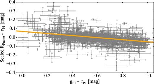
Colour term of the red arm of NTT-EMMI used with a Bessel R filter. The scaled difference of the measured R magnitudes and the PS1 rP1 magnitudes of the comparison stars from all used data sets are plotted against their PS1 (gP1 − rP1) colour indices. The orange line indicates the best linear fit to all points and its slope corresponds to the colour term. The colour term is used to correct the magnitude of the comparison stars before finding the zero-point of each frame taken with that instrument configuration.
Derived colour terms for all instruments used in this work.
| Instrument | Filter | ca | σcb | (gP1 − rP1) rangec |
|---|---|---|---|---|
| NTT-EMMI | R | −0.117 | 0.005 | 0.0–1.0 |
| NTT-EFOSC | R | −0.158 | 0.012 | 0.4–1.5d |
| NTT-EFOSC | r΄ | −0.194 | 0.005 | 0.0–1.5 |
| VLT-FORS2 | Re | −0.071 | 0.006 | 0.0–1.0 |
| WHT-PFIP | R | −0.100 | 0.008 | 0.0–1.0 |
| INT-WFC | r΄ | −0.007 | 0.002 | 0.0–1.5 |
aColour term c derived from comparison with PS1 star magnitudes in rP1 and gP1.
bUncertainty in the colour term.
cRange of the PS1 gP1 − rP1 colour indices of the used stars. Colour indices < 1 for Johnson-Cousins R filters and <1.5 for SDSS r filters.
dThis range was selected due to an insufficient number of stars with gP1 − rP1 < 0.4 in the observations used in this paper.
eESO R_SPECIAL+76 filter with effective wavelength 655 nm and FWHM 165.0 nm.
In order to use the colour term, we need to know the comet's colour index. The surface colours of JFCs are relatively well constrained with average colour indices (V − R) = 0.50 ± 0.03 and (B − V) = 0.87 ± 0.05 (Lamy et al. 2009). The (V − R) colour index can be converted to SDSS filter system: (g΄ − r΄) = 0.67 ± 0.06 using the relations in Jester et al. (2005) and to (gP1 − rP1) = 0.58 ± 0.06 in the PS1 system (Tonry et al. 2012). Since no further colour information was available for most comets, this colour index was used for the absolute calibration throughout the analysis.
The next step was to find the zero-point of the reference frame from the difference between the colour-corrected frame magnitudes and the corresponding PS1 rP1 magnitudes. With the colour term and the zero-point of the reference frame at hand, we converted the comet's magnitude to the PS1 system. Once the comet magnitude on the reference frame was converted to PS1 rP1 magnitudes, we shifted all the relative magnitudes to produce an absolutely calibrated light curve of the comet for each night.
3.4.4 Observing geometry correction
For most comets we have data from different epochs, which could be used to derive a phase function slope β independently. In all other cases, where the observations covered phase angle ranges smaller than 2°, we used β of 0.04 mag deg−1 to find the absolute magnitude of the nucleus Hr. For such single-run observations, we used the frame magnitude mr, rather than Hr, to derive the light curves.
3.4.5 Checking for activity
To determine whether the comets were active at the time of the observations, we compared the average comet PSF profile to that of a star. We first median-combined all sky-subtracted images for the night to produce a deep image of the background stars without cosmic rays and the moving comet. We then scaled this image and subtracted it from each comet frame in order to remove the background stars. Next, we centred each difference frame on the comet and combined all frames using a median filter, removing all cosmic rays. Finally, the measured comet profile on the combined frame was compared to the PSF of a bright star measured on the combined star field image.
In some cases described in detail below, the comet profile was noticeably different from that of the comparison stars (see Sections 4.2 and 4.3). This was interpreted as a strong indication of activity around the time of the observations. Nevertheless, we attempted to use these data sets to estimate the rotation rates and the properties of the nuclei. However, the derived results need to be interpreted with caution.
3.4.6 Period search
We used the Lomb–Scargle (LS) method (Lomb 1976; Scargle 1982) to detect periodicities in the brightness variation of the observed nuclei. LS is among the most widely used methods for finding periods in unevenly sampled time series. We ran the pythongatspy6LombScargleFast implementation of LS (VanderPlas & Ivezic 2015) to look for periods between 3 and 40 h. In the cases where the nightly brightness variations suggested slower rotation, we extended the range to cover larger periods. Since we sampled a large range of possible periods, we computed the periodogram with the option of LombScargleFast to automatically determine the period grid. This guaranteed that the longer periods are as well sampled as the shorter ones.
We assumed that the brightness variation of the comets is a result of their shape rather than surface albedo variations. As the light curves of elongated bodies have two minima and two maxima per rotation cycle, we focused our search on double-peaked light curves. Experience shows that LS periodograms preferentially fit single-peaked light curves. Therefore, we interpreted the derived peaks in the periodograms as half the rotation period of comets.
The LS periods were cross-checked using two other methods for detecting periods of unevenly spaced samples: phase dispersion minimization7 (PDM; Stellingwerf 1978) and string-length minimization (SLM; Dworetsky 1983). For all comets below, the three methods detected the same set of possible periods and showed general agreement. Therefore, for simplicity, we have chosen to show only the LS periodograms.
3.4.7 Nucleus size and shape and density estimates
The reported uncertainties on the radii are based only on the photometric uncertainty. They do not account for the uncertainties introduced by the albedo and the phase function slope. The albedos of JFCs are between 2 and 7 per cent (see Table 5), which is within a factor of 2 of the commonly assumed value of 4 per cent. Therefore, the radius estimate can vary with maximum |$\sqrt{2}$| from the reported value. Since we observed all comets in a narrow phase angle range (typically <10 deg), the influence of the phase function uncertainty is also small. In the worst case, if the phase function slope varies with up to 0.08 mag deg−1, the absolute magnitude of the comet will vary with 0.8 mag, and the estimated radius will be within a factor of 1.5 from the estimated value.
3.4.8 Monte Carlo method
Determining the uncertainty in the light-curve period is a challenging and often neglected task. In this work, this problem is often additionally complicated by the large time span between the different observations, which leads to aliases in the periodograms. Additionally, as is shown for the individual comets below, sometimes more than one period seems to characterize the variation well, and it is not possible to decide on the most likely spin rate. In such cases, providing an uncertainty in the determined period based just on the information on the periodogram (e.g. FWHM of the highest peak) can be misleading.
Moreover, it is not clear to what extent the detected periods are influenced by the intrinsic uncertainties of the comet magnitudes. Two main effects are at play when considering what might dominate the uncertainties of the available time series. First, the data from the different nights are linked using absolute calibration. In some cases the sky area under consideration has few stars, which increases the absolute calibration uncertainty. Secondly, when we combine observations from two different observing runs, the applied phase angle correction determines the relative difference between the comet magnitudes from the different epochs. This effect is hard to quantify, unless the influence of the different possible phase function correction parameters is explored.
In an attempt to account for these effects, we adopt a Monte Carlo (MC) method that allows us to retrieve better-validated values for the phase function coefficients and the rotation periods for the comets. The Monte Carlo method consists of the following steps:
Each magnitude from the time series of the comet is replaced by another randomly selected value. The new magnitude is selected from a normal distribution with mean equal to the original magnitude value and standard deviation equal to the uncertainty of the magnitude. The result is a clone i of the original time series, where the times and observing geometries are the same as the original time series, but the magnitudes were varied within the uncertainty space.
The clone magnitudes are used to find the best-fitting linear phase function coefficient βi.
The clone data set is corrected for the phase function by converting from m(1, 1, α) to m(1, 1, 0) using the derived βi.
The LS period search routine is run on the clone magnitudes m(1, 1, 0) to determine the best-fitting period Pi.
This procedure is repeated for i = 1, 2, …, 5000.
To determine the phase function coefficient, we plot the histogram of the determined βi and fit a Gaussian probability density function to it. In the final results, we report the best fit for the phase function coefficient to be the mean of the distribution, while its uncertainty is taken to be equal to the central 3σ range of the distribution.
To determine the most likely rotation period, we plot the histogram of the derived Pi and fit a Gaussian probability density function to it. As a final result we report the period of the comet as equal to the mean of the distribution, and an uncertainty equal to the central 3σ range of the fitted probability density function.
In all cases the distribution of the derived βi can be described well by a normal distribution. However, for some comets the Pi distributions are more irregular. In the cases when the distribution is irregular, we take the highest peak as the most likely period candidate, but we carefully explore the alternatives in the analysis.
4 TIME SERIES PHOTOMETRY RESULTS
4.1 14P/Wolf
The light curve of comet 14P/Wolf was first determined from two observing nights close to aphelion in 2004 by Snodgrass et al. (2005). Our team observed 14P as part of SEPPCoN once more in 2007 during the same aphelion passage. We analysed both data sets with our method for absolute photometric calibration and combined them in order to constrain better the comet's rotational period.
We used the procedure described in Section 3.4.5 to check whether 14P was active during the observations in 2004. The comet appears stellar in the co-added comet composite image and its surface brightness profile is indistinguishable from that of the comparison star (Fig. 2). This confirms the conclusion of Snodgrass et al. (2005) that 14P was not active during the observations in 2004.
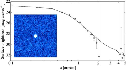
Surface brightness profile of 14P from the 2004 data set. The lower panel shows a 30 × 30 arcsec2 composite image of 14P made up of 29 × 220 s exposures taken on 2004 January 21. The frames are added in a method that removes cosmic rays, the background sky and fixed objects. The comet appears stellar and no signatures of activity can be recognized. The surface brightness of the comet is plotted as a function of radius ρ from the centre of the comet. The profile matches the scaled stellar PSF (solid line), indicating that the comet appears as a point source and is therefore considered to be inactive.
Fig. 3 shows the LS periodogram for the 2004 observations of 14P. The highest peak is at Pfit = 4.46 h, corresponding to a rotation period Prot = 8.93 h (Fig. 4). Using the Monte Carlo method without phase function correction, we determined that the best-fitting rotation period is Prot = 8.93 ± 0.04 h (Fig. 5).
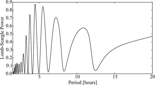
LS periodogram for 14P from the data set collected in 2004. The plot shows the LS power versus period. The highest peak occurs at 4.46 h, which corresponds to the most likely period Prot = 8.93 h.
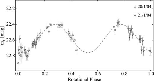
Rotational light curve of 14P with the data from 2004. The light curve is folded with the LS best period of 8.93 h.
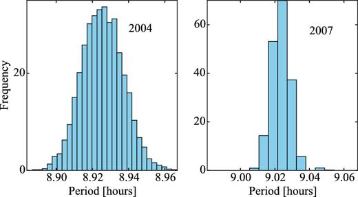
Results from the Monte Carlo simulations used to determine the rotation period of 14P from the data sets in 2004 (left) and 2007 (right). The resulting rotation periods for 2004 and 2007 are 8.93 ± 0.04 and 9.02 ± 0.04, respectively.
Using the same data set, Snodgrass et al. (2005) identified 7.53 ± 0.10 h as the most likely rotation period of 14P. That period corresponds to the third highest peak in our periodogram and results in an unusual asymmetric light curve. The difference in the periods likely originates from the different methods for night-to-night calibration adopted in the two works. While Snodgrass et al. (2011) used Landolt star calibration, here we applied our newly developed method for absolute calibration with PS1, which allows precise absolute calibration independent of the changing observing conditions during the night. Thus, by re-analysing the data from 2004 with our method, we improved the period determination of 14P.
The light curve of 14P in 2004 phased with Prot = 8.93 ± 0.04 h has a peak-to-peak brightness variation of Δmr = 0.36 ± 0.05 mag, which corresponds to axial ratio a/b ≥ 1.39 ± 0.06. From equation (6) we estimated a minimum nucleus density of 0.19 ± 0.04 g cm−3.
Next, we analysed the observations from 2007. The comet appears stellar on the composite images and its surface brightness profile does not deviate from that of the comparison star (Fig. 6). We can therefore assume that 14P was inactive at the time of the observations.
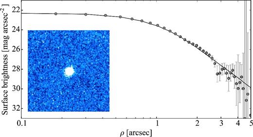
Same as Fig. 2, for 14P on 2007 May 18. The co-added composite image of 14P was made up of 18 × 70 s exposures. The stellar appearance on the composite image and the surface brightness profile of the comet suggest that 14P was inactive during the observations in 2007.
The highest peak of the LS periodogram for the 2007 observations is at Pfit = 4.51 h corresponding to a rotation period Prot = 9.02 h. (Fig. 7). We used the Monte Carlo approach without geometric corrections to determine a rotation rate Prot = 9.02 ± 0.04 h (right-hand panel on Fig. 5). The light curve phased with the identified period (Fig. 8) has a peak-to-peak variation Δmr = 0.39 ± 0.05 mag corresponding to a/b ≥ 1.43 ± 0.07 and DN ≥ 0.19 ± 0.04 g cm−3.
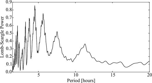
LS periodogram for 14P with the data set from 2007. The highest peak corresponds a period Prot = 9.02 h.
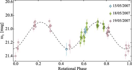
Rotational light curve of 14P with the data from 2007. The light curve is folded with period 9.02 h.
The periods from 2004 and 2007, around the same aphelion passage, are compatible within the uncertainties. Furthermore, the fact that the comet was inactive at both epochs suggests that 14P probably remained inactive around aphelion and a period change due to outgassing is unlikely to have occurred. Since we have no knowledge about the comet spin axis orientation, it is not possible to exclude the possibility that the viewing geometry changed between the two epochs. However, both individual light curves have the same peak-to-peak brightness variation (within the corresponding uncertainties), and therefore we can assume that the change in geometry did not influence the observed light curve. With these assumptions at hand, we proceeded to combine the two data sets in order to determine a phase function and a common rotation period.
We ran the Monte Carlo simulation on the combined data set and determined a phase function slope β = 0.060 ± 0.005 mag deg−1 and period Prot = 9.02 ± 0.01 h (Figs 9 and 10). The LS periodogram of the combined data sets (Fig. 11) has a pronounced peak at Pfit = 4.51 h which corresponds to the best period from the Monte Carlo simulation.
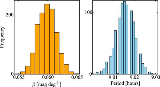
Monte Carlo simulation results for the phase function and the rotation period of 14P for the combined data set from 2004 and 2007. The determined linear phase function slope is β = 0.060 ± 0.005 (left) and the rotation period is Prot = 9.02 ± 0.01 h (right).
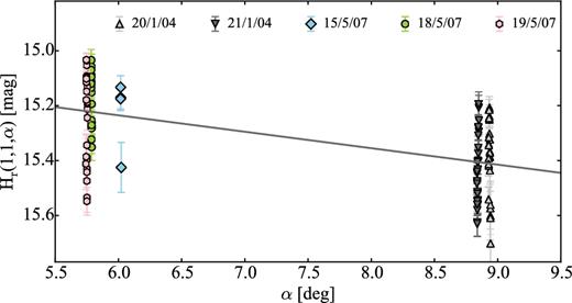
Phase function of comet 14P. The absolutely calibrated comet magnitudes corrected for heliocentric and geocentric distance are plotted versus phase angle α. The linear phase function with the best-fitting slope β = 0.060 ± 0.005 mag deg−1 is plotted as a solid line.
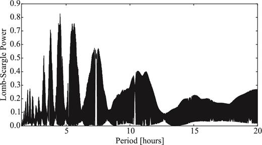
LS periodogram of 14P with the combined data sets from 2004 and 2007. The highest peak corresponds to the most likely period Prot = 9.02 h. The periodogram is very densely populated with peaks from the aliases which are present due to the large time span between the two observing runs.
The light curve phased with the best period Prot = 9.02 (Fig. 12) has a range ΔHr = 0.37 ± 0.05 mag corresponding to a/b ≥ 1.41 ± 0.06 and DN ≥ 0.19 ± 0.03 g cm−3. The mean absolute magnitude was Hr(1, 1, 0) = 14.87 ± 0.05 mag. Using equation (4) and the radius from Fernández et al. (2013), we estimated the comet's albedo to be Ar = 4.3 ± 0.6 per cent.
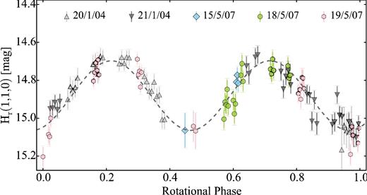
Rotational light curve of 14P/Wolf with the data from 2004 and 2007. The light curve is folded with period 9.02 h.
4.2 47P/Ashbrook–Jackson
The first attempt to determine the rotation rate of 47P was made by Snodgrass et al. (2006) using data from two observing nights in 2005. However, the resulting time series were not sufficient to choose between four possible periods: 11.2, 15.5, 21.6 and 44 h. Moreover, as discussed in Section 2.2.2, the attempts to determine the comet's phase function have also remained unconsolidated (Snodgrass et al. 2008b; Lamy et al. 2011).
In order to address these inconsistencies, we obtained new time series observations of the comet in 2015 April. The new data were taken at a different apparition than those from 2005, and could not be used to look for a common period without introducing further uncertainties. Nevertheless, the two data sets could still be combined for an attempt to derive the phase function of the nucleus.
Upon re-analysing the 2005 data set, we found that 47P was faintly active during the observing run. However, the inner surface brightness profile of the coma matched that of the comparison star well, suggesting that the activity was clearly weak (Fig. 13).
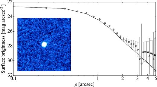
Same as Fig. 2, for 47P on 2005 March 6. The co-added composite image of 47P is made up of 27 × 85 s exposures. The surface brightness profile of the comet slightly deviates from the stellar one beyond 2 arcsec, which suggests that the comet was weakly active during the time of the observations.
We re-analysed the data from 2005 using our new absolute-photometry calibration method. The PS1 night-to-night calibration led to the identification of a smaller brightness variation and different possible periods than those in Snodgrass et al. (2006). The two strongest peaks of our LS periodogram were at Prot,1 = 10.8 and Prot,2 = 14.1 h (Fig. 14), and it is impossible to choose between them unambiguously (Fig. 15). The brightness variation of the resulting light curve was Δmr = 0.33 ± 0.06 mag suggesting axial ratio of a/b ≥ 1.36 ± 0.07.
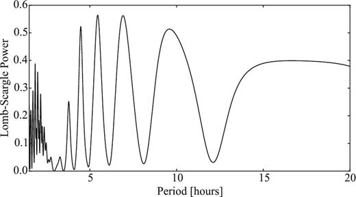
LS periodogram of 47P with the data from 2005. The two highest peaks correspond to Prot,1 = 10.8 h and Prot,2 = 14.1 h.
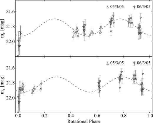
Rotational light curve of 47P with the data from 2005, folded with periods 10.8 h (top) and 14.1 h (bottom). It is impossible to select between these two periods.
When 47P was observed again in 2015, it appeared to be slightly active (Fig. 16). Nevertheless, the new time series showed sufficient brightness variation to enable a rotation period determination. The two highest peaks on the LS periodogram of the 2015 data set suggested Prot,1 = 15.6 h or Prot,2 = 23.7 h (Fig. 17). However, we consider that Prot,2 = 23.7 h is an alias due to the nightly sampling of the observations. Phasing the light curve of the comet with 23.7 h produced a non-realistic noisy light curve, and confirmed that this period does not correspond to the rotation rate of 47P.
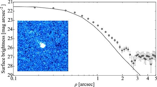
Same as Fig. 2, for 47P on 2015 April 24. The co-added composite image of 47P is made up of 26 × 80 s exposures. The comet appears to be slightly active with a tail detected to the north-east.
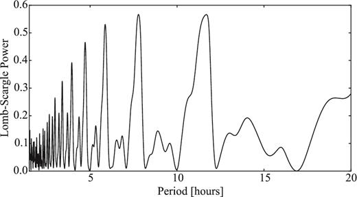
LS periodogram of 47P with the data from 2015. The two highest peaks correspond to Prot = 23.7 h and Prot = 15.6 h, although the period of 23.7 is most likely a 24-h alias.
We ran the Monte Carlo simulation for periods between 3 and 23 h (to avoid the 24-h alias) and determined Prot = 15.6 ± 0.1 h. The resulting plots of the MC simulation here and for most objects below are not shown since they are similar to Fig. 9, and do not provide additional information on the simulation outcomes. The brightness variation of the light curve (Fig. 18) was Δmr = 0.24 ± 0.06 mag, suggesting a/b ≥ 1.25 ± 0.07 and DN ≥ 0.06 ± 0.02 g cm−3.
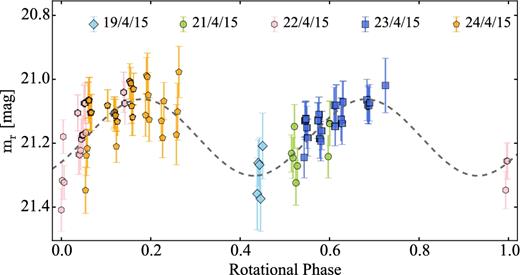
Rotational light curve of 47P with the data from 2015. The light curve is folded with the period of 15.6 h derived from the MC method.
Besides deriving the light curve of the comet, one of the main aims of the new observations from 2015 was to constrain the phase function of 47P. To address this, we first considered the previous brightness measurements from Licandro et al. (2000), Lamy et al. (2011) and Snodgrass et al. (2008b). Their magnitude measurements were converted to PS1 magnitudes using the colour indices of 47P (B − V) = 0.78 ± 0.08 and (V − R) = 0.40 ± 0.08 (Lamy et al. 2011), and the conversions from Tonry et al. (2012).
Additionally, we attempted to add an archival VLT data set from 2006 June when the comet was close to aphelion. However, these observations could not be used since the comet was clearly active on the frames (Fig. 19). Instead, these data complemented the data set from 2006 March (Snodgrass et al. 2008b), and confirmed that the comet had an outburst around aphelion.
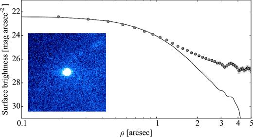
Same as Fig. 2, for 47P on 2006 June 1. The co-added composite image is made up of 4 × 300 s exposures. Due to the small number of frames, the composite image was made without subtraction of the average stellar background in order to avoid artefacts from the comet's slow position change. The comet appears active on the image, and its surface brightness profile deviates from the stellar PSF.
To derive the phase function coefficient β, we used the Monte Carlo approach considering only the long time series from 2005 and 2015. We did not include the other observations where the comet was active, or where the photometric calibration had been done using different methods. The Monte Carlo method resulted in a coefficient β = 0.096 ± 0.004 mag deg−1. The derived phase function appears to be in good agreement with all previous observations (Fig. 20), although it is unusually steep compared to the typical phase function for JFCs (see Table 5).
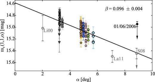
Phase function of comet 47P derived from the observing runs in 2005 and 2015. The symbols from 2005 and 2015 correspond to these used on Figs 15 and 18. The linear phase function slope β determined with the MC method is 0.096 ± 0.004 mag deg−1. Despite being unusually steep, the phase function is consistent with the previous observations of the comet from Licandro et al. (2000), Snodgrass et al. (2008b) and Lamy et al. (2011). However, since the comet was probably active in 2005 and 2015, the derived phase function slope is not conclusive.
Using that value for β to convert the observed magnitude, we calculated Hr(1, 1, 0) = 14.59 ± 0.06 mag. Using the radius from SEPPCoN and equation (4), we derived an albedo Ar = 5.0 ± 0.7 per cent.
We interpret these results with caution because of the slight activity detected on the stacked frames from 2005 and 2015, as well as the unusually steep phase function. If the coma contribution was large and/or the actual nucleus phase function slope was shallower, we would expect the absolute magnitude of 47P to be fainter. In that case, the comet must also have a smaller albedo (Ar ≤ 5.0 per cent).
Similarly, the derived period Prot = 15.6 ± 0.1 h must also be regarded as uncertain. The comet was found to be active at the time of the observations and therefore the nucleus signal was likely dampened by the present coma making the brightness variation more difficult to detect. Since the periods from both epochs were uncertain due to the limited sampling and the potential activity, we could not search for period changes occurring between 2005 and 2015.
4.3 93P/Lovas
93P/Lovas was observed with three different instruments during six nights in 2009 January as part of SEPPCoN. The observations were taken at heliocentric distance of 3.8 au when 93P was outbound. The composite images of the comet from each night contained traces of activity, and a tail to the west could clearly be resolved on the VLT frames (Fig. 21).
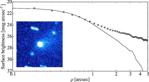
Same as Fig. 2, for the VLT observations of 93P on 2009 January 24. Due to the small number of frames, the composite image was made without subtraction of the average stellar background in order to avoid artefacts from the comet's slow position change. The co-added composite image is made up of 8 × 250 s exposures. A tail to the west can be clearly distinguished. The comet profile appears stellar close to the centre but deviates from that of the comparison star at larger radii.
Despite the weak activity, the brightness variation in the time series from each night suggested that the nucleus signal could still be detected. The LS periodogram of the combined data set can be seen in Fig. 22. The strongest peak at ∼24 h does not produce a typical light curve and corresponds to a 24-h alias. From the remaining peaks, those at Prot = 18.2 h and Prot = 13.2 h result in possible light curves (Fig. 23).
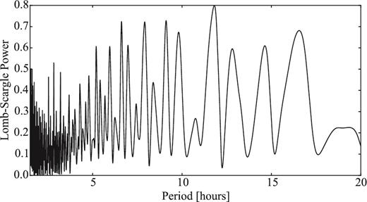
LS periodogram of 93P showing the LS power versus period. The highest peak corresponds to a 24-h alias. The next three peaks correspond to Prot = 18.2, 13.2 and 15.8 h.
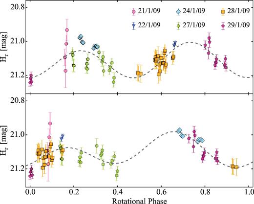
Rotational light curve of 93P folded with the two most likely periods 18.2 (top) and 13.2 h (bottom). The dashed line corresponds to second-order Fourier series that aim to reproduce an asymmetric double-peaked light curve. The light curve phased with 13.2 h shows less scatter, but the data are not sufficient to discriminate between the two periods.
We used the MC method to look for the best period between 3 and 23 h (to avoid the aliasing at 24 h). The simulation resulted in possible periods between 13.1 and 19.7 with the most frequently preferred period of 18.2 h (29 per cent of the iterations, Fig. 24). It is impossible to deduce the precise spin rate of 93P from these data, but the period can be constrained to the range |$P_{\mathrm{rot}}=\mathrm{18.2^{+1.5}_{-5}}$| h.
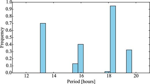
Monte Carlo simulation results for the rotation period of 93P. The most frequently preferred rotation period is 18.2 h, but the large range of possible periods does not allow us to uniquely determine the rotation rate of the comet.
The brightness variation of 93P is Δmr = 0.21 ± 0.05 mag and suggests an axial ratio a/b ≥ 1.21 ± 0.06. The mean magnitude of the comet is mr = 21.09 ± 0.05 mag which corresponds to Hr(1, 1, 0) = 15.17 ± 0.05 mag, for a typical phase function β = 0.04 mag deg−1. Using equation (4) and the SEPPCoN radius from Fernández et al. (2013), we estimate that the albedo of 93P is Ar = 4.2 ± 0.9 per cent.
Since the comet showed signatures of activity during the time of the observations, the brightness and albedo values we have derived need to be treated as upper limits. If the coma contribution of the frames is significant, the absolute magnitude of the nucleus must be larger, and therefore the resulting albedo must be smaller. In order to derive more certain estimates of the nucleus parameters, the comet needs to be observed at higher heliocentric distances where it is more likely to be inactive.
4.4 94P/Russell
In the analysis described here, we attempted to determine the rotation rate of 94P/Russell after combining three data sets from 2005, 2007 and 2009. The observations were taken before and after the same aphelion passage in 2007.
The data set from 2005 was previously used to determine a period of ∼33 h (Snodgrass et al. 2008b). We re-processed the data and used our method for absolute calibration to combine the observations from the four observing nights in 2005.
The surface brightness profile presented in Snodgrass et al. (2008b) suggested that the comet could have been weakly active at the time of the observations. We performed a careful background subtraction of the comet composite images for each night, and concluded that 94P appeared stellar on each night of the run (see Fig. 25).
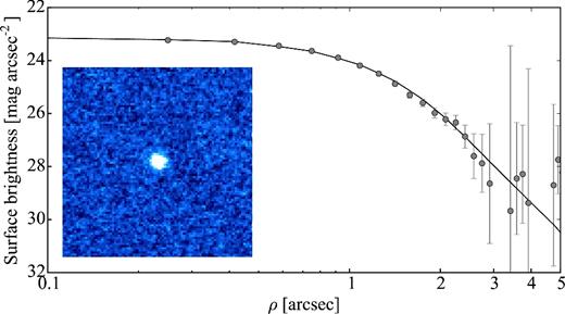
Same as Fig. 2, for the observations of 94P in 2005. The co-added composite image is made up of 15 × 75 s exposures taken on 2005 July 7.
The LS periodogram of the data taken in 2005 has two strong peaks corresponding to 20.43 and 14.31 h (Fig. 26). The light curves phased with these periods are plotted in Fig. 27. It is not possible to reject the second-best period based on the appearance of the light curve. However, in all iterations of the MC simulation the larger period was preferred and therefore the period was determined to be Prot = 20.43 ± 0.05 h.
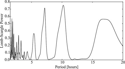
LS periodogram of 94P from the data set taken in 2005. The highest peaks correspond to the most likely periods Prot,1 = 20.43 h and Prot,2 = 14.31 h.
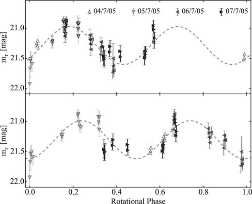
Rotational light curve of 94P from the data obtained in 2005. The light curve is folded with Prot,1 = 20.43 h (top) and Prot,2 = 14.31 h (bottom). We cannot choose between the two periods based on the appearance of the two light curves. However, Prot,1 = 20.43 h is preferred by the MC method, and is therefore considered as more likely.
The resulting light curve had a brightness variation Δmr = 0.7 ± 0.1 mag. This corresponds to an axial ratio a/b ≥ 1.9 ± 0.2 and density DN ≥ 0.05 ± 0.01 g cm−3.
The data taken during the SEPPCoN runs in 2007 and 2009 were also checked for the presence of activity (Figs 28 and 29). Due to the faintness of the comet, in both cases its surface brightness profiles levelled out within 5 arcsec from the nucleus. However, we can conclude that 94P was inactive in both epochs considering the good matches with the stellar PSF close to the centre, as well as the appearance of the composite images.
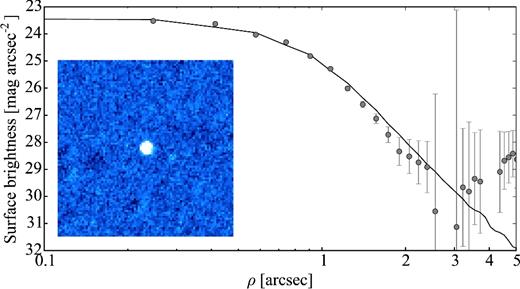
Same as Fig. 2, for the observations of 94P in 2007. The co-added composite image is made up of 8 × 400 s exposures taken on 2007 July 20.
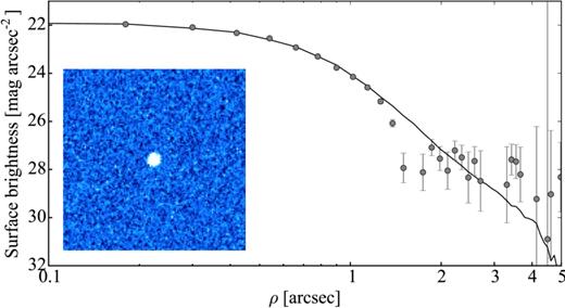
Same as Fig. 2, for the observations of 94P in 2009. The co-added composite image is made up of 8 × 100 s exposures taken on 2009 January 28.
Neither of the two data sets from 2007 and 2009 were sufficient to derive the rotation rate of 94P independently. We therefore only used them to estimate the nucleus magnitude and the minimum brightness variation at each epoch. We measured mr = 22.6 ± 0.2 and Δmr = 1.0 ± 0.2 mag for 2007, and mr = 21.30 ± 0.05 and Δmr = 0.80 ± 0.05 mag for 2009.
We combined all three data sets to determine the precise rotation rate of the comet. The analysis of the joined data sets was done under the following assumptions: (1) the comet was inactive during all observations and the measured magnitudes had no coma contributions; (2) the rotation period remained constant during the entire aphelion passage and (3) the changing viewing geometry between the different observations did not affect the light-curve shape significantly.
With these assumptions in mind, we used the MC method to derive a phase function with a slope β = 0.039 ± 0.002 mag deg−1 (Fig. 30). The LS periodogram of the combined data set on Fig. 31 peaks at Prot = 20.70 h. The period Prot = 20.70 h was also suggested by PDM and SLM. The other two peaks of the LS periodogram close to 38 and 40 h were also inspected but their light curves were significantly noisier.
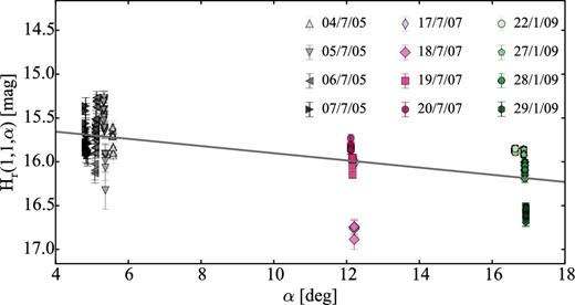
Phase function of comet 94P combining the data sets from 2005, 2007 and 2009. The linear phase function coefficient derived with the Monte Carlo method is β = 0.039 ± 0.002 mag deg−1.
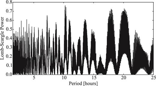
LS periodogram of 94P with the data sets from 2005, 2007 and 2009 combined. The highest peak corresponds to the most likely period Prot = 20.70 h.
The period of 20.70 h was preferred in 86 per cent of the MC iterations, which allows us to set the rotation rate of 94P to Prot = 20.70 ± 0.07 h. The corresponding light curve plotted in Fig. 32 shows a very good agreement between the separate data sets.
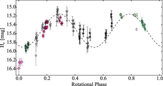
Rotational light curve of 94P with the combined data sets from 2005, 2007 and 2009. The symbols of each data set correspond to those used on Fig. 30. The light curve is folded with the best-fitting period Prot = 20.70 h. The fitted first-order Fourier series (dashed line) agree with all points except for the ones from 2007 July 18. These fainter points could be interpreted as signatures of an asymmetric light curve with one deep minimum, or alternatively as results from the changing viewing geometry between the three epochs.
The absolute magnitude of 94P from the combined data set was Hr(1, 1, 0) = 15.50 ± 0.09 mag. The albedo of 94P was determined with equation (4) to be Ar = 4.0 ± 0.6 per cent.
The only data sets that deviate from the first-order Fourier series in Fig. 32 are the ones from 2007 July. These points are fainter than the comet magnitude from the rest of the nights. There were no indications of problems with the images or the photometric calibration during these nights. We can conclude that the light curve must be asymmetric, with one of the minima being sharper and deeper than the other one. Such a light curve would have Δmr = 1.11 ± 0.09 mag which corresponds to a/b ≥ 2.8 ± 0.2 and density DN ≥ 0.07 ± 0.02 g cm−3.
Another effect that could produce the observed light curve is the change of viewing geometry. Comet 94P moved approximately 120° along its orbit between 2005 and 2009, which could be sufficient to produce a noticeable variation in the total surface area of the nucleus for an observer on Earth. Alternatively, the shift in brightness might be caused by weak activity in the 2005 and 2009 data when the comet was closer to the Sun. Such activity is not evident in the profiles on Figs 25, 28 and 29 but it is possible for some weak activity to be hidden within the seeing disc of distant comets (e.g. Snodgrass et al. 2016). With the limited data here, we cannot determine whether the deep minimum in the light curve is a feature of the nucleus or if it is caused by other effects.
4.5 110P/Hartley 3
Comet 110P/Hartley 3 was observed with VLT-FORS2 and NTT-EFOSC2 during eight nights between 2011 June and August. The aim of the observations was to sample the comet's phase function in the phase angle range between 1° and 10°. The method for precise absolute photometric calibration with PS1 allowed us to combine these data sets and to derive the comet's phase function as well as to study its rotational light curve.
We looked for signatures of activity on comet composite images for each individual night, and on Fig. 33 we have presented an example for the middle of the observing period. The comet did not show any indication of coma presence throughout the observing period, and we assume that the derived photometry from each night contains only signal from the nucleus.
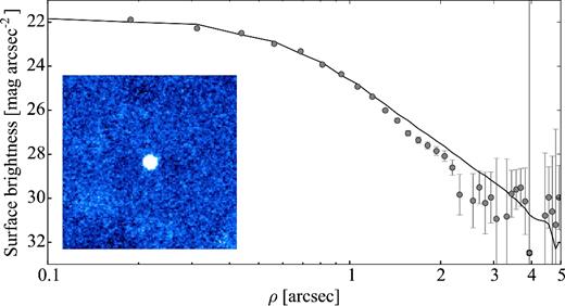
Same as Fig. 2, for 110P on 2012 July 15. The co-added composite image is made up of 18 × 70 s exposures. The comet appears inactive and its surface brightness profile follows that of the comparison star.
We used the MC method to derive a phase function for 110P. The determined phase function with linear slope β = 0.069 ± 0.002 mag deg−1 is in excellent agreement with all individual data sets (Fig. 34).
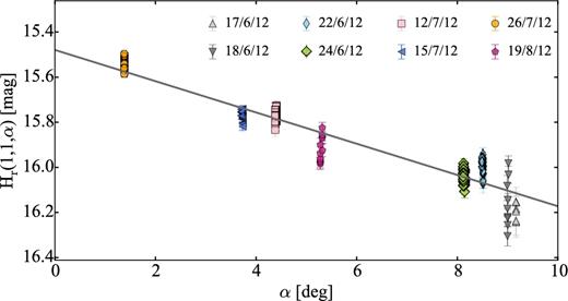
Phase function of comet 110P. The linear slope β derived with the Monte Carlo method is 0.069 ± 0.002 mag deg−1. The NTT-EFOSC2 points from 2012 June 17 and 18 were binned since the S/N of the individual points was low due to bad observing conditions.
All data sets were used to derive the comet's light curve under the same assumptions as those described earlier for 14P, 47P and 94P. The LS periodogram in Fig. 35 has three pronounced peaks at Prot,1 = 10.153 h, Prot,2 = 8.375 h and Prot,3 = 6.779 h. The MC method outlines Prot,1 = 10.153 ± 0.001 h (75 per cent of the iterations) and Prot,2 = 8.375 ± 0.001 h (17 per cent of the iterations) as most likely solutions (Fig. 36). Qualitatively, the light curve phased with Prot,1 = 10.153 ± 0.001 h presents less scatter of the points and agrees with the trends in the individual observing blocks better. Since Prot,1 is also preferred by the MC method, we report 10.153 ± 0.001 h as the most likely period of 110P.
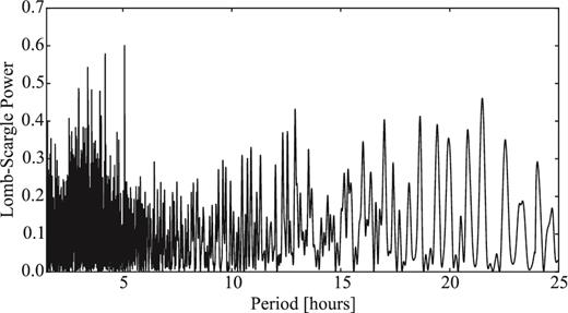
LS periodogram of 110P for the combined data set with all observations from 2012. The three highest peaks correspond to Prot,1 = 10.153 h, Prot,2 = 8.375 h and Prot,3 = 6.779 h.
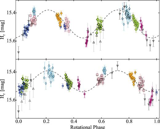
Rotational light curve of 110P with all of the data from 2012. The light curve is folded with the two most likely periods 10.153 (top) and 8.375 h (bottom) derived from the MC method. The light curve with Prot,1 = 10.153 h is preferred by the MC method (in 75 per cent of the iterations) and it is in better agreement with the brightness variation within the individual nights. The symbols are the same as in Fig. 34. The NTT-EFOSC2 points from 2012 June 17 and 18 were binned since the S/N of the individual points was low due to bad observing conditions.
The brightness variation of the resulting light curve is Δmr = 0.20 ± 0.03 which puts a lower limit on the comet axial ratio a/b ≥ 1.20 ± 0.03. Using Prot,1, we can estimate the nucleus density DN ≥ 0.13 ± 0.02 g cm−3. The mean absolute magnitude of the comet was Hr(1, 1, 0) = 15.47 ± 0.03 mag, which corresponds to a nucleus radius rN = 2.31 ± 0.03 km, assuming an albedo of 4 per cent.
Our results are in good agreement with those of (Lamy et al. 2011, see Section 2.2.5). This validates our results and confirms that it is possible to constrain both the phase function and the light curve of the comet from sparse observations spread over months. Although the two observations were taken at different apparitions and a small period change could have occurred during the active phase of the comet, due to the large uncertainty in the period from Lamy et al. (2011), we cannot search for period changes between the two epochs.
4.6 123P/West–Hartley
This SEPPCoN target was observed on three consecutive nights in 2007 July while it was at heliocentric distance of 5.6 au. A careful examination of the images indicated that despite the large heliocentric distance at the time of the observations, 123P was weakly active (Fig. 37).
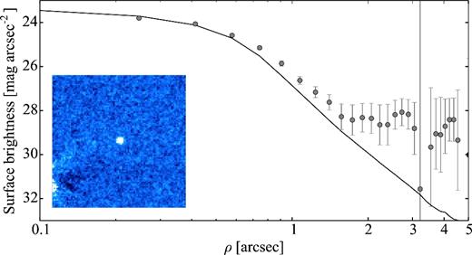
Same as Fig. 2, for 123P on 2007 July 18. The co-added composite image is made up of 23 × 110 s exposures. The comet appears stellar on the composite image; however, its surface brightness profile deviates from that of the comparison star, which indicates that the comet was weakly active during the time of the observations.
The observations from the individual nights clearly indicated a brightness variation of the nucleus. However, the LS periodogram of the data did not reveal any pronounced peaks with significant power (Fig. 38). The two highest peaks correspond to 3.7 and 10.3 h. Those two periods were also preferred by the MC simulation, which picked Prot = 3.70 ± 0.02 h in 66 per cent of the iterations and Prot = 10.27 ± 0.05 h (34 per cent).
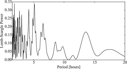
LS periodogram of 123P. The two highest peaks correspond to Prot,1 = 3.7 h and Prot,2 = 10.7.
The light curves resulting from these two periods are plotted in Fig. 39. Both periods appear to be in agreement with the data, and it is not possible to choose between them. Moreover, the data phased with other periods selected by the periodogram produce light curves with similar quality. Therefore, we conclude that the collected data are not sufficient to determine the spin rate of 123P.
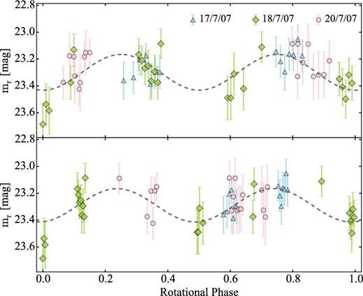
Rotational light curve of 123P with all of the data from 2007. The light curve is folded with the most likely periods 3.7 (top) and 10.7 h (bottom).
We estimated a brightness variation Δmr = 0.5 ± 0.1 mag which corresponds to an axial ratio a/b ≥ 1.6 ± 0.1. The mean measured magnitude of 123P was mr = 23.3 ± 0.1 mag which converts to Hr(1, 1, 0) = 15.7 ± 0.1 mag if a phase function with β = 0.04 mag deg−1 is used. Our absolute magnitude and the radius measured by Fernández et al. (2013) convert to an albedo Ar = 3.6 ± 0.8 per cent (equation 4). It is however important to note that the surface brightness profile of 123P indicated a weak activity, which implies that the absolute magnitude Hr(1, 1, 0) of the nucleus could be fainter and the determined albedo must be treated as an upper limit.
4.7 137P/Shoemaker–Levy 2
Comet 137P was observed during one night in 2005 and two nights in 2007 as part of SEPPCoN. It appeared inactive during both observing epochs (Figs 40 and 41).
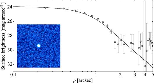
Same as Fig. 2 for 137P on 2005 March 6. The co-added composite image is made up of 23 × 110 s exposures. The comet appears inactive and its surface brightness profile follows that of the comparison star close to the centre before it levels out at the background noise level.
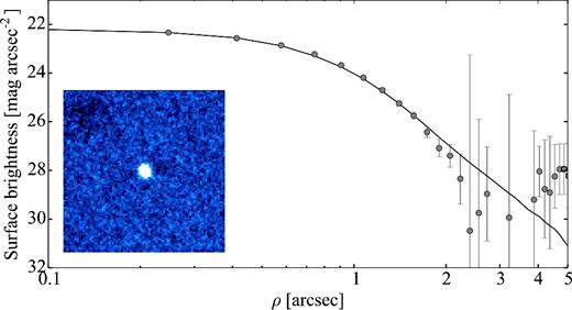
Same as Fig. 2 for 137P on 2007 July 13. The co-added composite image is made up of 20 × 75 s exposures. The comet appears inactive and its surface brightness profile matches that of the comparison star.
We applied the MC method on the combined data set from all three nights to determine the comet's phase function (Fig. 42). The derived phase function slope was β = 0.035 ± 0.004 mag deg−1.
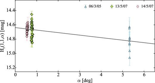
Phase function of comet 137P. The linear phase function coefficient derived from the Monte Carlo simulations is β = 0.035 ± 0.004 mag deg−1.
Next, we attempted to determine the light-curve period from the data taken in 2005. The highest peak of the periodogram in Fig. 43 corresponds to a rotation period of 7.7 h. However, all peaks on the periodogram have low powers which are not sufficient to determine the rotation rate of 137P.

LS periodogram of 137P from the 2007 data set. The highest peak corresponds to a period of Prot = 7.7 h.
The light curve phased with a period of 7.7 h is plotted in Fig. 44. Its brightness variation is Δmr = 0.18 ± 0.05 mag, which converts to a/b ≥ 1.18 ± 0.05. The uncertainties of the individual points are large in comparison with the detected brightness variation. Therefore, it is not possible to derive a precise rotation rate for the comet from this data set. We attempted to improve the period determination by combining all data from 2005 and 2007. However, the photometry from 2007 has even larger photometric uncertainties and does not lead to improvement of the period estimation.
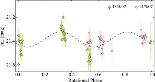
Rotational light curve of 137P with all of the data from 2007 folded with one of the possible periods, 7.7 h. The uncertainty of the points is large in comparison to the brightness variation of the comet, which obstructs the period determination.
The absolute magnitude of 137P is Hr(1, 1, 0) = 14.63 ± 0.05 mag. Using equation (4) and the SEPPCoN radius from Fernández et al. (2013), we estimated the albedo Ar = 2.8 ± 0.5 per cent.
4.8 149P/Mueller 4
Comet 149P was observed using NTT, WHT and VLT during seven nights at the end of 2009 January. The surface brightness profiles of the comet for each night indicated that it was not active at the time of the observations (see Fig. 45).
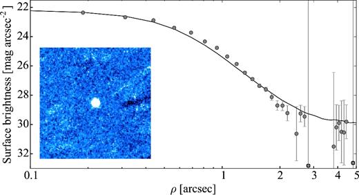
Same as Fig. 2 for 149P on 2009 January 23. The co-added composite image is made up of 15 × 80 s exposures. The comet appears inactive and its surface brightness profile matches that of the comparison star.
The phase angle of 149P changed between 8|$_{.}^{\circ}$|5 and 10° between the first and the last observing night. We used the MC method to constrain the phase function slope of the comet as β = 0.03 ± 0.02 mag deg−1 (Fig. 46).
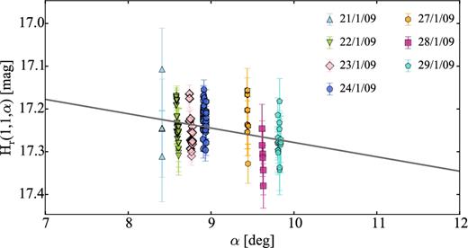
Phase function of comet 149P. The linear phase function coefficient derived from the Monte Carlo simulations is β = 0.03 ± 0.02 mag deg−1.
The periodogram of the time series corrected for geometric effects peaks at Prot = 11.9 h (Fig. 47). The period of 11.9 ± 0.1 is preferred by the MC simulation in 84 per cent of the iterations. However, the power of the peaks on the periodogram is too small and we cannot select the best period unambiguously. A rotation period near 12 h would make this measurement for 149P difficult, and a clear determination of such a period using an Earth-based facility would require a longer photometric time sequence.
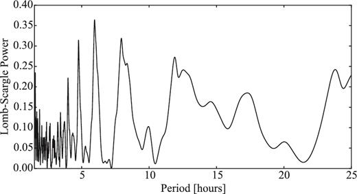
LS periodogram of the combined data sets for 149P showing the LS power versus period. The highest peak corresponds to the most likely period Prot = 11.88 h. Since all peaks have low power, the spin period of the comet cannot be determined unambiguously.
Fig. 48 shows the light curve of 149P with the best fit from the MC method. The photometric uncertainty of the individual points is large with respect to the total brightness variation of the light curve, which confirms that the derived light curve is uncertain.
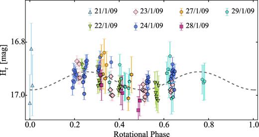
Rotational light curve of 149P with all of the data from 2009. The points from WHT and NTT were binned The light curve is folded with the most likely period of 11.88 h.
The brightness variation of the comet is Δmr = 0.11 ± 0.04 mag which converts to a/b ≥ 1.11 ± 0.04. The observed mean magnitude of 149P was mr = 22.14 ± 0.04 mag which corresponds to Hr(1, 1, 0) = 16.93 ± 0.04 if the derived phase function with β = 0.03 ± 0.02 mag deg−1 is used. Using equation (4), we can calculate that the albedo of 149P is Ar = 2.8 ± 0.4 per cent.
4.9 162P/Siding Spring
Comet 162P was observed in 2007 around its aphelion, and again in 2012 close to its next aphelion passage. The first set of observations aimed to determine the comet's light curve, while the second data set focused on its phase function.
The comet had a stellar profile and appeared to be inactive in 2007 (Fig. 49). The LS periodogram of the data from the three observing nights in 2007 is shown in Fig. 50. The most pronounced peak in the periodogram corresponds to Prot = 32.6 h, and the light curve phased with that period can be seen in Fig. 51. Using the MC method without phase function correction, we determined the rotation period of the comet to be Prot = 32.6 ± 1 h. This period is in good agreement with the value of ∼33 h determined by the team of La Cañada observatory (see Section 2.2.9).
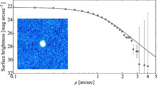
Same as Fig. 2, for 162P on 2007 May 18. The co-added composite image is made up of 10 × 110 s exposures. The comet appears inactive and its surface brightness profile agrees with that of the comparison star.
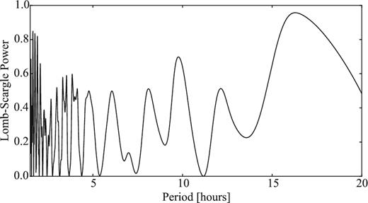
LS periodogram of the 2007 data set for 162P showing the LS power versus period. The highest peak corresponds to the most likely period Prot = 32.6 h.
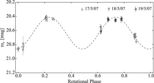
Rotational light curve of 162P with the data from 2007. The light curve is folded with period 32.6 h.
From the observations in 2007, we measured the mean magnitude of 162P to be mr = 20.63 ± 0.05 mag. The brightness variation of the comet was Δmr = 0.45 ± 0.05 mag, which corresponds to a/b ≥ 1.51 ± 0.07.
Comet 162P was also inactive during all observations in 2012, which is demonstrated by the surface brightness plot in Fig. 52. Since the observations were taken at a large phase angle range (4°–12°), we could only combine the data after deriving the comet's phase function. The MC method determined a phase function coefficient β = 0.039 ± 0.002 mag deg−1.
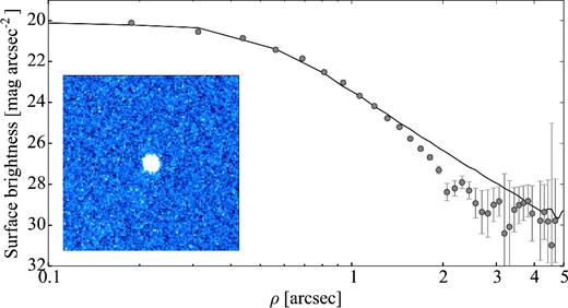
Same as Fig. 2, for 162P on 2012 April 23. The co-added composite image is made up of 5 × 60 s exposures. The comet appears inactive and its surface brightness profile generally agrees with that of the comparison star. The narrower profile of the comet is most likely an artefact of the position uncertainty of the comet on the frames.
The LS periodogram of the combined data set from 2012 suggested multiple possible rotation periods for 162P (Fig. 53). The MC method preferred Prot,1 = 33.237 ± 0.008 h in 62 per cent of the iterations and Prot,2 = 32.852 ± 0.003 h in 35 per cent of the iterations. The light curves in Fig. 54 confirm that due to the limited sampling of the light curve, it is impossible to choose between these two possibilities, although it is worth noting that the points from 2012 May 24 agree better with Prot,2 = 32.852.
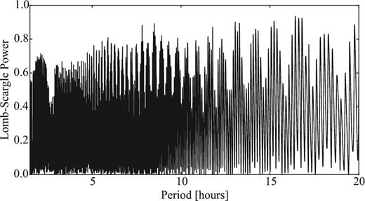
LS periodogram of the 2012 data set for 162P showing the LS power versus period. There are a number of possible periods as well as secondary peaks caused by aliasing. The highest peaks correspond to rotation periods of 32.852 and 33.237 h.
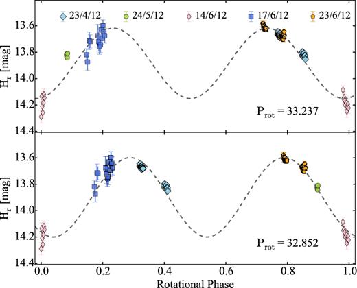
Rotational light curve of 162P with the data from 2012. The light curve is folded with Prot,1 = 33.237 h (top) and Prot,2 = 32.852 h (bottom). It is not possible to choose between the two periods from the data set collected in 2012.
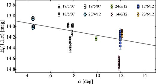
Phase function of comet 162P. The linear phase function slope derived from the Monte Carlo simulations is β = 0.038 ± 0.002 mag deg−1.
The brightness variation in the 2012 observations was Δmr = 0.59 ± 0.04 mag, which corresponds to a/b ≥ 1.72 ± 0.06. The absolute magnitude of 162P from the 2012 data set was Hr(1, 1, 0) = 13.91 ± 0.04 mag. If we use equation (4), we can estimate the albedo of 162P to be Ar = 1.8 ± 0.3 per cent. This result makes comet 162P the JFC with the lowest known albedo (see Section 5.4).
As a final step in the analysis of the data for 162P, we combined the two data sets from 2007 and 2012 in order to attempt constraining the comet's light curve and phase function better. It is possible that the period of 162P slightly changed between 2007 and 2012 while the comet was active close to perihelion. Besides, it is not excluded that since the two observations were done at different geometries, the resulting light curves can appear different. Nevertheless, it is worth attempting to combine the two data sets as the increased number of observations can provide a better understanding of the nucleus’ properties.
With these caveats in mind, we proceeded to analyse the combined data from 2007 and 2012. The MC method suggested a phase function with a slope β = 0.038 ± 0.002 mag deg−1 and a light curve with period Prot = 32.853 ± 0.002 h. This period corresponds to the highest peak of the LS periodogram in Fig. 56 .
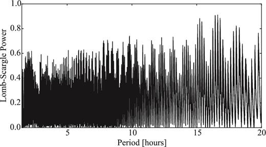
LS periodogram of the combined data sets of 162P from 2007 and 2012 showing the LS power versus period. The highest peak corresponds to Prot = 32.853 h.

Rotational light curve of 162P with the data from 2007 and 2012. The light curve is folded with the most likely period of 32.853 h.
The derived parameters from the combined data set are very close to those of the 2012 data set alone (See Table 4). However since they were derived using data from two different apparitions, we consider the values from just the 2012 data set to be less uncertain.
Derived physical parameters for all observed comets.
| Comet | Epoch | mra | Hr(1, 1, 0)a | Prot (h)b | β (mag deg−1)c | rN (km)d | Ar ( per cent)e | Δmr | a/b | DN (g cm−3) |
|---|---|---|---|---|---|---|---|---|---|---|
| 14P | 2004 | 22.58 ± 0.05 | – | 8.93 ± 0.04 | – | – | – | 0.36 ± 0.05 | 1.39 ± 0.06 | 0.19 ± 0.04 |
| 2007 | 21.06 ± 0.05 | – | 9.02 ± 0.04 | – | – | – | 0.39 ± 0.05 | 1.43 ± 0.07 | 0.19 ± 0.04 | |
| Combined | – | 14.87 ± 0.05 | 9.02 ± 0.01 | 0.060 ± 0.005 | – | 4.3 ± 0.6 | 0.37 ± 0.05 | 1.41 ± 0.06 | 0.19 ± 0.03 | |
| 47P | 2005f | 21.83 ± 0.06 | – | 10.8/14.1 | – | – | – | 0.33 ± 0.06 | 1.36 ± 0.07 | – |
| 2006f | 21.55 ± 0.04 | – | – | – | – | – | – | – | – | |
| 2015f | 21.11 ± 0.06 | 14.58 ± 0.06g | 15.6 ± 0.1 | – | – | – | 0.24 ± 0.06 | 1.25 ± 0.07 | 0.06 ± 0.02 | |
| 2005 + 2015h | – | 14.59 ± 0.06 | – | 0.096 ± 0.004 | – | 5.0 ± 0.7i | – | – | – | |
| 93P | 2009f | 21.09 ± 0.05 | 15.17 ± 0.05j | |$\mathrm{18.2^{+1.5}_{-15}}$| | – | – | 4.2 ± 0.9i | 0.21 ± 0.05 | 1.21 ± 0.06 | – |
| 94P | 2005 | 21.3 ± 0.1 | – | 20.43 ± 0.05 | – | – | – | 0.7 ± 0.1 | 1.9 ± 0.2 | 0.05 ± 0.01 |
| 2007 | 22.6 ± 0.2 | – | – | – | – | – | 1 ± 0.2 | 2.5 ± 0.5 | – | |
| 2009 | 21.30 ± 0.05 | – | – | – | – | – | 0.80 ± 0.05 | 2.09 ± 0.10 | – | |
| Combined | – | 15.50 ± 0.09 | 20.70 ± 0.07 | 0.039 ± 0.002 | – | 4.0 ± 0.6 | 1.11 ± 0.09 | 2.8 ± 0.2 | 0.07 ± 0.02 | |
| 110P | 2012 | – | 15.47 ± 0.03 | 10.153 ± 0.001 | 0.069 ± 0.002 | 2.31 ± 0.03 | – | 0.20 ± 0.03 | 1.20 ± 0.03 | 0.13 ± 0.02 |
| 123P | 2007f | 23.3 ± 0.1 | 15.7 ± 0.1j | – | – | – | 3.6 ± 0.8i | 0.5 ± 0.1 | 1.6 ± 0.1 | – |
| 137P | 2007 | 21.39 ± 0.05 | – | – | – | – | – | 0.18 ± 0.05 | 1.18 ± 0.05 | – |
| 2005 + 2007 | – | 14.63 ± 0.05 | – | 0.035 ± 0.004 | – | 2.8 ± 0.5 | – | – | – | |
| 149P | 2009 | 22.14 ± 0.04 | 16.93 ± 0.04 | – | 0.03 ± 0.02 | – | 2.8 ± 0.4 | 0.11 ± 0.04 | 1.11 ± 0.04 | – |
| 162P | 2007 | 20.63 ± 0.05 | – | 32.6 ± 1 | – | – | – | 0.45 ± 0.05 | 1.51 ± 0.07 | – |
| 2012 | – | 13.91 ± 0.04 | 33.237/32.852 | 0.039 ± 0.002 | – | 1.8 ± 0.3 | 0.59 ± 0.04 | 1.72 ± 0.06 | 0.017 ± 0.003 | |
| Combinedh | – | 13.90 ± 0.05 | 32.853 ± 0.002 | 0.038 ± 0.002 | – | 1.8 ± 0.3 | 0.62 ± 0.05 | 1.77 ± 0.08 | 0.018 ± 0.003 |
aMagnitudes in PS1 system.
bThe synodic rotation periods and their uncertainties were derived from the mean and standard deviation from the MC method (see Section 3.4.8).
cThe linear phase function coefficients and their uncertainties were derived from the mean and standard deviation from the MC method (see Section 3.4.8).
dCalculated from Hr(1, 1, 0) assuming an albedo A = 4 per cent.
eCalculated using equation (4) from Hr(1, 1, 0) and the effective radius Reff from (Fernández et al. 2013, see Table 1).
fThe comet was weakly active. The results do not include corrections for the presence of a near-nucleus coma.
gThe β value for the Hr(1, 1, 0) was taken from the phase function fit of the combined 2005 and 2015 data sets.
hThe data are from different apparitions.
iThe comet was weakly active at the time of the observation. The albedo estimates are therefore upper limits.
jCalculated for β = 0.04 mag deg−1.
5 DISCUSSION
In Table 1, we summarized the physical characteristics of all JFCs with known rotation rates. With the newly analysed light curves in Section 4, we have added six additional light curves, seven phase functions and eight albedo estimates. Here, we compare our newly obtained results with the overall JFC characteristics and use the expanded sample to draw conclusions about the collective population properties.
5.1 Spin rate distribution
The distribution of the rotation rates of comets can be used to study their collisional history. Fig. 58 shows a histogram of all known spin rates of JFCs. We have plotted the rotation frequency f = 1/Prot which was normalized using the geometric mean 〈f〉 of the whole sample. Similar plots for asteroids have shown that the distribution of asteroid spin rates is Maxwellian which has suggested that asteroids are a collisionally evolved population (Harris 1996; Pravec, Harris & Michalowski 2002).
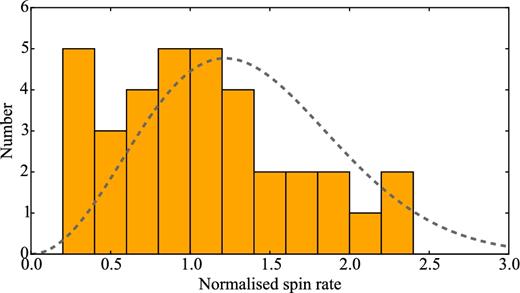
Histogram of the normalized rotation rates of 37 JFCs. The normalized spin rate is calculated as f/〈f〉 where f = 1/Prot and 〈f〉 is the geometric mean of f. The dashed line corresponds to the best-fitting Maxwellian distribution.
The best-fitting Maxwell distribution in Fig. 58 does not show good agreement with the measured spin rates. We performed Kolmogorov–Smirnov tests comparing the normalized frequency distribution in Fig. 58 to Maxwell distribution and flat distribution with the same mean and standard deviation. The resulting D statistics were 0.20 (p = 0.09) and 0.13 (p = 0.44) for the uniform and Maxwell distributions, respectively. We cannot reject the null hypothesis in either of the cases, and therefore both distributions can possibly describe the data.
The cumulative size distribution of JFCs was found to be very close to the one expected for a collisionally relaxed population of strengthless bodies (Lamy et al. 2004; Snodgrass et al. 2011; Fernández et al. 2013, and references therein). However, this result has a large uncertainty and cannot be used as a proof that JFCs originate from disrupted larger bodies (e.g KBOs). In turn, it suggests that due to the continuous mass-loss of JFCs, their size distribution can be shaped by a complex combination of collisional processes in the past and activity in the present epoch (Snodgrass et al. 2011).
Similarly, our results for the spin distribution of comets suggest that their rotation can be determined by the ongoing activity. The mass lost through activity jets is able to exert a torque on the nucleus, which in turn changes the spin rate of the comet on orbital time-scales (e.g. Samarasinha et al. 2004). This mechanism can be responsible for reshaping the original distribution of the spin rates, and could explain the current spin rate distribution of JFC. However, it is important to know that Fig. 58 includes data from just 37 comets, many of which have light-curve periods with large uncertainties. This highlights the need to increase the sample of JFCs with known rotational properties in order to enable the understanding of the population history.
It is worth noting that evidence from Rosetta, such as the low density/high porosity, and presence of hypervolatiles like O2 and N2, suggests that 67P is not a collisional fragment (see Davidsson et al. 2016, and references therein). The apparent coincidence of sizes and spin rates of JFC nuclei being consistent with collisional evolution, while in situ measurements of their bulk properties suggest otherwise, is surprising. This may instead support the hypothesis by Jutzi et al. (2017) that JFCs have undergone significant collisional evolution, but the distributions presented here do not yet allow a definitive conclusion.
5.2 Shapes
Fig. 59 shows the distribution of the axial ratios of all comets. Most a/b values are smaller than a/b = 2 and the median of the distribution is at a/b = 1.5. However, all comets with shape models obtained from in situ observations (9P, 19P, 67P, 81P, 103P) have significantly higher axial ratios (see Table 1). For all other objects the axial ratio is a lower limit since it was calculated from the light-curve brightness variation. It is therefore possible that the typical elongation of JFCs is higher than the one we estimated from the current distribution, suggesting that bilobate shapes (like those seen by spacecraft at 67P and 103P) may be common, in agreement with recent formation models (Davidsson et al. 2016).
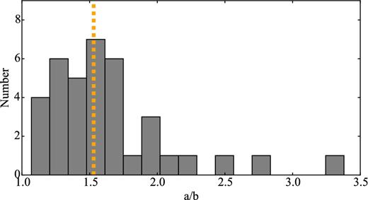
Distribution of the axial ratios a/b of JFCs. The vertical line corresponds to the median value of a/b = 1.5. For all comets (except 9P, 19P, 67P, 81P, 103P), the given axial ratio is obtained from ground- and space-based telescopes and is therefore just a lower limit of the elongation.
5.3 Bulk densities and stability against rotational splitting
We attempted to use the expanded sample of JFCs with estimated rotation rates and elongations to constrain the comet density and tensile strength. As we discussed in Section 3.4.7, it is commonly assumed that comets have negligible tensile strengths. Under this assumption, it is possible to set a lower limit on the density necessary to keep JFCs stable against rotational instabilities (equation 6; Pravec et al. 2002).
In Fig. 60, we plot the rotation versus projected axial ratio for all comets in the expanded sample. Using a similar plot, Lowry & Weissman (2003) discovered that comets do not require densities higher than approximately 0.6 g cm−3 in order to be stable against rotational instabilities. Here, we confirm this result for all objects except for 322P, 73P-C and 147P.
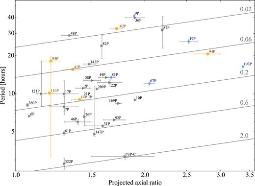
Rotation period against projected axial ratio for JFC nuclei. The grey triangles denote comets with parameters determined from light curve or radar measurements. The orange circles are the comets from this work. For these points, the axial ratio is a lower limit and the uncertainties are plotted when they were stated by the authors. The blue diamonds correspond to comets visited by spacecraft with precise shape models. The diagonal lines indicate the minimum density (denoted in g cm−3 to the right), which a strengthless body of the given axial ratio and spin period requires to remain intact. Apart from the unusual cases of 323P and 73P, which are discussed in the text, no comet requires a density greater than ∼0.6 g cm−3 to remain stable against rotational splitting.
As we discussed in Section 2.1.17, according to Knight et al. (2016) it is not clear whether 322P has asteroidal or cometary origin. Therefore, the fact that it requires higher density can be interpreted as evidence in favour of the hypothesis that it is an asteroid. Comet 147P lies very close to the limit of 0.6 g cm−3 and has a large period uncertainty. Therefore, we do not consider it as an outlier. Additionally, 147P belongs to the class of quasi-Hilda comets and might have asteroidal origin (Ohtsuka et al. 2008). Comet 73P-C on the other hand clearly has a JFC origin and therefore should be similar to the other objects in our sample. However, since it seems to be continuously disintegrating (see Section 2.1.7), it cannot be used to study the stability criterion. It is also possible that the breakup of the comet exposed the innermost part of the pre-breakup nucleus which could have a larger tensile strength (see Gundlach, Blum & Blum 2016, and references therein)
If we exclude these three comets, our expanded sample confirms the density limit of 0.6 g cm−3 discovered by Lowry & Weissman (2003). By analogy with the clear cut-off in rotation rates of asteroids at 2.2 g cm−3 (Pravec et al. 2002), we interpret the cut-off for comets as an indication that 0.6 g cm−3 is a typical density for JFCs. This agrees with the density estimates from recent spacecraft measurements (Richardson et al. 2007; Jorda et al. 2016).
Further insights into the material properties of JFCs can be determined from comparing their rotation rates and sizes. In previous studies, Davidsson (1999, 2001) and Toth & Lisse (2006) already explored the location of comets and other primitive minor bodies in the radius-rotation period plane. In Fig. 61, we plot the distribution of rotation rates with radius for all comets. A key feature of the distribution of comets in the plot is that the domain in the lower right corner is not populated.
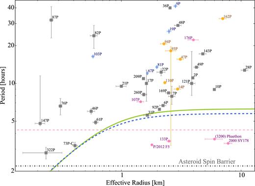
Rotation period against effective radius of the JFC nuclei. The blue diamonds are comets visited by spacecraft; the grey squares are comets observed from ground and the orange circles are the comets added in this work. For comparison, we plotted active asteroids with known rotation rates (pink pentagons). The lower horizontal dotted line corresponds to the asteroid spin barrier (Harris 1996; Pravec et al. 2002). The upper dashed pink line shows the minimum possible rotation rate for strengthless spherical bodies with density ρ = 0.6 g cm−3. The curves are derived from the model for prolate ellipsoids stable against rotational instability by Davidsson (2001). The solid green line is the model for density ρ = 532 kg m−3, axial ratio a/b = 2 and tensile strength T = 15 Pa, which corresponds to the parameters measured for 67P from Rosetta (Groussin et al. 2015; Jorda et al. 2016). The dashed blue curve is for the same density but a/b = 1.6 (the value for 31P) and T = 10 Pa. By varying the model parameters, we can conclude that for typical densities and axial ratios (a/b ≤ 2.0), none of the observed comets requires a tensile strength larger than 25 Pa to remain stable against rotational splitting.
In order to interpret this observation, we employ the recent results from the Rosetta mission. The in situ measurements of comet 67P provide precise estimates of the nucleus bulk parameters. It has density of 0.532 ± 0.007 g cm−3 (Jorda et al. 2016), axial ratio a/b = 2.05 ± 0.06 (calculated from the axis estimates in Jorda et al. 2016) and tensile strength of 3–15 Pa with an upper limit of 150 Pa (Groussin et al. 2015). If we assume that 67P is a representative example for JFCs, we can use these values to study the properties of the whole population.
In Fig. 61, we have plotted the asteroid spin barrier (Pravec et al. 2002) that corresponds to the minimum rotation period of a strengthless body with density ∼3 g cm−3. For a comparison, we have also plotted the rotation limit for a spherical object with density of 0.6 g cm−3. The position of the limit for comets will change for different elongations and densities since less dense and more elongated objects are easier to disrupt.
So far in the analysis, we have treated comets as strengthless; however, the measurements of the tensile strength of 67P allows us to explore more complicated models that take the material strength of comets into account. We have used the analytical models developed by Davidsson (1999, 2001) to determine the maximum rotation rate of prolate ellipsoids that are stable against rotational instabilities using the density, axial ratio and tensile strength of 67P (Fig. 61, solid green curve). This curve agrees very well with the observed data and puts 73P-C right at the limit of stability, which agrees with its frequent fragmentation events. Although comet 31P lies below the stability line, its projected axial ratio is lower than that of 67P.
We have therefore investigated the stability limit for objects with density of 0.5 g cm−3 and a typical axial ratio of a/b = 1.6 (equal to the elongation of 31P). We determine that under these assumptions none of the comets requires tensile strength higher than ∼10 Pa to remain stable against rotational instabilities (Fig. 61, dashed blue curve). We varied the axial ratio parameter of the model for ratios a/b ≤ 2.0 and concluded that none of the observed comets requires a tensile strength larger than 25 Pa to remain stable against rotational splitting. This confirms the low-tensile strength estimates of 67P by Groussin et al. (2015) and of Shoemaker–Levy 9 (Asphaug & Benz 1996).
An interesting test of this model would come from future observations of the rotation rate of 31P. The comet's period was previously very well determined by Luu & Jewitt (1992). If new observations of its light curve show that the nucleus is spinning up, this comet would be a strong candidate for future rotational splitting.
Despite the small number of nuclei with radii larger than 3 km in the sample, it is noticeable that all of them lie far above the stability limit. The simplest explanation for this effect could be deduced from the understanding of activity-induced rotational changes. According to the relations derived in Samarasinha & Mueller (2013), the rotation changes induced by outgassing are proportional to the square of the rotation period and inversely proportional to the square of the radius. In this scenario, if a large nucleus is spinning up due to reaction torques, the faster it gets, the less it can spin-up with every orbit. Therefore, it is very hard to spin-up the large nuclei that already rotate with relatively short periods.
At this stage, we cannot evaluate this hypothesis further since spin changes are poorly investigated and to this date only five comets have confirmed period changes (see Samarasinha & Mueller 2013, and references therein). To improve the understanding of the rotation of large comets, we need to measure the rotation rates of more large nuclei and to increase the number of comets with period determinations at multiple apparitions.
Finally, in Fig. 61, we have also plotted all active asteroids with known periods and radii (Jewitt et al. 2015). Most of them lie in the lower right domain of the plot where no JFCs can be found. However, it is particularly interesting to note that 107P fulfils the stability criteria for comets too. This object has sparked a long-standing debate on whether it is a comet or an active asteroid (see Jewitt et al. 2015, and references therein) Since 107P is above the stability limit for typical JFCs, we cannot reject the possibility that it has a cometary origin.
5.4 Surface properties
Prior to this work, there were only nine comets for which both the albedo and the phase function were known (Snodgrass et al. 2011). We have significantly increased this number by updating the values for one comet and adding the measurements for five additional comets from this work. We have summarized the albedos and phase function coefficients for 24 comets in Table 5. The median of all known linear phase function slopes is 0.046 mag deg−1 and the standard deviation is 0.017 mag deg−1. The median of all albedos is 4.2 per cent and the standard deviation is 1.3 per cent.
Albedo and phase function measurements for JFCs.
| Comet | A (per cent) | Reference | β (mag deg−1) | α Range (deg) | Reference |
|---|---|---|---|---|---|
| 2P | 5.0 ± 2.0 | Fernández (2000) | 0.053 ± 0.003 | – | Weighted mean |
| ” | – | – | 0.060 ± 0.005 | 0–110 | Fernández (2000) |
| ” | – | – | 0.060 ± 0.005 | 4–28 | Boehnhardt et al. (2008) |
| 9P | 6.1 ± 0.8 | Weighted mean | 0.046 ± 0.007 | 4–117 | Li et al. (2007a) |
| ” | 6.4 ± 1.3 | Li et al. (2007a) | – | – | – |
| ” | 4.6 ± 1.5 | Lisse et al. (2005) | – | – | – |
| ” | 7.2 ± 1.6 | Fernández et al. (2003) | – | – | – |
| 10P | 3.0 ± 1.2 | A'Hearn et al. (1989) | 0.037 ± 0.004 | 9–28 | Sekanina (1991) |
| 14P | 4.3 ± 0.6 | This work | 0.060 ± 0.005 | 5–9 | This work |
| 19P | 3.3 ± 0.6 | Weighted mean | 0.043 ± 0.009 | 13–80 | Li et al. (2007b) |
| ” | 2.9 ± 0.6 | Buratti et al. (2004) | – | – | – |
| ” | 7.2 ± 2.0 | Li et al. (2007b) | – | – | – |
| 22P | 4.8 ± 1.0 | Lamy et al. (2002) | – | – | – |
| 28P | 3.0 ± 1.0 | Jewitt & Meech (1988) | 0.025 ± 0.006 | 0–15 | Delahodde et al. (2001) |
| 36P | – | – | 0.060 ± 0.019 | 1–11 | Snodgrass et al. (2008b) |
| 45P | – | – | ∼0.06 | 88–93 | Lamy et al. (2004) |
| 47P | ≤ 5.0 ± 0.7 | This work | 0.096 ± 0.004 | 3–9 | This work |
| ” | – | – | 0.083 ± 0.006 | 2–9 | Snodgrass et al. (2008b) |
| 48P | – | – | 0.059 ± 0.002 | 5–16 | Jewitt & Sheppard (2004) |
| 49P | 4.5 ± 1.9 | Campins et al. (1995) | – | – | – |
| 67P | 6.5 ± 0.2 | Fornasier et al. (2015) | 0.074 ± 0.006 | 1–10 | Fornasier et al. (2015) |
| ” | 5.4 ± 0.6 | Kelley et al. (2009) | 0.076 ± 0.003 | 0–11 | Tubiana et al. (2008) |
| 81P | 6.4 ± 1.0 | Li et al. (2009) | 0.0513 ± 0.0002 | 0–100 | Li et al. (2009) |
| 93P | 4.2 ± 0.9 | This work | – | – | – |
| 94P | 4.0 ± 0.6 | This work | 0.039 ± 0.002 | 5–17 | This work |
| 103P | 4.5 ± 0.9 | Li et al. (2013) | 0.046 ± 0.002 | 79–95 | Li et al. (2013) |
| 110P | – | – | 0.069 ± 0.002 | 1–9 | This work |
| 123P | 3.6 ± 0.8 | This work | – | – | – |
| 137P | 2.8 ± 0.5 | This work | 0.035 ± 0.004 | 0.5–6 | This work |
| 143P | – | – | 0.043 ± 0.001 | 5–13 | Jewitt et al. (2003) |
| 149P | 2.8 ± 0.4 | This work | 0.03 ± 0.02 | 8–10 | This work |
| 162P | 1.8 ± 0.3 | This work | 0.039 ± 0.002 | 4–12 | This work |
| ” | 3.7 ± 1.4 | Fernandez et al. (2006) | – | – | – |
| 169P | 3.0 ± 1.0 | DeMeo & Binzel (2008) | – | – | – |
We have looked for possible correlations between the surface properties of the comets and their sizes. In Fig. 62, it can be seen that large JFCs tend to have low albedos and small phase function coefficients. The albedo distribution with size agrees with the one presented by Fernandez et al. (2016), which consisted of a larger sample of approximately 50 comets with albedos derived within the SEPPCoN programme.
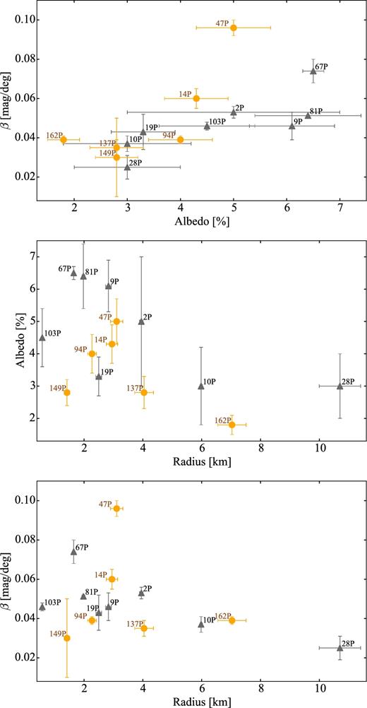
Surface properties of all JFCs with known radius, albedo and phase function. The orange circles correspond to comets with properties derived in this work. Top: phase function slope versus albedo. There is a trend of increasing phase function slope with increasing albedo. Comet 47P was active at the time of the observations, so in reality its phase function coefficient might be smaller and its albedo might be higher. Middle: albedo versus radius. Bottom: phase function coefficient versus radius.
We note a possible correlation between the phase function coefficient and the albedo in Fig. 62 (top panel). It is well established that similar correlations exist between albedo or spectral type and phase functions for asteroids (e.g. Oszkiewicz et al. 2012).
Comet 47P was determined to be active at the time of the observations that were used to determine its albedo and phase function. Under these conditions, it is possible that we have overestimated the nucleus brightness and therefore underestimated its albedo. Additionally, the activity possibly led us to determine an inaccurate phase function. Due to these concerns, we prefer to exclude it from the analysis.
We performed a Spearman rank correlation test between the phase function coefficient and the albedo of all comets (excluding 47P). The test produced rank ρ of 0.82 and p-value of 0.0005 which suggests a possible correlation between the phase function coefficients and albedos. In order to confirm this possible correlation and to be able to interpret it, we need to increase the number of JFCs with well-determined surface properties.
6 SUMMARY
We have developed a method for precise absolute calibration of photometric time series using Pan-STARRS DR1 stars. With this technique we achieved photometric calibration with uncertainty as low as 0.02 mag. Thus, we were able to study the rotation, shapes, and surfaces of nine JFCs, most of which were observed at multiple epochs using different instruments. We have collected an up-to-date sample of JFCs with published rotational properties and expanded it with the measurements from this work. We used the extended sample to characterize the bulk properties of JFCs. The results are as follows:
We have used time series photometry of nine JFCs taken in the period 2004–2015 to study their light curves. We have derived the rotation rates of six comets (14P, 47P, 93P, 94P, 110P and 162P). For comets 123P, 137P and 149P, the collected data were insufficient to derive unambiguous rotation periods. To our knowledge, for comets 93P, 94P and 162P these are the first published rotation rates. Comets 14P, 47P and 110P had previous light curves but our results significantly improved the period estimates.
Lower limits on the axial ratios of all observed comets have been derived from the brightness variation of the time series. Three of the comets, 47P, 93P and 123P, were most likely active at the times of the observations and therefore their brightness variation was most likely underestimated.
We have determined the linear phase function coefficients of seven of the observed comets – 14P, 47P, 94P, 110P, 137P, 149P and 162P. To our knowledge, for all comets except 47P, this is the first phase function determination. Our results have increased the number of comets with well-constrained phase function coefficients from 13 to 19.
The derived phase function coefficients have been used in the calculation of the absolute magnitudes Hr(1, 1, 0). For comets 93P and 123P, we used a phase function coefficient β = 0.04 mag deg−1. All comets except for 110P were part of SEPPCoN and had radius measurements derived from Spitzer infrared observations (Fernández et al. 2013). Using these radii and the derived absolute magnitudes, we have estimated the albedos of all eight comets.
We derived a geometric albedo of 1.8 ± 0.3 per cent for comet 162P. This makes 162P the JFC with lowest measured geometric albedo to date.
Prior to this work, there were nine comets for which both the albedo and the phase function coefficient were known (see Snodgrass et al. 2011). We have updated the values for 47P and added five more comets (14P, 94P, 137P, 149P, 162P) to this sample.
The increased number of comets has allowed us to look for correlations between the surface properties of JFCs. Large nuclei (Reff ≥ 5 km) appear to have low albedos (≤3 per cent) and low phase function coefficients (≤0.04 mag deg−1). However, since only three comets in that size range have been observed, this needs to be confirmed with future observations. We have discovered a possible correlation between the phase function coefficient and the albedo, where comets with larger albedos have steeper phase functions. In order to confirm as well as to interpret this result, we would require further phase function observations.
In Table 5, we have collected the known albedos and phase functions of 24 JFCs. The distribution of the linear phase function slopes has a median of 0.046 mag deg−1 and standard deviation of 0.017 mag deg−1. The known albedos have a median of 4.2 per cent and standard deviation of 1.3 per cent
We have reviewed the properties of all JFCs which (to the extent of our knowledge) had published rotation rates. After adding the six comets from this work, the total size of the sample has reached 37 comets.
We have attempted to use the distribution of spin rates to improve the understanding of JFC evolution. The employed Kolmogorov–Smirnov tests determined that the normalized spin rates of comets are consistent both with a Maxwell distribution and a flat distribution. Therefore, we cannot distinguish between the possibilities that JFCs are a collisionally dominated population-like asteroids or their spin rate distribution is dominated by other processes, such as activity-driven spin changes.
The distribution of the axial ratios shows that the majority of comets have projected axial ratios smaller than 2. The median of the whole JFC sample is 1.5. However, ground observations only give a lower limit to the axial ratio. All five comets with shape models determined from in situ spacecraft observations have axial ratios larger than 1.6.
Under the assumption that JFCs have negligible tensile strengths, we have used their axial ratios and periods to constrain their bulk densities. We have confirmed the result from Lowry & Weissman (2003) that a density of 0.6 g cm−3 is sufficient to keep all of the studied nuclei stable against rotational instabilities.
If we instead model JFCs as prolate ellipsoids with non-negligible tensile strengths using the model from Davidsson (2001), we conclude that none of the observed comets requires tensile strength higher than 10–25 Pa in order to be stable against rotational splitting. Comet 73P-C lies very close to the stability limit we derived, which suggests that its ongoing splitting might be due to rotational instabilities. An interesting outcome of this analysis is that comet 31P also lies very close to the stability limit which makes it a candidate for potential future splitting.
Acknowledgements
We would like to thank the referee, Imre Toth, for the helpful suggestions that improved the manuscript. This work is based on observations collected at the European Organisation for Astronomical Research in the Southern Hemisphere under ESO programmes 072.C-0233(A), 074.C-0125(A), 077.C-0609(B), 079.C-0297(A), 079.C-0297(B), 082.C-0517(A), 082.C-0517(B), 089.C-0372(A), 089.C-0372(B) and 194.C-0207(C). We thank the observatory staff who helped us obtain the various data sets in this paper, especially those collected in service mode at the VLT. Also based on observations made with the WHT and INT operated on the island of La Palma by the Isaac Newton Group of Telescopes in the Spanish Observatorio del Roque de los Muchachos of the Instituto de Astrofisica de Canarias, under UK PATT programmes I/2005A/11, W/2007A/20 and W/2008B/23.
CS is funded by an STFC Ernest Rutherford fellowship. AF acknowledges support from STFC grant ST/L000709/1.
The Pan-STARRS1 Surveys (PS1) and the PS1 public science archive have been made possible through contributions by the Institute for Astronomy, the University of Hawaii, the Pan-STARRS Project Office, the Max-Planck Society and its participating institutes, the Max Planck Institute for Astronomy, Heidelberg and the Max Planck Institute for Extraterrestrial Physics, Garching, The Johns Hopkins University, Durham University, the University of Edinburgh, the Queen's University Belfast, the Harvard-Smithsonian Center for Astrophysics, the Las Cumbres Observatory Global Telescope Network Incorporated, the National Central University of Taiwan, the Space Telescope Science Institute, the National Aeronautics and Space Administration under Grant No. NNX08AR22G issued through the Planetary Science Division of the NASA Science Mission Directorate, the National Science Foundation Grant No. AST-1238877, the University of Maryland, Eotvos Lorand University (ELTE), the Los Alamos National Laboratory, and the Gordon and Betty Moore Foundation.
REFERENCES
