


Abstract
Submillimetre galaxies (SMGs) are some of the most luminous star-forming galaxies in the Universe; however, their properties remain hard to determine due to the difficulty of identifying their optical/near-infrared counterparts. One of the key steps to determining the nature of SMGs is measuring a redshift distribution representative of the whole population. We do this by applying statistical techniques to a sample of 761 850 μm sources from the Submillimetre Common User Bolometer Array 2 Cosmology Legacy Survey observations of the UKIDSS Ultra-Deep Survey (UDS) field. We detect excess galaxies around >98.4 per cent of the 850 μm positions in the deep UDS catalogue, giving us the first 850 μm selected sample to have virtually complete optical/near-infrared redshift information. Under the reasonable assumption that the redshifts of the excess galaxies are representative of the SMGs themselves, we derive a median SMG redshift of z = 2.05 ± 0.03, with 68 per cent of SMGs residing between 1.07 < z < 3.06. We find an average of 1.52 ± 0.09 excess K-band galaxies within 12 arcsec of an 850 μm position, with an average stellar mass of 2.2 ± 0.1 × 10¹⁰ M⊙. Whilst the vast majority of excess galaxies are star forming, 8.0 ± 2.1 per cent have passive rest-frame colours and are therefore unlikely to be detected at submillimetre wavelengths even in deep interferometry. We show that brighter SMGs lie at higher redshifts, and use our SMG redshift distribution – along with the assumption of a universal far-infrared Spectral Energy Distribution (SED) – to estimate that SMGs contribute around 30 per cent of the cosmic star formation rate density between 0.5 < z < 5.0.
1 INTRODUCTION
Submillimetre wavelengths are well suited to studying high-redshift galaxies, since redshift effects combine with the steep Rayleigh–Jeans tail of the dust spectral energy distribution resulting in negative K-corrections. This ensures that galaxies of a fixed far-infrared (far-IR) luminosity (a proxy for star formation rate) are approximately equally bright from z = 1 out to z = 6 (e.g. Blain et al. 2002).
The low resolution of submillimetre observations with even the most widely used cameras – the Submillimetre Common User Bolometer Array (SCUBA; Holland et al. 1999) on the 15 m James Clerk Maxwell Telescope, and the Large APEX BOlometer CAmera (LABOCA; Siringo et al. 2009) on the APEX 12 m telescope – and high-redshift nature of submillimetre galaxies (SMGs) make identifying their counterparts (i.e. the sources responsible for the submillimetre emission) challenging (e.g. Ivison et al. 2007), particularly in deep optical observations. Whilst the tight far-IR radio correlation (e.g. Helou, Soifer & Rowan-Robinson 1985; Yun, Reddy & Condon 2001; Jarvis et al. 2010; Smith et al. 2014) and low sky density of radio sources (e.g. Condon et al. 2012), allow the unambiguous identification of many SMG counterparts using high-resolution radio observations (e.g. Ivison et al. 2002, 2005, 2007), this is still a challenging undertaking, despite the current availability of sensitive radio data over degree-scale fields. This means that the most fundamental requirement for inferring the properties of SMGs – their redshift distribution – is hard to measure (e.g. Smail et al. 2002). Chapman et al. (2005) obtained spectroscopic redshifts to 73 SMGs based on following up 98 out of 104 radio-identified SMGs in a parent sample of 150 > 3σ SCUBA 850 μm sources, whilst Wardlow et al. (2011) were able to robustly identify only 72 out of 126 SMGs (an identification rate of 57 per cent) detected in LABOCA observations of the ECDF-S field, using a combination of radio, 24 μm and Spitzer IRAC data. Recent advances have improved matters, but even the latest methods (e.g. the ‘tri-colour’ technique put forward by Chen et al. 2016) can identify reliable counterparts to only 69 ± 16 per cent of SMGs. This means that, although SMGs are undoubtedly some of the most rapidly star-forming systems in the Universe (e.g. Hayward et al. 2011, 2013a), optical/near-infrared studies of their counterparts and therefore redshifts have so far been incomplete.
At the same time, several studies had attempted to complete the redshift distribution of SMGs using longer wavelengths, for example, Koprowski et al. (2014), Koprowski et al. (2016) and Michałowski et al. (2017), which used an average SMG template from Michałowski, Hjorth & Watson (2010) to find the redshift giving the best fit to the far-IR/millimetre photometry. Of course, the redshifts produced using long wavelengths are in general less accurate than those produced from optical/near-infrared data (although the latter are also highly uncertain at the highest redshifts). There are several reasons for this: for example, that far-IR data are susceptible to the influence of the choice of dust Spectral Energy Distribution (SED), and are subject to errors arising from blended far-IR photometry (e.g. Scudder et al. 2016, although – as in the aforementioned studies – this may be mitigated using deblending techniques such as those from Merlin et al. 2015 or Hurley et al. 2017). On the other hand, this method of redshift estimation does benefit from not requiring an optical/near-infrared counterpart, is able to obtain individual redshifts for every source and is also potentially less susceptible to the influence of chance alignments between optical sources, e.g. lensing.
Given the low resolution of submillimetre data based on single-dish observations, interferometers have an important role to play for studying SMGs. Some of the first results using sensitive data from the Atacama Large Millimetre Array (ALMA) to identify the counterparts to SMGs by Hodge et al. (2013) showed using a combination of radio and mid-IR data that ∼80 per cent of SMGs are identified correctly, but with completeness of just 45 per cent. Interferometry has also shown that many SMGs have multiple counterparts; whilst Barger et al. (2012) found that 37.5 per cent of bright SMGs are multiples (albeit with a 1σ confidence interval between 17 and 74 per cent), Hodge et al. (2013) found that at least 35 per cent of SMGs are multiples, whilst Chen et al. (2013) used the Submillimeter Array (SMA) to determine a lower multiple fraction of |$12.5^{+12.1}_{-6.8}$| per cent, and this value is likely to be affected by the sample selection (e.g. the flux limit). Multiplicity is also a key parameter if we are to clarify the role of SMGs within current models of galaxy formation and evolution; however, it presents considerable challenges for traditional cross-identification efforts (e.g. using likelihood ratio methods; Wolstencroft et al. 1986; Sutherland & Saunders 1992; Smith et al. 2011; Fleuren et al. 2012). The properties of SMGs are therefore still under investigation, using both observations (e.g. with large amounts of time allocated to investigate the source counts and multiplicity with the ALMA; Hodge et al. 2013; Karim et al. 2013; Carniani et al. 2015; Simpson et al. 2015; Fujimoto et al. 2016; Oteo et al. 2016; Dunlop et al. 2017) and simulations (e.g. can theory produce sufficiently star-forming galaxies, or are chance alignments required? Davé et al. 2010; Hayward et al. 2013b; Cowley et al. 2015; Muñoz Arancibia et al. 2015).
New technology used by the Submillimetre Common User Bolometer Array 2 (hereafter SCUBA-2; Holland et al. 2013) has given us unprecedented mapping speed at these wavelengths, meaning that we can now efficiently survey large areas. As a result, the SCUBA-2 Cosmology Legacy Survey (CLS; Geach et al. 2017) has surveyed ∼5 deg2 to better than mJy depth, increasing the total known sample of 850 μm sources by an order of magnitude. The extensive efforts to cross-identify these sources at other wavelengths highlight that they are critical if we are to understand the properties of SMGs, and their high redshift, dusty nature means that the K-band data in the UKIDSS UDS (Hartley et al. 2013) are ideal for this purpose. With sensitive ancillary data covering the rest-frame UV, optical and near-infrared (UVOIR) bands, we can also estimate the redshifts and stellar masses of possible counterparts, as well as classify them on the basis of their rest-frame colours. Williams et al. (2009) identified regions in the rest-frame (U − V) versus (V − J) – hereafter ‘UVJ’ – space believed to contain predominantly passive and star-forming galaxy populations, and this method is widely used (e.g. Whitaker et al. 2012; Hatch et al. 2014; Leja et al. 2015; Mendel et al. 2015; Fumagalli et al. 2016; Rees et al. 2016).
In this paper, we statistically study the optical/near-infrared properties of galaxies around the positions of a large sample of submillimetre sources taken from the CLS. Wardlow et al. (2011) and Simpson et al. (2014) made attempts to statistically identify those SMGs that could not be cross-identified using other means in the ECDF-S field; however, the ancillary data in those works were not deep enough to detect counterparts to the full SMG sample (whilst the former work detected counterparts to 85 per cent of their SMG sample, the latter found only 0.61 ± 0.07 counterparts per ALMA-blank SMG). Given the availability of the largest samples of submillimetre positions from the CLS and the deepest K-band data from the Ultra-Deep Survey (UDS), we now extend this idea to infer the properties of the whole 850 μm selected sample, complementary to the aforementioned long-wavelength estimates of the complete SMG redshift distribution, most recently by Michałowski et al. (2017).
In Section 2, we introduce the data sets used in our analysis, and explain how our sample was selected, whilst Section 3 contains our results, which we discuss in Section 4, before concluding with Section 5. We adopt a standard cosmology with ΩM = 0.3, |$\Omega _\Lambda = 0.7$|, H0 = 71 km s−1 Mpc−1, whilst all magnitudes and colours are quoted on the AB system (Oke & Gunn 1983).
2 DATA AND SAMPLE SELECTION
We base our analysis on the 850 μm data from the CLS observations of the UKIDSS UDS field. The CLS 850 μm data reduction is described in Geach et al. (2017), and the UDS field is centred on α = 02h17m46s, δ = −05°05΄15″ (J2000), covering an area of 0.8 deg2 with a median rms ∼0.88 mJy beam−1. We use the catalogue of SMGs in the CLS-UDS maps from Geach et al. (2017), which contains 1088 SMGs detected at >3.5σ.
The UDS data release 8 (Hartley et al. 2013) has a 5σ depth of K = 24.6 within 2 arcsec apertures over a field of 0.8 deg2. Over the central 0.6 degree2 of this field, the DR8 catalogue includes matched photometry in the UBVRi΄z΄JHK, 3.6 μm and 4.5 μm bands (measured using the method given in Simpson et al. 2012), ideal for estimating galaxy colours. We use the high-quality (|$\Delta z \backslash (1+z) \sim 0.031$|) photometric redshifts from Hartley et al. (2013), alongside stellar mass estimates and rest-frame colours estimated using the fast code (Kriek et al. 2009), which will be fully described in Smith et al. (in preparation). We derive these assuming an initial mass function from Chabrier (2003), based on the stellar SEDs from Bruzual & Charlot (2003), with exponentially declining star formation histories, a range of metallicities (0.2 < Z/Z⊙ < 2.5), a range of 0.0 < AV < 5.0 (assuming a dust law from Calzetti et al. 2000) and correcting for extinction in our own galaxy. Rest-frame colours for galaxies are estimated by convolving the best-fitting BC03 spectra found by fast with the Bessel U- and V-band curves (Bessell 1990) and with the Mauna Kea J-band filter curve (Tokunaga, Simons & Vacca 2002) in the rest frame. These values allow us to locate galaxies within the UVJ diagram, in which passive galaxies are those which have (U − V)rest > 1.3, (V − J)rest < 1.6 and (U − V)rest > 0.88 × (V − J)rest + 0.49.
We limit the influence of bright stars and UDS image artefacts (e.g. detector cross-talk) by removing all sources which are flagged in the UDS masks, supplied on the UDS website.1 In addition, we remove stellar sources from our sample by using the Bayesian classifications from Simpson et al. (2013). We limit our area to the region where the UDS data include photometric redshifts, and after removing regions masked in the UDS catalogue, the effective area of our survey is 0.527 deg2 in which we find 761 SMGs from the Geach et al. (2017) catalogue. We also remove those sources with χ2 > 20 in either the Hartley et al. (2013) or fast SED fitting to limit the influence of bad fits on photometric redshifts, galaxy colours and stellar masses.
3 RESULTS
In contrast to other investigations on this subject, we do not attempt to identify individual counterparts to CLS submillimetre sources. Instead, we take a statistical approach by measuring the properties of galaxies detected within and immediately around the SCUBA-2 beam, after subtracting off the expected background population, as a function of search radius. This method has the benefit of not requiring any assumptions about the number of K-band sources around each individual 850 μm position, and in the coming sections we will show that this enables us to generate a complete redshift distribution for 850 μm sources based on the UDS optical/near-infrared photometric redshifts. However, the price that we pay for this is that we do not identify the counterparts to any individual 850 μm source, and we also suffer from the issue that, because the environments of 850 μm sources have been shown to be overdense by a factor of 80 ± 30 times the background level (Simpson et al. 2015), the excess galaxies that we see in the near-infrared may not be responsible for the submillimetre emission themselves (see Section 3.4 below).
3.1 Astrometry and initial checks
Before searching around the 850 μm source positions for K-band galaxies, we must first ensure that the CLS and UDS positions are consistent with each other. We do this by following the method used for sources in the Herschel-ATLAS survey by Smith et al. (2011), which involves creating a two-dimensional histogram of the difference between the 850 μm and UDS positions for every source in each catalogue, which is shown in Fig. 1. Each bin of the hi-stogram is 1 arcsec in size and reveals a residual offset in the 850 μm astrometry relative to the UDS. To make the best estimate of the magnitude and direction of the offset, we model this distribution using a simple three-component model, consisting of two Gaussians with a common centre, plus a constant background, and find the best-fitting values for the centroid. The best-fitting offsets derived using this model are Δα = 1.41 ± 0.15 arcsec and Δδ = −0.95 ± 0.14 arcsec, giving an effective offset of 1.7 arcsec (i.e. smaller than the pixel size in the 850 μm maps), which we apply to the CLS catalogue before continuing.
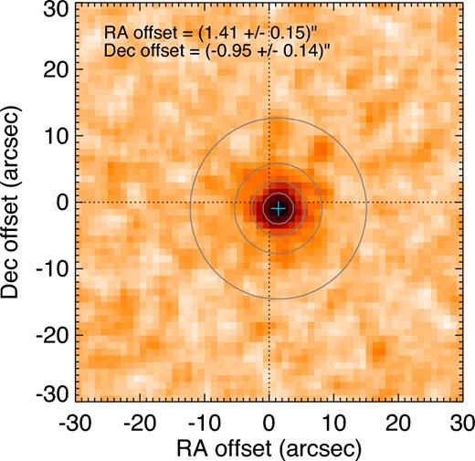
Image showing a two-dimensional histogram of the differences between the 850 μm positions of the 761 sources in our catalogue and the K < 24.6 UDS positions. The dotted lines indicate zero offset in the horizontal and vertical directions, whilst the blue cross indicates the best-fitting centroid position, as detailed as in the legend. The grey circles indicate the contours of the best-fitting double-Gaussian model used to determine the best-fitting centroid, with levels corresponding to 0.01, 0.1, 0.2 and 0.5 times the peak value.
3.2 The fraction of 850 μm sources detected in the UDS catalogue
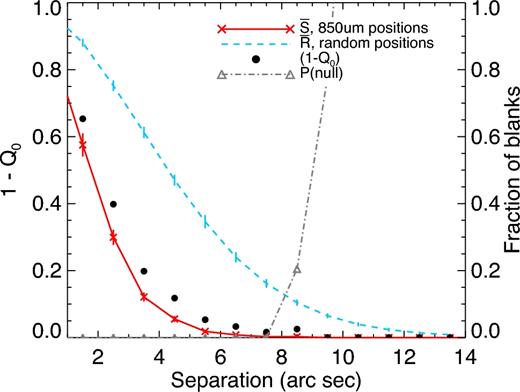
Illustration of the procedure of Fleuren et al. (2012) to estimate (1 − Q0), the fraction of 850 μm sources which are not detected in the UDS catalogue. The red crosses show the fraction of blanks (i.e. those 850 μm positions with no possible counterpart within the search radius), whilst the light blue dashed line shows the corresponding values based on random positions, both relative to the right-hand vertical axis. The black filled circles represent the values obtained dividing the number of blanks by the randomly generated values, which is our estimate of (1 − Q0), relative to the left-hand axis. The grey dot–dashed line linking the triangles indicates the probability of obtaining the number of blanks around the 850 μm source positions by chance, and this is <1 per cent at all separations ≤10 arcsec. The values for Q0 and the probability of the null hypothesis are shown in Table 1.
Tabulated values of Q0 as a function of maximum separation from the 850 μm source positions, with the right-hand column showing the probability of obtaining our results by chance, after accounting for the fraction of sources in the >3.5σ 850 μm catalogue which are spurious.
| Max separation | Q0 | Pnull |
|---|---|---|
| (arcsec) | ||
| 1 | 0.103 | 0.000 |
| 2 | 0.346 | 0.000 |
| 3 | 0.602 | 0.000 |
| 4 | 0.802 | 0.000 |
| 5 | 0.882 | 0.000 |
| 6 | 0.947 | 0.000 |
| 7 | 0.967 | 0.000 |
| 8 | 0.984 | 0.000 |
| 9 | 0.975 | 0.205 |
| 10 | 1.000 | 0.780 |
| Max separation | Q0 | Pnull |
|---|---|---|
| (arcsec) | ||
| 1 | 0.103 | 0.000 |
| 2 | 0.346 | 0.000 |
| 3 | 0.602 | 0.000 |
| 4 | 0.802 | 0.000 |
| 5 | 0.882 | 0.000 |
| 6 | 0.947 | 0.000 |
| 7 | 0.967 | 0.000 |
| 8 | 0.984 | 0.000 |
| 9 | 0.975 | 0.205 |
| 10 | 1.000 | 0.780 |
3.3 The K < 24.6 galaxy population around 850 μm sources
Having ascertained that the UDS data are deep enough that almost every CLS 850 μm source has at least one detectable (if not identifiable) and associated K < 24.6 galaxy, we now wish to estimate how many galaxies we find for each. We do this by calculating the number of possible counterparts within a range of search radii between 0 and 20 arcsec, and subtract off the number of unassociated background sources that we would expect based on scaling the source density in the UDS K-band catalogue to the relevant search area. The results are shown in Fig. 3, in which the red points with Poisson error bars show the radial distribution of the number of excess galaxies around the 761 850 μm sources. For comparison, we also overlay the corresponding plot based on 1000 Monte Carlo simulations of the hypothetical scenario with one counterpart galaxy for each 850 μm position, assuming normally distributed positional uncertainties depending solely on the signal-to-noise ratio (SNR) of each source in the CLS catalogue (following the method in Ivison et al. 2007), added in quadrature with the 2 arcsec uncertainty resulting from pixel-quantized positions in the public CLS catalogue. We overlay the median-likelihood values (black) on the 16th and 84th percentiles of the cumulative frequency distribution (in grey) as a function of separation. We observe that the number of excess galaxies increases steadily out to around 12 arcsec, giving an average of 1.52 ± 0.09 excess K < 24.6 galaxies around each 850 μm source. These values highlight that in many cases we are detecting an excess of nearby K-band galaxies rather than the sources responsible for the 850 μm emission; this number is therefore not directly analogous to the SMG ‘multiplicity’ discussed above, but assuming that it is not dominated by a handful of sources with many components (and our estimate of Q0 derived in Section 3.2 suggests that this is a reasonable assumption), finding 1.52 ± 0.09 excess galaxies per 850 μm position is in good agreement with more direct studies of SMG multiplicity, both observationally (e.g. Chen et al. 2016) and using simulations (e.g. Hayward et al. 2013b).
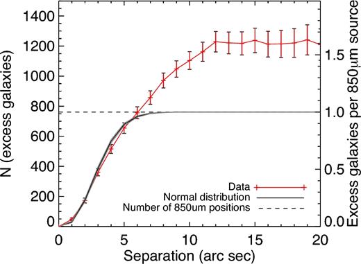
The radial distribution of excess galaxies around the CLS 850 μm positions (red points with error bars), compared with expectations based on a single counterpart per SMG assuming normally distributed positional offsets depending on the SNR, following Ivison et al. (2007), shown as the solid black line with grey region indicating the 16th and 84th percentiles of the expected excess based on our Monte Carlo simulations. Whilst the left-hand vertical axis shows the total number of excess galaxies around the sample of 761 850 μm sources in our search area, the right-hand axis has been scaled to show the average number of excess K-band galaxies around each source. The horizontal dashed line shows the number of 850 μm sources in our catalogue.
3.4 The properties of galaxies near 850 μm sources
We characterize these galaxies by extending the method of Section 3.3 to produce background-subtracted distributions of their photometric redshifts, K-band magnitudes and stellar masses, and these are shown in Fig. 4. To determine the extent to which the properties of these sources are representative of the SMG host galaxy population, we perform an identical analysis using realistic mock catalogues based on lightcones from the Bolshoi simulation (Klypin, Trujillo-Gomez & Primack 2011), containing galaxies with stellar mass >109 M⊙ over 0.5 < z < 8.0, which were produced by Hayward et al. (2013b) to study SMGs. Whilst the stellar masses of excess galaxies within 12 arcsec of 850 μm sources in the Bolshoi simulation (selected to the same flux criterion as in the real CLS catalogues) are significantly different from the stellar masses of the SMGs themselves, a Kolmogorov-Smirnov (K-S) test shows that we are unable to rule out the hypothesis that the redshift distributions are drawn from the same parent distribution (we perform this simulation 1000 times and find a median P ≈ 0.3). We therefore conclude that the photometric redshift distribution derived in this manner is representative of the full SMG population.
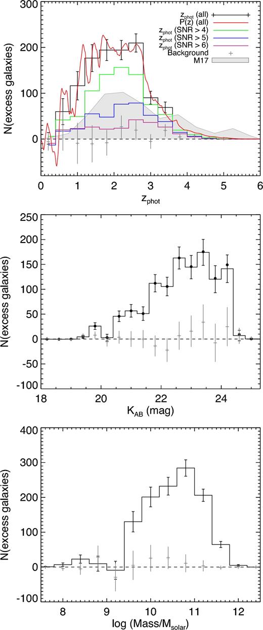
The properties of the galaxies within 12 arcsec of 850 μm sources including, Top: photometric redshift distribution (which our simulations suggest is indistinguishable from the redshift distribution of SMGs), Middle: K-band magnitude distribution and Bottom: best-fit stellar mass distribution. In each panel, the grey points with error bars show the results of applying the same background subtraction method to the same number of random search radii as there are CLS 850 μm sources in our survey area, with the error bars estimated from propagating the Poisson errors on each individual data point. In the top panel, we also overlay the photometric redshift distribution from Michałowski et al. (2017, shown as the grey shaded region), and those that we have produced for brighter subsets of the SMG population, detected at >4σ, >5σ and >6σ, shown as green, blue and purple histograms, respectively. We also overlay the corresponding summed P(z) derived based on the individual redshift probability distributions for each source (in red). In the middle panel, the black filled circles show the same data as the error bars, but corrected for residual completeness in the UDS catalogue, derived using the corrections from Mortlock et al. (2015).
In the top panel of Fig. 4, we show the photometric redshift distribution of the 1154.6 ± 67.5 excess galaxies around all 761 >3.5σ CLS 850 μm sources in our survey area as the black histogram, derived from the best-fitting redshifts from the Hartley et al. (2013) catalogue, and overlaid (in red) with the corresponding distribution derived from the individual redshift probability distribution functions. The median redshift of the 850 μm sources is 〈z〉 = 2.05 ± 0.03, which makes for an interesting comparison with many previous studies despite their incomplete redshift information (e.g. Wardlow et al. 2011; Casey et al. 2013; Simpson et al. 2014; Chen et al. 2016) and despite the important role played by selection (which we will discuss in Section 4.2). We find that 18.2 per cent of the SMGs in our sample lie at z > 3, in good agreement with Wardlow et al. (2011). We also overlay the results of performing an identical analysis on the same number of random positions as the grey error bars, which recover a redshift distribution consistent with zero excess galaxies, reassuring us that our results are not caused by some undiagnosed bias. We have overlaid our results on the redshift distribution for the ≥4σ sample of SMGs selected from the CLS observations of the COSMOS and UDS fields from Michałowski et al. (2017), who (as discussed in Section 1) completed the redshift distribution for the ∼third of sources without cross-identified counterparts in their sample using long-wavelength data. The Michałowski et al. (2017) redshift distribution (which has been arbitrarily rescaled for clarity) has a higher median |$\langle z \rangle = 2.40^{+0.10}_{-0.04}$|, and this is most readily apparent in the increased high-redshift tail in the shaded grey distribution in the top panel of Fig. 4. This apparent disagreement between the two >4σ source redshift distributions (shaded grey from Michałowski et al. 2017, corresponding to the green distribution from this work) is of particular interest given the complementary strengths and weaknesses of the two methods.
Though the Bolshoi simulation shows that the mass distribution of the galaxies in the simulation around the 850 μm source positions differs from the mass distribution of the model SMG counterparts, it is nevertheless instructive to calculate the K-band magnitude and stellar mass distributions of these sources. In the middle panel of Fig. 4, we show the distribution of K-band magnitude for the excess galaxies, overlaid with the results of the analogous experiment using the same number of random positions (grey error bars). Interestingly, rather than increasing towards the limit of the UDS catalogue, the magnitude distribution peaks around K = 23.4 mag (∼1.2 mag above the K = 24.6 mag limit) before turning down. This reinforces our result from Section 3.2 that the UDS data are sensitive enough to detect an excess of galaxies around virtually all of the 761 850 μm sources in the Geach et al. (2017) catalogue for which we have coverage. If the excess K-band galaxies that we detect are not the sources responsible for the 850 μm emission, the magnitude distribution of SMG counterparts must be bimodal, as expected based on the extreme dust columns around bright SMGs found by Simpson et al. (2015, |$A_V \approx 540^{+80}_{-40}$| mag). The fact that we are detecting galaxies around 850 μm sources not necessarily responsible for the 850 μm emission offers a possible means to reconcile our results with the fact that 5 out of the 30 > 8 mJy CLS submillimetre sources in Simpson et al. (2016) do not have a K-band counterpart to at least one of the multiple blended components resolved by ALMA in this field.
To test for the possible influence of incompleteness in our K-band catalogue on our magnitude distribution, we correct the K-band magnitude distribution using the completeness curve for the parent UDS DR8 catalogue from Mortlock et al. (2015), and the results of applying this correction are overlaid as the black filled circles, which are consistent with the original results. In the bottom panel of Fig. 4, we show the corresponding mass distribution. We find that galaxies around SMGs have an average stellar mass of 2.2 ± 0.1 × 10¹⁰ M⊙, around a factor of 2 lower than the value found by Wardlow et al. (2011, after accounting for the different initial mass function used in that work), though as noted above, that work assumed a standard H-band mass-to-light ratio for the stellar mass estimation, and was unable to account for the whole 850 μm source population, whilst we are likely biased towards lower stellar masses by including SMG neighbours in our calculation.
Since we derived rest-frame colours for every source in the UDS catalogue, we are able to apply the same technique to determine the locations of the excess galaxies around SMGs in the UVJ colour space. The results of doing so are shown in Fig. 5, in which the left-hand panel shows the distribution of galaxies in the UDS catalogue, with a dashed line to highlight the division between the regions occupied by star-forming and passive galaxies at z > 1, taken from Hartley et al. (2013). The colour of each bin is chosen to indicate the logarithm of the number of sources in that bin, ranging from 5 to 100 galaxies. In the right-hand panel, we show the corresponding colour–colour space for galaxies within 12 arcsec of a CLS 850 μm source, with the same colour scaling, highlighting that whilst the vast majority are classified as star forming on the basis of their rest-frame colours, a small subset (an excess of 92.8 ± 23.7, or 8.0 ± 2.1 per cent of the total galaxy excess) are consistent with being passive galaxies, in agreement with previous work on smaller samples of the SMGs themselves (Smail et al. 2004).2
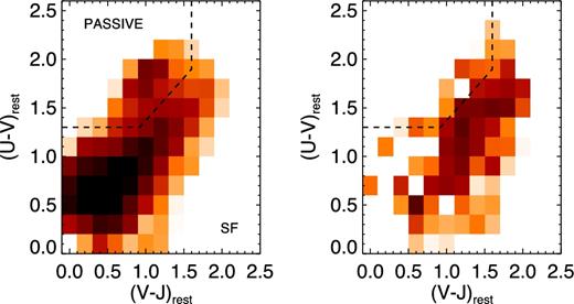
Left: the distribution of KAB < 24.6 galaxies within the UVJ colour–colour space from Williams et al. (2009), which is designed to separate passive and star-forming galaxies. The histograms are normalized to the area around all 761 850 μm sources in our sample and coloured according to the log of the bin occupancy, with values ranging from 5 to 100 galaxies per bin. The right-hand panel shows the UVJ colours of those K < 24.6 galaxies within 12 arcsec of a CLS 850 μm source, with the same colour scale as the left-hand panel.
These results make a particularly interesting comparison with the results of Smith et al. (in preparation), who find that the average 850 μm flux density of z > 1, K-selected and UVJ star-forming galaxies increases with increasingly red (V − J)rest colour, meaning that we expect many SMG neighbours to be submillimetre faint, and therefore very difficult to identify even using, e.g. sensitive high-resolution submillimetre observations with ALMA, and the same is of course true of the passive galaxies. This highlights the need for deep optical/near-infrared data alongside sensitive interferometry if we are to truly understand the relationship between the properties of SMG host galaxies and their environments.
4 DISCUSSION
4.1 Can we believe photometric redshifts for sources this faint?
In deriving these results, we have of course assumed some degree of reliability in the UDS photometric redshifts, which Hartley et al. (2013) showed to be very precise. However, this can only be verified using spectroscopy, which is extremely challenging to obtain for large samples of faint sources such as those studied here, and the lower-left panel of Fig. 4 indicates that ∼39 per cent of the galaxies associated with 850 μm positions are fainter than K = 23.0, the limit of the UDSz spectroscopic sample selection (Almaini et al., in preparation).
Meanwhile, some works in the literature (e.g. Simpson et al. 2014) have been reluctant to quote photometric redshifts for sources with formal detections (defined as having an SNR > 3σ) in fewer than four optical/near-infrared bands, taking the conservative view that photometric redshifts derived for such sources are unreliable. However, other works have shown the value of measurements for deriving galaxy parameters even when they are not formally significant (e.g. Smith et al. 2013, 2014), and this is one of the reasons why photometric redshift codes such as fast (Kriek et al. 2009) and lephare (Ilbert et al. 2006) ideally require measured flux densities rather than magnitudes in their input catalogues (since fluxes are symmetric even for faint sources, and allow noisy negative flux estimates to be naturally included in the fitting).
Since we have not directly identified any counterparts to the 850 μm sources, it is difficult to directly investigate the number of photometric detections for any individual source. However, we can repeat our analysis, this time including only those sources which have at least four >3σ detections in the UDS catalogue, and see what difference this makes to our results. We are still able to detect at least one galaxy associated with every SMG (i.e. our estimate of Q0 is still consistent with unity), and we still detect a significant excess of 1091.8 ± 66.8 galaxies, as compared with 1154.6 ± 67.5 when the full sample is considered. This change indicates that around 5 per cent of the galaxies around SMGs have fewer than four 3σ detections, but the significance of the change is <1σ, based on propagating the Poisson error bars. The average photometric redshift of the excess galaxies around SMGs in the remaining sample is 1.99 ± 0.03, which is consistent with the original value of 2.05 ± 0.03, whilst the UVJ passive fraction in the excess galaxies is unchanged. We therefore suggest that whilst this aspect may play a minor role, it does not give us any cause to mistrust our results more than we would any other study using photo-z; our approach benefits once more from not relying on any one single photometric redshift.
4.2 Do the brightest SMGs differ from the rest?
Several previous investigations (e.g. Ivison et al. 2002; Pope et al. 2005; Biggs et al. 2011; Chen et al. 2016) have found evidence for differences between the brightest and faintest SMGs in terms of their redshifts and the number of sources contributing to the single-dish 850 μm flux density (though Wardlow et al. 2011, found no evidence for this). In Fig. 6, we show how the median redshift varies as a function of the 850 μm flux density as red error bars, ranging from the full sample to increasingly brighter subsets (note that the leftmost error bar is derived based on the whole population, with increasingly smaller subsets as we move towards brighter SNRs). Also overlaid are results from other selected observational works in the literature (Chapman et al. 2005; Wardlow et al. 2011; Casey et al. 2013; Vieira et al. 2013; Simpson et al. 2014; Chen et al. 2016; Michałowski et al. 2017) along with their quoted error bars. We have also overlaid an estimate based on the latest measurements of the far-IR luminosity function using SCUBA-2 and ALMA data from Koprowski et al. (2017), shown as the dot–dashed light blue line) and theoretical results for bright (>5 mJy) SMGs based on the galform semi-analytic model presented in Cowley et al. (2015), and based on the simulations from Hayward et al. (2013a).
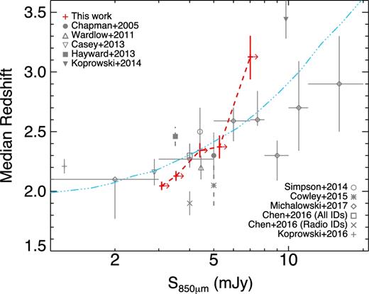
Variation in the average SMG redshift as a function of 850 μm flux density. Red error bars (connected with the dashed red line) are derived based on our sample, using the median statistics method of Gott et al. (2001), whilst the right-facing arrows are to indicate that each data point includes all sources at higher SNR. Also overlaid are the average redshifts measured by selected works in the literature, detailed in the legend. Observational works are shown with solid error bars, whilst theoretical studies are indicated by dashed error bars. Also overlaid, as a light blue dot–dashed line, is a prediction based on the latest estimate of the far-IR luminosity function out to z = 5 (Koprowski et al. 2017).
We find strong evidence for a higher median redshift for increasingly bright 850 μm sources in our sample, with error bars estimated from the redshift histograms using the median statistics method of Gott et al. (2001). The average redshift ranges from 2.05 ± 0.03 for the full SNR > 3.5σ sample (equivalent to a 3 mJy selected sample due to the highly uniform 850 μm map) of 761 galaxies to 3.13 ± 0.18 for the 45 sources brighter than 8σ. This result becomes even clearer if we consider the values quoted by other surveys, although the scatter in those works is considerably larger due to the smaller sample sizes with the exception of Michałowski et al. (2017), who calculated the average redshift in bins of 850 μm flux density, including the ultrafaint sample from Koprowski et al. (2016); these values are also overlaid in Fig. 6. The brightest samples, including the S1.1mm > 4.2 mJy SMGs from Koprowski et al. (2014) over the COSMOS field (corresponding to 850 μm flux >9.8 mJy assuming a standard dust SED) with 〈z〉 = 3.44 ± 0.16 and S1.4mm > 20 mJy SMGs (corresponding to 850 μm fluxes ≳100 mJy) observed by the South Pole Telescope, which have an average redshift of 3.5 according to both Vieira et al. (2013) and Weiß et al. (2013) further underline this trend.
In Fig. 7, we show a similar analysis, this time calculating the average number of galaxies around 850 μm positions as a function of SNR/flux. Taking the error bars into account, the data reveal little or no evidence for an increasing number of excess K < 24.6 galaxies towards brighter flux densities. This is reassuring, since if brighter 850 μm sources had a significantly larger number of excess galaxies, this might have skewed our photometric redshift distribution given that brighter sources lie at higher redshifts (Fig. 6).
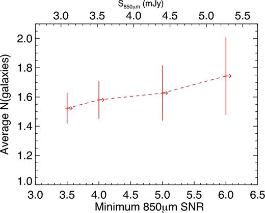
The variation in the average number of K < 24.6 galaxies within 12 arcsec of an 850 μm position, as a function of the 850 μm SNR. As in Fig. 6, the upper horizontal axis has been converted to 850 μm flux density assuming a uniform uncertainty of 0.88 mJy, the median value of sources in the CLS 850 μm map of the UDS field.
It is of course possible that strongly gravitationally lensed sources within the 850 μm selected population could artificially increase the number of excess galaxies observed around the 850 μm positions, and previous works have shown that bright submillimetre flux selection can efficiently identify such systems (e.g. Negrello et al. 2010). However, according to the latest results, lensed systems only contribute appreciably to the 850 μm number counts above fluxes of 20 mJy (Geach et al. 2017), and there are no sources this bright in our sample. Since Fig. 7 also shows little evidence for an increase in the average number of excess galaxies for the brightest sources in our sample, we therefore suggest that strongly lensed galaxies do not have a major influence on our results.
4.3 The contribution of SMGs to cosmic star formation
In Fig. 8, we bring all of this information together, in an attempt to measure the contribution of SMGs to the cosmic star formation rate density (SFRD) estimates from Behroozi, Wechsler & Conroy (2013, shown as the dashed line) and Madau & Dickinson (2014, dotted line). We do this by randomly assigning redshifts to the 850 μm sources by sampling from the cumulative frequency distribution of photometric redshifts, using the different distributions shown in the main panel of Fig. 4 (i.e. we ensure that we encode the behaviour apparent in Fig. 6). We can then convert the deboosted 850 μm flux density supplied in the CLS 850 μm catalogue (Geach et al. 2017) to a star formation rate (SFR) assuming an isothermal dust SED model (e.g. Hildebrand 1983; Smith et al. 2013) with T = 30 K and β = 1.5, and a standard relationship between far-IR luminosity and SFR from Kennicutt (1998) adapted for our choice of initial mass function such that SFR (M⊙ yr−1) ≈ 1.06 × 10⁻¹⁰(Ldust/L⊙). We estimate the SFRD in bins of redshift by calculating |$\sum \frac{\psi _i}{V_{\mathrm{max}}}$|, where ψi represents the SFR of the ith source in the sample, and Vmax – the maximum comoving volume within which that source could be detected – is calculated by determining the redshift at which the 850 μm source would become too faint to be included in our 3.5σ catalogue, accounting for the effective area of our survey, which is 0.527 deg2. The grey points show these raw results, and we are able to correct these values to account for the completeness and fraction of false positives using the values supplied for each source in the CLS 850 μm catalogue. The corrected values are shown as the black asterisks, with error bars assigned from repeating the redshift assignment process 1000 times, and counting the 16th and 84th percentiles of the resulting SFRD in each bin.

The contribution of the CLS 850 μm sources to the cosmic SFRD calculated by Behroozi et al. (2013) and Madau & Dickinson (2014), shown as the dashed and dotted lines, respectively. The raw SFRs scaled from the individual deboosted 850 μm flux densities from Geach et al. (2017), assuming an isothermal far-IR SED with T = 30 K and β = 1.5, are shown as the blue crosses, whilst the red asterisks show the results when we fold the Geach et al. (2017) estimates of completenesses and false detection rates for each 850 μm source into our calculations. The error bars are derived by measuring the 16th and 84th percentiles of the results of performing 1000 Monte Carlo realizations of sampling from the redshift distributions shown in Fig. 4. Also overlaid are the results from the 4 mJy SMG sample from Michałowski et al. (2017), shown as grey diamonds, the obscured contribution estimated from ALMA observations of the Hubble Ultra Deep Field by Dunlop et al. (2017), shown as grey triangles, and the SFRD estimated based on radiative transfer modelling of Herschel galaxies from Rowan-Robinson et al. (2016), shown as light grey squares.
Though we have assumed a single isothermal dust SED template to make the conversion from 850 μm flux density to SFR, under this assumption we find that our SMG sample with complete redshift information contributes 30.5 ± 1.2 per cent of the Behroozi et al. (2013) cosmic SFRD estimate between 0.5 < z < 5.0 (where the uncertainty on the value we quote has been derived solely on the basis of Monte Carlo sampling from the photometric redshift distribution, and does not contain any contribution from the large uncertainty associated with the choice of far-IR SED). This value is in excellent agreement with the 30 per cent estimated by Barger et al. (2012) based on SMGs’ radio luminosities, though it is 50 per cent higher than found by Michałowski et al. (2010), despite our use of a comparatively quiescent far-IR SED relative to some other common choices (e.g. those based on prototypical local galaxies such as M82 or Arp 220 from Polletta et al. 2007, or based on SMGs from Pope et al. 2008; Michałowski et al. 2010). However, using any of these templates would result in the apparent contribution of star formation in SMGs exceeding the total in our lowest redshift bin at 0.5 < z < 1. We are of course able to mitigate this behaviour by assuming a relationship between far-IR luminosity and dust temperature (as found by many other studies; e.g. Chapman et al. 2003; Hwang et al. 2010; Smith et al. 2013; Symeonidis et al. 2013; Swinbank et al. 2014), though given that we have not identified individual counterparts to the submillimetre sources, it is difficult to directly address the Herschel properties of the counterparts in this work; however, this will be possible in future studies with complete x-IDs and fully deblended Herschel photometry.
Also overlaid in Fig. 8 are the SFRDs calculated based on the obscured star formation attributed to galaxies with SFR > 300 M⊙ yr−1 from Michałowski et al. (2017, grey diamonds), and the corresponding larger estimate of the total dust-obscured star formation based on the latest ALMA results (reconstructing the relationship between obscured SFR and stellar mass) using deep observations of the Hubble Ultra Deep Field by Dunlop et al. (2017, grey triangles). The comparison between the latter study and our results is of particular interest, since together the two studies imply that roughly 60 per cent of the total dust-enshrouded star formation over 1 < z < 4.5 is captured in SMGs detected by SCUBA-2. We have also included the results derived based on a 500 μm selected sample of sources obtained from 20 deg2 of Herschel data from Rowan-Robinson et al. (2016, as light grey squares), although as the authors note, they detect a far larger cosmic SFRD than in other works. This discrepancy underlines the power of SCUBA-2 for high-redshift studies.
Finally, we note that despite the uncertainty over the far-IR SED, we have reached our plausible results with the largest SMG sample with complete redshift information, and having naturally accounted for the fraction of 850 μm sources which are broken up into multiple components in high-resolution submillimetre interferometry, even if those components are widely separated in redshift.
5 CONCLUSIONS
We have used 761 850 μm sources from the SCUBA-2 CLS observations of the UKIDSS UDS field (Geach et al. 2017) alongside the 8th UDS data release (Hartley et al. 2013) to statistically measure the complete redshift distribution of 850 μm sources. Whilst our method is unable to identify the counterparts to individual SMGs, we are able to account for multiple neighbouring galaxies and for the distribution of background sources using the rich ancillary data that are available over this field.
We find that the UDS data are sufficiently deep to detect excess galaxies around virtually all of the 761 850 μm sources in our survey area, though we do not identify them, and they are not necessarily the same galaxies responsible for the 850 μm emission (some of which are too faint to be detected even in the UDS K-band data; Simpson et al. 2016). Simulations based on model lightcones suggest that the redshift distribution of excess galaxies within 12 arcsec of an 850 μm source is indistinguishable from that of the SMGs themselves, and we use this fact to measure their complete optical/near-infrared photometric redshift distribution, finding that the SMGs in our >3.5σ sample have an average redshift of 2.05 ± 0.03. We find an average of 1.52 ± 0.09 excess galaxies within 12 arcsec of an 850 μm position, and use the rest-frame colours of these galaxies to show that whilst the majority are likely to be dusty star-forming galaxies, a substantial fraction are likely to be submillimetre faint, passive galaxies, and therefore difficult to detect even in deep high-resolution submillimetre imaging, e.g. with ALMA. We show that the brightest SMGs lie at higher redshifts than the rest of the SMG population, and under the assumption of a universal isothermal far-IR dust spectral energy distribution, we find that SMGs contribute around 30 per cent of the cosmic SFRD between 0.5 < z < 5.0.
Acknowledgements
The authors would like to thank the referee, Jim Dunlop, for useful suggestions that have increased the quality of this paper. We are also grateful to Will Hartley and Omar Almaini for providing the UDS catalogue used in this work, as well as to Kristen Coppin, Jim Geach and Wendy Williams for valuable discussions. The James Clerk Maxwell Telescope has historically been operated by the Joint Astronomy Centre on behalf of the Science and Technology Facilities Council of the United Kingdom, the National Research Council of Canada and the Netherlands Organisation for Scientific Research. The James Clerk Maxwell Telescope is operated by the East Asian Observatory on behalf of The National Astronomical Observatory of Japan, Academia Sinica Institute of Astronomy and Astrophysics, the Korea Astronomy and Space Science Institute, the National Astronomical Observatories of China and the Chinese Academy of Sciences (Grant No. XDB09000000), with additional funding support from the Science and Technology Facilities Council of the United Kingdom and participating universities in the United Kingdom and Canada. Additional funds for the construction of SCUBA-2 were provided by the Canada Foundation for Innovation. The UKIDSS project is defined in Lawrence et al. (2007) and uses the UKIRT Wide Field Camera (Casali et al. 2007). The Flatiron Institute is supported by the Simons Foundation.
To convince ourselves that our background subtraction is working as expected, we inverted the data and replotted with the same colour scheme, revealing no significant galaxy excess.
REFERENCES
