


Abstract
We have carried out a campaign to characterize the hot Jupiters WASP-5b, WASP-44b and WASP-46b using multiband photometry collected at the Observatório do Pico Dos Dias in Brazil. We have determined the planetary physical properties and new transit ephemerides for these systems. The new orbital parameters and physical properties of WASP-5b and WASP-44b are consistent with previous estimates. In the case of WASP-46b, there is some quota of disagreement between previous results. We provide a new determination of the radius of this planet and help clarify the previous differences. We also studied the transit time variations including our new measurements. No clear variation from a linear trend was found for the systems WASP-5b and WASP-44b. In the case of WASP-46b, we found evidence of deviations indicating the presence of a companion but statistical analysis of the existing times points to a signal due to the sampling rather than a new planet. Finally, we studied the fractional radius variation as a function of wavelength for these systems. The broad-band spectrums of WASP-5b and WASP-44b are mostly flat. In the case of WASP-46b we found a trend, but further measurements are necessary to confirm this finding.
1 INTRODUCTION
Since the announcement of the discovery of the first exoplanets orbiting the pulsar PSR 1257+12 (Wolszczan & Frail 1992; Wolszczan 1994) and the subsequent discovery of an exoplanet around a main sequence star (Mayor & Queloz 1995), more than 3000 planets orbiting other stars have been detected (Schneider et al. 2011, see exoplanet.eu). An exoplanet's orbit oriented along the line of sight provides unmatchable access to a list of both planetary astrophysical properties and orbital elements. The favourable geometry of transiting extrasolar planets (TEPs) allows the measurement of the true planetary masses and radii provided some external constraints from stellar evolutionary theory or empirical stellar mass–radius relations (Southworth 2009). Moreover, if the stellar limb darkening is assumed to be negligible, the density of the star can be measured directly from the light curve alone (Seager & Mallén-Ornelas 2003). Additionally, some of the stellar light filters through the exoplanet atmosphere during transit, resulting in spectral footprints that may reveal characteristics of the exoplanetary atmosphere (e.g. Swain et al. 2010). TEPs allow for the first time to access an accurate ensemble of planetary properties; thus, the accurate characterization of each system plays an important role for both the determination of fundamental parameters and recognition of astrophysically interesting targets for follow-up work such as transit timing variation (TTV; Holman & Murray 2005; Holman et al. 2010) or atmospheric characterization (see e.g. Seager & Deming 2010).
Hot Jupiters (HJs) are a class of large and gaseous planets similar to Jupiter, but orbiting very close to their host stars. These characteristics make these objects easier to detect compared with low-mass planets at wider orbits. Despite the large number of HJs discovered, fundamental questions about their formation and evolution are still under debate. The main scenarios proposed to explain their tight orbital trajectories are the formation of orbits with a small inclination via disc migration, or very inclined orbits via high-eccentricity migration due to tidal dissipation caused by gravitational interactions with another companion (see e.g. Ford & Rasio 2008; Thies et al. 2011; Tutukov & Fedorova 2012; Valsecchi & Rasio 2014). Therefore, precise physical and geometrical parameters of HJs derived from optical and infrared photometry are essential to test the planetary formation and evolution theories as well as to distinguish different types of atmospheres (Sing et al. 2016).
In this paper, we present precision relative photometry of three HJs: WASP-5b, WASP-44b and WASP-46b (Anderson et al. 2008, 2012). WASP-5b is an HJ with a mass of MP = 1.64 MJ and a radius of RP = 1.17 RJ transiting a bright (V = 12.3 mag) G4V star on a 1.63 d orbit. WASP-44b has a mass of MP = 0.89 MJ and a radius of RP = 1.00 RJ orbiting a bright (V = 12.9 mag) G8V star with an orbital period of 2.42 d. WASP-46b is a massive (MP = 2.10 MJ) HJ with a radius of RP = 1.31 RJ eclipsing a bright (V = 12.9 mag) G6V star on a 1.43 d orbit.
This paper is structured as follows: Section 2 describes the observations and the data reduction, Section 3 presents our results and analysis, and in Section 4 we discuss our results and state our conclusions.
2 OBSERVATIONS AND DATA REDUCTION
The observations were carried out using the facilities of the Observatório do Pico dos Dias (OPD/LNA), in Brazil.1 Transits of the planets WASP-5b, WASP-44b and WASP-46b were observed on 2011 August, 2012 August, 2013 July and 2013 August using the Andor iKon-L CCD cameras mounted on the 1.6-m and 0.6-m telescopes. These cameras provide plate scales of 0.18 and 0.34 arcsec pixel−1, respectively. A summary of the collected data is reported in Table 1. In this table, N is the number of individual images obtained with integration time texp.
Summary of the photometric observations presented in this work.
| Target | ut date | N | texp (s) | Telescope | Filter | Aperture (pix) | Scatter (per cent)a | Slope spectrumb |
|---|---|---|---|---|---|---|---|---|
| WASP-5b | 2012 August 10 | 992 | 10 | 1.6-m | V | 16.0 | 0.23 | (1.73 ± 2.3) × 10−5 |
| 2012 August 10 | 362 | 40 | 0.6-m | IC | 9.0 | 0.26 | ||
| WASP-44b | 2012 August 11 | 296 | 60 | 1.6-m | V | 11.0 | 0.14 | |
| 2012 August 11 | 346 | 40 | 0.6-m | RC | 8.0 | 0.38 | ||
| 2012 August 11 | 200 | 60 | 0.6-m | IC | 5.0 | 0.40 | (−1.07 ± 11.1) × 10−6 | |
| 2012 August 16 | 230 | 60 | 1.6-m | B | 11.0 | 0.19 | ||
| 2013 August 01 | 832 | 08 | 1.6-m | IC | 7.0 | 0.24 | ||
| WASP-46b | 2011 August 14 | 300 | 30 | 1.6-m | V | 13.0 | 0.19 | |
| 2013 July 30 | 601 | 10 | 1.6-m | IC | 10.0 | 0.23 | (−2.31 ± 1.77) × 10−5 | |
| 2013 August 02 | 361 | 15 | 1.6-m | RC | 14.0 | 0.17 |
aStandard deviation of the residuals after subtracting the fitted model.
bSee Section 3.5.
The basic data reduction was done using iraf2 tasks. We created a master median bias of typically ∼100 bias frames for each observing night. A normalized master flat-field frame was obtained by combining and then normalizing ∼30 dome flat-field images. We process the images by subtracting the master bias and then dividing by the normalized master flat frame.
The target fields are not crowded; thus, we performed standard differential aperture photometry. The telescope tracking and pointing were not stable during the observations; thus, we carefully placed the apertures in each image for both the target and the reference non-variable stars. The fluxes were extracted using an implementation of daophot (Stetson 1987). We experimented with different apertures and sky rings and kept those which resulted in the lowest standard deviation after subtracting the fitted transit model (see next section). This was an efficient way of both measuring the fit quality, due to the reduced number of out-of-transit observations, and discarding outliers. We iteratively removed the outliers discarding measurements 3σ away from the resulting model light curve (see next section). We repeated this process up to three times for each band which resulted in a maximum of removal of 1.5 per cent of the data points and an average reduction of 10 per cent in the residuals standard deviation. The final aperture values used to extract our light curves are listed in Table 1.3
3 ANALYSIS AND RESULTS
3.1 Light-curve analysis
To fit the light curves we used exofast (Eastman, Gaudi & Agol 2013). This software implements the Markov Chain Monte Carlo (MCMC) method to estimate and characterize the parameters’ uncertainty distributions (Ford 2005, 2006) and the light-curve models of Mandel & Agol (2002). To evolve the MCMC chains, it uses the differential evolution MCMC method (Ter Braak 2006). We included at each MCMC step the background value at the central pixel, airmass and CCD positions; thus, ensuring these systematics are considered at each MCMC jump. In fact, these systematics were critical to fit properly our light curves in the cases of changes of the positions of our targets and references (see discussion below about our systematics). To include these parameters in the MCMC chains, we considered a linear combination of the (x, y) pixel positions of the target's star centroid, the airmass and the background value which was computed averaging the pixel values within a ring around the star. For each light curve, we ran MCMC chains of maximum 100 000 iterations and discarded the first 25 000 chains which eliminated any bias due to the starting conditions (‘burn-in’ process, Tegmark et al. 2004). To check their convergency, we divided the final 75 000 values into three, and computed the mean and standard deviation (best-fitting value and error) of the posterior distributions. If the derived values were consistent within 1σ errors, we considered the chains to be convergent. Since we fitted only transit data, we complemented our fits with spectroscopic information taken from Anderson et al. (2008, 2012) and Triaud et al. (2010). We fixed the eccentricities to zero, as the radial velocity data are consistent with circular orbits.
exofast uses a quadratic law to take into account the limb darkening. Southworth (2008) proved this law is sufficient to model high-quality ground-based light curves. We fitted both coefficients for each light curve. Espinoza & Jordán (2015) proved that this approach introduces bias just up to ∼1 per cent in RP/R*. exofast adds a penalty term at each MCMC jump based on the tables of Claret & Bloemen (2011), thus constraining the fitted limb-darkening coefficients and preventing their values to be unphysical.
We calculated the standard deviation of the measurements after subtracting the fitted model (scatter) to assess the quality of the fit. The final scatter values are displayed in Table 1.
Light curves of planetary transits have systematic effects, the so called correlated ‘red noise’ (Pont, Zucker & Queloz 2006). To quantify this noise, we used the residual permutation method (RPM; Jenkins, Caldwell & Borucki 2002) implemented in the transit analysis package jktebop (Southworth 2008). In this method, the residuals around the best fit are shifted point by point along the observations and a new fit is performed (if a residual is shifted after the end it is moved to the beginning). This is done for all observational data points. From the resultant distribution the errors are calculated as in the MCMC case. These uncertainties are a way to quantify the systematics present in our data. We found that the uncertainties determined by the RPM are in most cases similar to the MCMC case for the data taken with the 1.6-m telescope (there just a couple of extreme cases where the RPM uncertainties are slightly larger). In the case of data taken with the 0.6-m telescope, the RPM uncertainties are up to three times the MCMC uncertainties, so the systematics are stronger in this case. This is in part explained because the pointing of the 0.6-m telescope changes more drastically (drift of 90 pixels for every 20 min of observing time); thus, target and references are placed on different CCD positions, therefore increasing the systematics due to changes in quantum efficiency. Additionally, the 0.6-m has no guiding system. The 1.6-m telescope has a guiding system and therefore a better pointing. As pointed out before, these changes of position were taken into account at each MCMC iteration.
We also fitted the light curves with jktebop using MCMC simulations (using an approach similar to that of exofast). This served as a consistency check of our exofast results. We found the results to be consistent with each other within one standard deviation. We preferred exofast results because it implements at each MCMC jump a penalty term taking into account the decorrelation parameters. As stated before, taking into account the systematics present in our data is critical for improving the final results and to properly characterize the uncertainties. As a final consistency check, we also analysed our light curves using the graphical transit analysis interface Transit Analysis Package (TAP) (Gazak et al. 2012). We also found the results to be consistent with exofast within one standard deviation. This is expected, because TAP uses exofast (Gazak et al. 2012), but iterates the MCMC chains using a wavelet-based likelihood (Carter & Winn 2009). All the results presented in this paper come from the exofast results and the other tools were used just as an initial consistency check. Figs 1– 3 show the resultant light curves of WASP-5b, WASP-44b and WASP-46b, respectively. In all cases, the scatter of the residuals was better than 0.4 per cent.
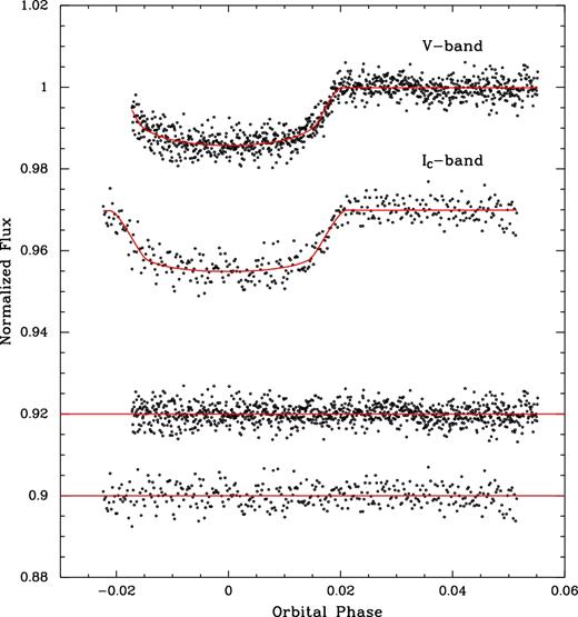
WASP-5b light curves. From top to bottom the V- and IC-band light curves, respectively. The red curves are the best fits superimposed. The residuals of the fitted model are displayed at the bottom. The displayed light curves are decorrelated using the parameters described in Section 3.1.
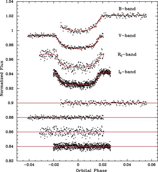
WASP-44b light curves. From top to bottom the B-, V-, RC- and IC-band light curves, respectively. The red curves are the best fits superimposed. The residuals of the fitted model are displayed at the bottom. The displayed light curves are decorrelated using the parameters described in Section 3.1.
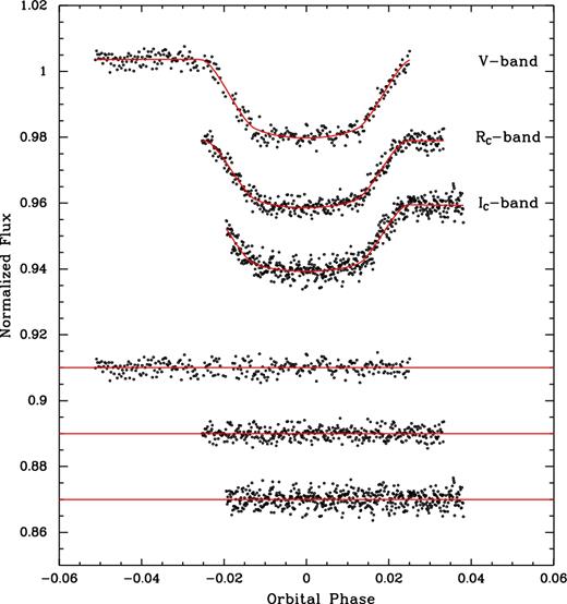
WASP-46b light curves. From top to bottom the V-, RC- and IC-band light curves, respectively. The red curves are the best fits superimposed. The residuals of the fitted model are displayed at the bottom. The displayed light curves are decorrelated using the parameters described in Section 3.1.
3.2 System parameters
Tables 2–4 show the determined parameters in all bands for the planets WASP-5b, WASP-44b and WASP-46b, respectively. As mentioned before, the quality of the light curves taken with the 1.6-m telescope is better, so we preferred those for IC-band results of WASP-44b. Thus, all the results presented in this paper refer to the IC band taken with the 1.6-m telescope for the WASP-44b system.
Planetary parameters of WASP-5b.
| Symbol | Parameter | V | IC |
|---|---|---|---|
| a | Semimajor axis (au) | |$0.02789_{-0.00058}^{+0.00059}$| | |$0.02793_{-0.00055}^{+0.00056}$| |
| RP | Radius ( RJ) | |$1.126_{-0.082}^{+0.100}$| | |$1.240_{-0.081}^{+0.085}$| |
| RP/R⋆ | Planet/star radius ratio | |$0.1114_{-0.0015}^{+0.0015}$| | |$0.1158_{-0.0017}^{+0.0018}$| |
| Teq | Equilibrium temperature (K) | |$1753_{-62}^{+70}$| | |$1765_{-62}^{+64}$| |
| 〈F〉 | Incident flux (109 erg s−1 cm−2) | |$2.14_{-0.29}^{+0.37}$| | |$2.21_{-0.29}^{+0.34}$| |
| TC | Time of mid-transit (BJDTDB − 2450000) | |$6150.61479_{-0.00056}^{+0.00050}$| | |$6150.61396_{-0.00057}^{+0.00054}$| |
| u1 | Linear limb-darkening coefficient | 0.484 ± 0.049 | |$0.285_{-0.050}^{+0.048}$| |
| u2 | Quadratic limb-darkening coefficient | 0.283 ± 0.052 | |$0.290_{-0.049}^{+0.048}$| |
| i | Inclination (deg) | |$86.1_{-1.4}^{+1.8}$| | |$84.54_{-0.66}^{+0.74}$| |
| δ | Transit depth | |$0.01155_{-0.00051}^{+0.00056}$| | |$0.01373_{-0.00052}^{+0.00053}$| |
| T14 | Total duration (d) | |$0.0978_{-0.0016}^{+0.0018}$| | |$0.0935_{-0.0023}^{+0.0025}$| |
Planetary parameters of WASP-44b.
| Symbol | Parameter | V | B | RC | IC |
|---|---|---|---|---|---|
| a | Semimajor axis (au) | 0.0352 ± 0.0014 | |$0.0328_{-0.0015}^{+0.0016}$| | 0.0354 ± 0.0016 | |$0.0349_{-0.0016}^{+0.0015}$| |
| RP | Radius ( RJ) | |$1.12_{-0.11}^{+0.10}$| | |$1.08_{-0.13}^{+0.15}$| | 1.18 ± 0.13 | |$1.121_{-0.081}^{+0.080}$| |
| RP/R⋆ | Planet/star radius ratio | |$0.1224_{-0.0013}^{+0.0013}$| | |$0.1346_{-0.0031}^{+0.0031}$| | |$0.1256_{-0.0032}^{+0.0033}$| | |$0.1246_{-0.0025}^{+0.0025}$| |
| Teq | Equilibrium temperature (K) | 1390 ± 120 | |$1200_{-100}^{+120}$| | |$1410_{-130}^{+140}$| | 1360 ± 120 |
| 〈F〉 | Incident flux (109 erg s−1 cm−2) | |$0.85_{-0.25}^{+0.33}$| | |$0.46_{-0.14}^{+0.23}$| | |$0.89_{-0.29}^{+0.40}$| | |$0.78_{-0.23}^{+0.31}$| |
| TC | Time of mid-transit (BJDTDB − 2450000) | |$6151.82559_{-0.00045}^{+0.00046}$| | |$6156.6694_{-0.0019}^{+0.0014}$| | |$6151.82415_{-0.00095}^{+0.0010}$| | 6505.70010 ± 0.00025 |
| u1 | Linear limb-darkening coefficient | |$0.493_{-0.084}^{+0.094}$| | |$0.932_{-0.12}^{+0.089}$| | |$0.378_{-0.089}^{+0.10}$| | |$0.331_{-0.070}^{+0.071}$| |
| u2 | Quadratic limb-darkening coefficient | |$0.222_{-0.088}^{+0.076}$| | |$-0.044_{-0.095}^{+0.12}$| | |$0.252_{-0.074}^{+0.066}$| | |$0.252_{-0.063}^{+0.061}$| |
| i | Inclination (deg) | |$86.13_{-0.58}^{+0.81}$| | |$86.89_{-0.85}^{+1.2}$| | |$85.85_{-0.60}^{+0.74}$| | |$86.23_{-0.48}^{+0.56}$| |
| δ | Transit depth | |$0.01501_{-0.00079}^{+0.00065}$| | |$0.0171_{-0.0014}^{+0.0015}$| | 0.0163 ± 0.0012 | |$0.01542_{-0.00070}^{+0.00071}$| |
| T14 | Total duration (d) | 0.0942 ± 0.0016 | |$0.0963_{-0.0038}^{+0.0042}$| | |$0.0937_{-0.0030}^{+0.0032}$| | |$0.09516_{-0.00095}^{+0.00099}$| |
Planetary parameters of WASP-46b.
| Symbol | Parameter | V | RC | IC |
|---|---|---|---|---|
| a | Semimajor axis (au) | 0.02421 ± 0.00052 | |$0.02414_{-0.00054}^{+0.00055}$| | 0.02407 ± 0.00055 |
| RP | Radius ( RJ) | |$1.338_{-0.062}^{+0.064}$| | |$1.230_{-0.051}^{+0.052}$| | |$1.209_{-0.072}^{+0.074}$| |
| RP/R⋆ | Planet/star radius ratio | |$0.1507_{-0.0017}^{+0.0017}$| | |$0.14109_{-0.00099}^{+0.00099}$| | |$0.1403_{-0.0022}^{+0.0021}$| |
| Teq | Equilibrium temperature (K) | |$1678_{-53}^{+51}$| | |$1657_{-52}^{+53}$| | 1641 ± 58 |
| 〈F〉 | Incident flux (109 erg s−1 cm−2) | |$1.80_{-0.22}^{+0.23}$| | |$1.71_{-0.20}^{+0.23}$| | |$1.65_{-0.22}^{+0.25}$| |
| TC | Time of mid-transit (BJDTDB − 2450000) | |$5788.52807_{-0.00030}^{+0.00032}$| | |$6506.57629_{-0.00025}^{+0.00023}$| | 6503.71529 ± 0.00034 |
| u1 | Linear limb-darkening coefficient | |$0.384_{-0.053}^{+0.055}$| | |$0.345_{-0.054}^{+0.055}$| | |$0.307_{-0.053}^{+0.054}$| |
| u2 | Quadratic limb-darkening coefficient | |$0.241_{-0.054}^{+0.053}$| | 0.275 ± 0.051 | |$0.287_{-0.052}^{+0.049}$| |
| i | Inclination (deg) | |$82.87_{-0.32}^{+0.34}$| | |$82.73_{-0.32}^{+0.33}$| | |$82.92_{-0.41}^{+0.46}$| |
| δ | Transit depth | |$0.02293_{-0.00076}^{+0.00082}$| | |$0.01976_{-0.00043}^{+0.00045}$| | |$0.01943_{-0.00095}^{+0.0010}$| |
| T14 | Total duration (d) | |$0.0727_{-0.0013}^{+0.0014}$| | |$0.06994_{-0.00094}^{+0.0010}$| | 0.0703 ± 0.0017 |
The inclination of the system and the orbital semimajor axis are independent of wavelength; thus, a unique value can be determined. We calculated a final value using as weight the inverse square of the individual uncertainties. Table 5 shows the results and previous estimates for the planets WASP-5b, WASP-44b and WASP-46b, respectively. Our values are consistent with previous results for these planets. We have improved the value of the inclination for WASP-5b and the normalized semimajor axis a/R* for WASP-46b.
Weighted mean of common parameters for WASP-5b, WASP-44b and WASP-46b.
| Parameter | This work | Southworth | Triaud et al. | Fukui et al. |
|---|---|---|---|---|
| (2009) | (2010) | (2011) | ||
| WASP-5b | ||||
| i (deg) | 84.77 ± 0.68 | 85.8 ± 1.1 | 86.2|$^{+0.8}_{-1.7}$| | 85.58|$^{+0.81}_{-0.76}$| |
| a/R* | 5.54 ± 0.19 | |$5.41^{+0.17}_{-0.18}$| | 5.49|$^{+0.37}_{-0.12}$| | 5.37 ± 0.15 |
| WASP-44b | ||||
| i (deg) | 86.18 ± 0.37 | 86.02|$^{+1.11}_{-0.86}$| | 86.59 ± 0.18 | |
| a/R* | 8.10 ± 0.20 | 8.05|$^{+0.66}_{-0.52}$| | 8.58 ± 0.3 | |$8.33^{+0.09}_{-0.14}$| |
| WASP-46b | ||||
| i (deg) | 82.82 ± 0.21 | 82.63 ± 0.38 | 82.80 ± 0.17 | |
| a/R* | 5.76 ± 0.09 | 5.74 ± 0.15 | 5.85 ± 0.12a | |
aValue calculated using the reported values of Ciceri et al. (2016) (propagating the lowest reported uncertainties for a and R*).
3.3 Transit ephemerides
3.4 Transit timing variations
The mid-transit times and the residuals from the fit are shown in Fig. 4 and listed in Tables 6–8. In the absence of TTVs (Holman & Murray 2005; Holman et al. 2010) we would expect no statistically significant deviations of the derived [O (observed) − C (calculated)] values from zero. To test the truthfulness of this we computed |$\chi ^2_{\rm red}$| for the three systems and found |$\chi ^2_{\rm red,WASP\text{-}5b}$| = 2.1, |$\chi ^2_{\rm red,WASP\text{-}44b}$| = 3.2 and |$\chi ^2_{\rm red,WASP\text{-}46b}$| = 61.8. Although the three values are sufficiently large to suspect the presence of TTVs, values around |$\chi ^2_{\rm red}\sim$|3 have created already some disagreement between authors (see e.g. von Essen et al. 2013 but then Mislis et al. 2015). None the less, WASP-46b's |$\chi ^2_{\rm red}$| value is large enough to suspect TTVs. To further investigate this we applied a Lomb–Scargle periodogram (Lomb 1976; Scargle 1982; Zechmeister & Kürster 2009) to the (O − C) values. The derived false alarm probabilities (FAP) are FAP|$_{\rm WASP\text{-}5b}$| = 0.64, FAP|$_{\rm WASP\text{-}44b}$| = 0.17 and FAP|$_{\rm WASP\text{-}46b}$| = 0.0002, placing again WASP-46b as a good candidate for TTVs. The power spectrum of WASP-46b's periodogram has a peak at 0.0034 ± 0.0004 c d−1 (cycles d−1), which corresponds to ∼295 d. The frequency and error were computed fitting a Gaussian profile to the maximum peak of the periodogram. As a measurement of the amplitude of WASP-46’s (O − C) diagram we used its standard deviation, with a value of 250.7 s. We finally re-determined the FAP of the TTV signal but using a bootstrap resampling method. For this, we randomly permuted the mid-transit values along with their errors 5× 10⁵ times, but leaving the epochs fixed. At each iteration we calculated a Lomb–Scargle periodogram from the permuted (O − C) diagram. We estimated the FAP as the frequency with which the highest power in the scrambled periodogram exceeds the maximum power in the original periodogram. Using this more reliable technique, the re-estimated FAP for WASP-46b is 0.04, inconsistent with the one computed in the usual way but still low. Finally, to characterize WASP-46b's TTVs we computed the spectral window of its (O − C) diagram. If the signal is associated with the sampling rather than to the true TTV signal, then the spectral window power spectrum should have a similar peak around 0.0034 c d−1. This was the case. We found one single and isolated peak at 0.0026 ± 0.0004 c d−1, just consistent with the previously computed TTV signal at the 1σ level (see Fig. 5). Although the TTV amplitude is significantly large, we notice that the more distant an (O − C) data point is from zero, the larger its error bar is. We therefore advise caution to readers who may want to interpret these TTVs.
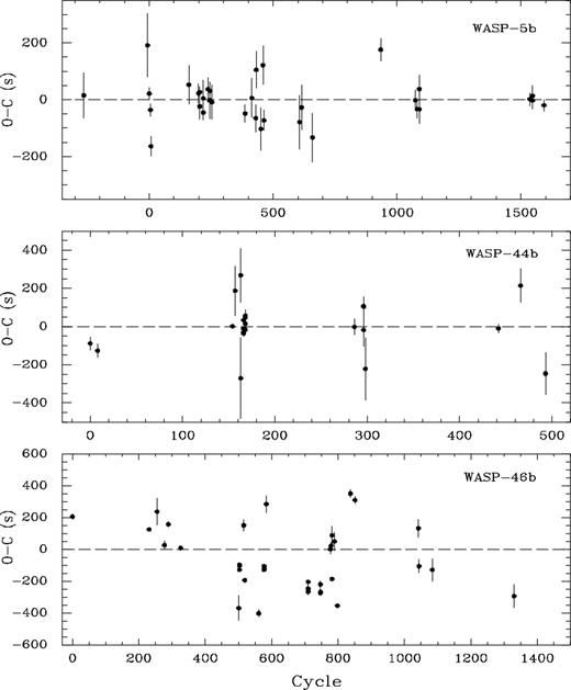
The panels from the top to bottom show the (O − C) diagrams for WASP-5b, WASP-44b and WASP-46b, respectively.
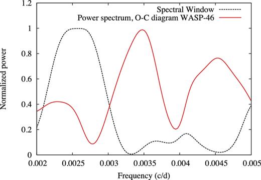
The figure shows, in a red continuous line, the periodogram of WASP-46 TTVs zoomed-in around the maximum power. On top of this, the spectral window (i.e. the periodicity induced by the sampling of the data) is plotted in black dashed lines. For a better comparison, both periodograms have been normalized to their respective maximum values.
Mid-transit times for WASP-5b.
| Cycle | T(BJDTDB) | (O − C) | Reference |
|---|---|---|---|
| 2450000 + | (s) | ||
| −264 | 3945.71962 ± 0.00093 | 15 | Gillon et al. (2009) |
| −7 | 4364.2283 ± 0.0013 | 191 | Gillon et al. (2009) |
| 0 | 4375.62535 ± 0.00026 | 22 | Gillon et al. (2009) |
| 5 | 4383.7675 ± 0.0004 | −36 | Anderson et al. (2008) |
| 7 | 4387.02275 ± 0.0010 | −164 | Anderson et al. (2008) |
| 160 | 4636.17459 ± 0.00079 | 53 | Fukui et al. (2011) |
| 199 | 4699.68303 ± 0.00040 | 22 | a |
| 204 | 4707.82523 ± 0.00023 | 26 | Southworth et al. (2009) |
| 204 | 4707.82465 ± 0.00052 | −23 | a |
| 218 | 4730.62243 ± 0.00031 | −45 | Southworth et al. (2009) |
| 218 | 4730.62301 ± 0.00075 | 5 | a |
| 237 | 4761.56356 ± 0.00047 | 37 | a |
| 244 | 4772.96212 ± 0.00074 | −2 | Fukui et al. (2011) |
| 245 | 4774.59093 ± 0.00030 | 31 | a |
| 253 | 4787.61792 ± 0.00069 | −9 | a |
| 387 | 5005.82714 ± 0.00036 | −49 | a |
| 414 | 5049.79540 ± 0.00080 | 6 | a |
| 430 | 5075.84947 ± 0.00056 | −64 | Dragomir et al. (2011) |
| 432 | 5079.10830 ± 0.00075 | 105 | Fukui et al. (2011) |
| 451 | 5110.04607 ± 0.00087 | −102 | Fukui et al. (2011) |
| 459 | 5123.07611 ± 0.00079 | 121 | Fukui et al. (2011) |
| 463 | 5129.58759 ± 0.00042 | −72 | a |
| 607 | 5364.0815 ± 0.0011 | −79 | Fukui et al. (2011) |
| 615 | 5377.10955 ± 0.00091 | −27 | Fukui et al. (2011) |
| 659 | 5448.75927 ± 0.0010 | −133 | Dragomir et al. (2011) |
| 934 | 5896.58124 ± 0.00046 | 177 | TRESCA |
| 1074 | 6124.55945 ± 0.00042 | −2 | TRESCA |
| 1082 | 6137.58653 ± 0.00037 | −33 | TRESCA |
| 1090 | 6150.61396 ± 0.00057 | −34 | This study |
| 1090 | 6150.61479 ± 0.00056 | 37 | This study |
| 1536 | 6876.89438 ± 0.00027 | 1 | TRESCA |
| 1547 | 6894.80707 ± 0.0003415 | −3 | TRESCA |
| 1547 | 6894.80726 ± 0.00042 | 14 | TRESCA |
| 1593 | 6969.71467 ± 0.00024 | −20 | TRESCA |
aHoyer, Rojo & López-Morales (2012).
Mid-transit times for WASP-44b.
| Cycle | T(BJDTDB) | (O − C) | Reference |
|---|---|---|---|
| 2450000 + | (s) | ||
| 0 | 5434.37637 ± 0.00040 | −89 | Anderson et al. (2012) |
| 8 | 5453.76639 ± 0.00042 | −127 | Anderson et al. (2012) |
| 154 | 5807.64374 ± 0.00013 | 1 | Mancini et al. (2013) |
| 157 | 5814.91731 ± 0.00150 | 187 | Evans P. (TRESCA) |
| 163 | 5829.45485 ± 0.00245 | −271 | Lomoz F. (TRESCA) |
| 163 | 5829.46110 ± 0.00163 | 268 | Lomoz F. (TRESCA) |
| 166 | 5836.72905 ± 0.00020 | −31 | Mancini et al. (2013) |
| 166 | 5836.72979 ± 0.00030 | 33 | Mancini et al. (2013) |
| 166 | 5836.72900 ± 0.00020 | −35 | Mancini et al. (2013) |
| 166 | 5836.72928 ± 0.00015 | −11 | Mancini et al. (2013) |
| 168 | 5841.57719 ± 0.00035 | 14 | Mancini et al. (2013) |
| 168 | 5841.57757 ± 0.00046 | 47 | Mancini et al. (2013) |
| 168 | 5841.57684 ± 0.00028 | −16 | Mancini et al. (2013) |
| 168 | 5841.57769 ± 0.00031 | 57 | Mancini et al. (2013) |
| 286 | 6127.58626 ± 0.00048 | −2 | Sauer T. (TRESCA) |
| 296 | 6151.82555 ± 0.00060 | 103 | This study |
| 296 | 6151.8242 ± 0.0010 | −18 | This study |
| 296 | 6151.82559 ± 0.00045 | 106 | This study |
| 298 | 6156.6694 ± 0.0017 | −222 | This study |
| 442 | 6505.7001 ± 0.0002 | −11 | This study |
| 466 | 6563.87407 ± 0.00102 | 213 | Evans P. (TRESCA) |
| 493 | 6629.31154 ± 0.00127 | −247 | René R. (TRESCA) |
Mid-transit times for WASP-46b.
| Cycle | T(BJDTDB) | (O − C) | Reference |
|---|---|---|---|
| 2450000 + | (s) | ||
| 0 | 5392.31628 ± 0.00020 | 206 | Anderson et al. (2012) |
| 231 | 5722.73197 ± 0.00013 | 125 | Ciceri et al. (2016) |
| 255 | 5757.06225 ± 0.00098 | 235 | TRESCA |
| 277 | 5788.52807 ± 0.00030 | 25 | This work |
| 289 | 5805.69409 ± 0.00020 | 157 | Ciceri et al. (2016) |
| 326 | 5858.61624 ± 0.00011 | 8 | Ciceri et al. (2016) |
| 501 | 6108.92750 ± 0.00091 | −370 | TRESCA |
| 503 | 6111.79133 ± 0.00011 | −103 | Ciceri et al. (2016) |
| 503 | 6111.79141 ± 0.00013 | −97 | Ciceri et al. (2016) |
| 503 | 6111.79132 ± 0.00013 | −104 | Ciceri et al. (2016) |
| 503 | 6111.79102 ± 0.00013 | −130 | Ciceri et al. (2016) |
| 516 | 6130.38914 ± 0.00042 | 150 | TRESCA |
| 519 | 6134.67627 ± 0.00016 | −195 | TRESCA |
| 561 | 6194.74962 ± 0.00027 | −402 | Ciceri et al. (2016) |
| 577 | 6217.63904 ± 0.00013 | −107 | Ciceri et al. (2016) |
| 577 | 6217.63892 ± 0.00011 | −117 | Ciceri et al. (2016) |
| 577 | 6217.63883 ± 0.00010 | −125 | Ciceri et al. (2016) |
| 577 | 6217.63877 ± 0.00012 | −130 | Ciceri et al. (2016) |
| 584 | 6227.65619 ± 0.00062 | 284 | TRESCA |
| 710 | 6407.87778 ± 0.00014 | −205 | Ciceri et al. (2016) |
| 710 | 6407.87730 ± 0.00033 | −246 | Ciceri et al. (2016) |
| 710 | 6407.87711 ± 0.00017 | −262 | Ciceri et al. (2016) |
| 710 | 6407.87705 ± 0.00021 | −268 | Ciceri et al. (2016) |
| 747 | 6460.80084 ± 0.00016 | −275 | Ciceri et al. (2016) |
| 747 | 6460.80090 ± 0.00020 | −270 | Ciceri et al. (2016) |
| 747 | 6460.80147 ± 0.00028 | −221 | Ciceri et al. (2016) |
| 747 | 6460.80092 ± 0.00025 | −269 | Ciceri et al. (2016) |
| 777 | 6503.71529 ± 0.00034 | 1 | This work |
| 779 | 6506.57629 ± 0.00025 | 23 | This work |
| 782 | 6510.86498 ± 0.00013 | −187 | Ciceri et al. (2016) |
| 782 | 6510.86816 ± 0.00067 | 87 | TRESCA |
| 789 | 6520.88034 ± 0.00067 | 49 | TRESCA |
| 798 | 6533.74905 ± 0.00013 | −354 | Ciceri et al. (2016) |
| 837 | 6589.54183 ± 0.00031 | 350 | TRESCA |
| 851 | 6609.56661 ± 0.00027 | 309 | TRESCA |
| 1042 | 6882.76617 ± 0.00065 | 131 | TRESCA |
| 1044 | 6885.62416 ± 0.00049 | −107 | TRESCA |
| 1084 | 6942.83890 ± 0.00083 | −130 | TRESCA |
| 1330 | 7294.70924 ± 0.00085 | −295 | TRESCA |
3.5 Broad-band spectrum
Multiband transit observations allow to study the fractional radii variation as a function of the wavelength. The planetary radius RP derived from transit observations may vary with the wavelength, as it can appear slightly larger when observed at wavelengths where the atmosphere contains strong opacity sources (Burrows et al. 2000; Seager & Sasselov 2000). These changes are at first approximation the broad-band transmission spectrum (e.g. Nikolov et al. 2013). We fitted our light curves again, but now we introduced as priors the calculated common parameters shown in Table 5 and the orbital periods. This improves the quality of the fractional radius determination. The improved results for this parameter are shown in Tables 2, 3 and 4 for WASP-5b, WASP-44b and WASP-46b, respectively. Figs 6–8 show the resulting fractional radii variation as a function of wavelength using our measurements (red squares) and the ones available in the literature (pink squares) for the planets WASP-5b, WASP-44b and WASP-46b, respectively. The horizontal error bars represent the full width at half-maximum of the used filters. The superimposed dotted green line in these figures is the linear fit using only our measurements constraining the fit to cross our measurement with the longest wavelength. We calculated the slopes of these lines to investigate some trends in our measurements. The values of the slopes are listed in Table 1.
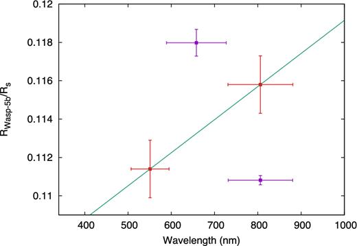
Planet to star radius of WASP-5b as a function of the observed band. The red squares are our measurements and the purple squares are the ones available in the literature. The green line is a linear fit to our measurements (see text).
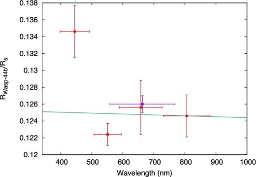
Planet to star radius of WASP-44b as a function of the observed band. Plotted as per the description for Fig. 6.
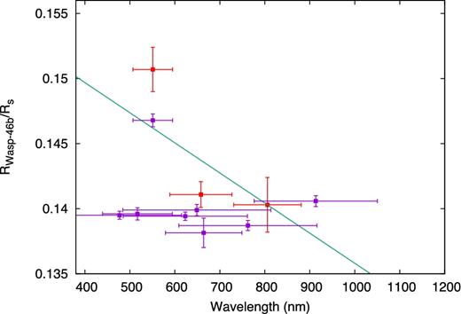
Planet to star radius of WASP-46b as a function of the observed band. Plotted as per the description for Fig. 6.
In the case of WASP-5b, there are not enough measurements to have an unambiguous view to describe a conclusive scenario for any correlation between the planetary radius and wavelength (e.g. Jha et al. 2000). In the case of WASP-44b, our values are consistent with a flat spectrum similar to that of Turner et al. (2016) (see their fig. 9). Our calculated slope (see Table 1) is consistent with zero. A flat spectrum is indicative of the presence of clouds in the upper atmosphere which prevent observation of any spectral features (Seager & Sasselov 2000; Turner et al. 2016). In the case of WASP-46b, we see indications of an increase of radius (4σ) at the shortest wavelengths, a hint of possible Rayleigh scattering in the atmosphere of this planet (Lecavelier Des Etangs et al. 2008). We notice that Ciceri et al. (2016) found no strong evidence of Rayleigh scattering in the atmosphere of WASP-46b (see their fig. 8). They found a slope with maximum inclination of m = −1.17 × 10⁻⁵ for WASP-46b (1/2 of our slope, see Table 1). Although there is rotational modulation on this system (Anderson et al. 2012), the stellar activity is not sufficient to explain this difference, so further measurements are necessary confirm or rule out this scenario. We also notice that the V-band light curve of WASP-46b is missing the flat part after egress (see Fig. 3), thus preventing from strongly constraining the baseline value, although our measurement is consistent within 2σ with that of Anderson et al. (2012). As pointed out by Gibson (2014), choosing an incorrect noise model might artificially lower the uncertainties which is equivalent to getting the normalization of the light curve wrong; thus, such high slope could be in part explained by the lack of observations after egress. We therefore advise caution to readers who may want to interpret this significant variation of the broad-band spectrum of WASP-46b. Although we recognize the V-band planetary to star radii ratio of WASP-46b is significantly larger than in the other bands, additional measurements will be needed to confirm this finding due to our lack of observations after egress.
As an alternative way of quantifying how much do the planetary to star radii ratio and wavelength correlate to each other, we made use of the Pearson's correlation coefficient, r. The derived values are as follows: rWASP-44b = −0.61, rWASP-46b = 0.11 and rWASP-5b = 0.05. These coefficients indicate that there is no correlation between the wavelength and planetary to star radii ratio for the systems WASP-5b and WASP-46b (values are close to zero). The coefficient rWASP-44b indicates that there is a significant anticorrelation for WASP-44b. In any case, we consider it unlikely that the amplitude of the variability in WASP-44b could vary with wavelength by more than 10 scaleheights, a sensible limit for expected variability when Rayleigh scattering is being investigated (Sing et al. 2016).
4 SUMMARY
In this paper, we have presented multiband photometry of three HJs: WASP-5b, WASP-44b and WASP-46b. The data were collected as part of an observational programme to characterize HJs which has been carried out with the facilities of the Pico dos Dias Observatory in Brazil. We performed a detailed analysis of the planetary transits using the following programmes: exofast (Eastman et al. 2013), TAP (Gazak et al. 2012) and jktebop (Southworth 2008). Using observations in the V, B, RC and IC bands, we were able to improve the geometrical and physical parameters of WASP-5b and WASP-46b (see Tables 2 and 4), in particular the ratio between the semimajor axis and the stellar radius for WASP-46b a/R* = 5.76 ± 0.09. The parameters we derived are consistent with previous studies (see Table 5)
We obtained improved linear ephemerides for WASP-5b, WASP-44b and WASP-46b using our mid-transit times measurements together with all the other measurements available in the literature (see Section 3.3). The analysis of the residuals from the linear fit, the (O − C) diagram, does not show a clear indication of TTV for WASP-5b and WASP-44b (see Fig. 4). The (O − C) diagram of WASP-46b shows variation with a semi-amplitude of ∼10 min. We proved this variation is most likely due to the sampling of the observations, but further additional transit time measurements of this system are necessary to secure this finding.
Finally, we studied the variation with wavelength of the planet to star radius for WASP-5b, WASP-44b and WASP-46b. We do not have enough measurements to describe the broad-band spectrum of WASP-5b. In the case of WASP-44b, our values are consistent with a flat spectrum similar to that of previous studies. In the case of WASP-46b, we found marginal evidence of Rayleigh scattering which is not in agreement with a previous study. Further measurements are necessary to confirm or rule out this finding.
Acknowledgments
MM thanks Joseph Carson and an anonymous referee for some helpful suggestions and for a critical reading of the original version of the paper. LAA acknowledges support from CAPES and Fundação de Amparo à Pesquisa do Estado de São Paulo – FAPESP (2013/18245-0 and 2012/09716-6). CvE acknowledges funding for the Stellar Astrophysics Centre, provided by The Danish National Research Foundation (Grant DNRF106).
The original light curves can be downloaded at http://www.iaucn.cl/Users/Max/PUBLIC/PAPER_OPD/
The TRansiting ExoplanetS and CAndidates (TRESCA) web-site can be found at http://var2.astro.cz/EN/tresca/index.php
REFERENCES
