


Abstract
We investigate the energy sources of random turbulent motions of ionized gas from H α emission in eight local star-forming galaxies from the Sydney-AAO Multi-object Integral field spectrograph (SAMI) Galaxy Survey. These galaxies satisfy strict pure star-forming selection criteria to avoid contamination from active galactic nuclei (AGNs) or strong shocks/outflows. Using the relatively high spatial and spectral resolution of SAMI, we find that – on sub-kpc scales, our galaxies display a flat distribution of ionized gas velocity dispersion as a function of star formation rate (SFR) surface density. A major fraction of our SAMI galaxies shows higher velocity dispersion than predictions by feedback-driven models, especially at the low SFR surface density end. Our results suggest that additional sources beyond star formation feedback contribute to driving random motions of the interstellar medium in star-forming galaxies. We speculate that gravity, galactic shear and/or magnetorotational instability may be additional driving sources of turbulence in these galaxies.
1 INTRODUCTION
The kinematics, structure and star formation activity of a galaxy depend on a combination of complex physical processes such as gravity, turbulence, magnetic fields, radiation, heating/cooling, feedback, accretion, operating both interior to and exterior to the galaxy. The relative importance of these processes is expected to depend on cosmic evolution and galactic environment. Galaxies at different cosmic epochs show quite distinct properties. Compared to their high-redshift counterparts at similar stellar masses, local star-forming galaxies are larger, and have relatively lower gas fractions and lower SFRs (Leroy et al. 2005; Daddi et al. 2010; Tacconi et al. 2010; Madau & Dickinson 2014). They are also less likely to experience violent events such as major mergers and gas accretion (Baugh, Cole & Frenk 1996; Genzel et al. 2008; Robotham et al. 2014).
Many theoretical and observational studies suggest that gas in higher redshift galaxies has larger random motions compared to gas in low-redshift galaxies (Nesvadba et al. 2006; Förster Schreiber et al. 2009; Lehnert et al. 2009, 2013; Wisnioski et al. 2015). These random, turbulent motions may play a crucial role in regulating the formation of stars (Green et al. 2010; Federrath & Klessen 2012; Padoan et al. 2014). However, the origin and energy source of the turbulence remain poorly understood. External mechanisms like gas accretion from the intergalactic medium and minor mergers (Glazebrook 2013), and internal mechanisms such as star formation feedback (stellar winds, supernovae), cloud–cloud collisions in the disc (Tasker & Tan 2009), the release of gravitational energy via accretion of cold gas streams from the halo or the inspiral of clumps (Klessen & Hennebelle 2010), galactic shear from the differential rotation in disc galaxies (Krumholz & Burkhart 2016), spiral-arms shocks in spiral galaxies, magnetorotational instability (MRI) (Tamburro et al. 2009) and others can potentially drive such turbulence (Mac Low & Klessen 2004; Elmegreen 2009; Federrath et al. 2016, 2017).
Several studies have been carried out to explore the energetic drivers of the turbulence in both high- and low-redshift disc galaxies, e.g. Elmegreen & Scalo (2004), Scalo & Elmegreen (2004), Tamburro et al. (2009), Gritschneder et al. (2009). Green et al. (2014) found that the gas velocity dispersion increases with SFR in star-forming galaxies both locally and at high redshift. Based on observations and analytic considerations, Lehnert et al. (2009, 2013) speculated that there is a relation between velocity dispersion and SFR surface density (ΣSFR) in active star-forming galaxies at z ∼ 1–3, and that it is the intense star formation that supports the high-velocity dispersion and thus balances the gravitational pressure. In contrast, Genzel et al. (2011) found that the velocity dispersion correlates only weakly with ΣSFR in their study of giant star-forming clumps in five galaxies at z ∼ 2 together with other rotation-dominant star-forming galaxies, lensed galaxies and dispersion-dominated galaxies at z ∼ 2. They suggest that a large-scale release of gravitational energy could induce the global large random motions in high-redshift galaxies, and that local star formation feedback triggering outflows and stirring up the interstellar medium (ISM) drives the local variation of turbulent, random motions.
Spatially resolved information is vital to understand the details of the physical processes that drive different interactions within galaxies. The three-dimensional (3D) spectra of galaxies uncover the distribution of the physical properties and give clues to how the internal physical processes shape the galaxies by connecting the spectral information with its position in the galaxy. Integral field spectroscopy (IFS) enables us to obtain this crucial spatial information. More importantly, IFS gives us both spectral and kinematic information; i.e. the intensity-weighted gas velocity and velocity dispersion along the line of sight. Taking advantage of this, IFS surveys such as the Calar Alto Legacy Integral Field Area Survey (CALIFA; Sánchez et al. 2012), the SAMI Survey (Croom et al. 2012; Bryant et al. 2015) and the Mapping Nearby Galaxies at Apache Point Observatory (MaNGA) Survey (Bundy et al. 2015) have made significant progress in this area. SAMI has a higher instrumental resolution σ = 29 km s−1 at 6250–7350 Å (Sharp et al. 2015) than the other IFS surveys mentioned above, which have instrumental resolution > 80 km s−1 at a similar wavelength range (Sánchez 2015). In this work, we investigate the properties of the ISM in star-forming galaxies using data from the SAMI Galaxy Survey. We measure maps of ΣSFR and gas velocity dispersion, and use these maps to derive the relation between ΣSFR and gas velocity dispersion. We further include ΣSFR and velocity dispersion data from the literature, and determine the dependence of velocity dispersion on redshift, up to z ∼ 3.
Section 2 presents the sample selection criteria and data reduction including the signal-to-noise ratio criteria, the data source and their reduction strategy, and the estimation of the magnitude of beam-smearing effect. In Section 3, our results and comparison with high-redshift and H α luminous local star-forming galaxies are presented. We further discuss the main source(s) of the turbulence in star-forming galaxies in Section 4. Section 5 summarizes the conclusions of this work. A standard cosmology of H0 = 70 km s−1 Mpc−1, Ωm = 0.3, ΩΛ = 0.7 is assumed throughout.
2 SAMPLE AND DATA ANALYSIS
2.1 Sample selection
2.1.1 The SAMI Galaxy Survey
We use the SAMI Galaxy Survey (Croom et al. 2012) to select local star-forming galaxies. The SAMI Survey will observe in total ∼3400 galaxies. It covers a broad range of galaxies in stellar mass and environment. The sample targets redshifts 0.004–0.095, Petrosian magnitudes rpet < 19.4,1 stellar masses 107–1012 M⊙ and environments from isolated field galaxies through group galaxies to cluster galaxies (Bryant et al. 2015; Owers et al. 2017).
SAMI is mounted at the prime focus on the Anglo–Australian Telescope. It has a 1° diameter field of view and uses 13 fused fibre bundles (Hexabundles; Bland-Hawthorn et al. 2011; Bryant et al. 2014) with a high (75 per cent) fill factor. Each of the bundles contains 61 fibres of 1.6 arcsec diameter that results in diameter of 15 arcsec in each integral field unit (IFU). The IFUs, together with 26 sky fibres, are inserted into pre-drilled plates using magnetic connectors. The SAMI fibres are fed to the double-beam AAOmega spectrograph (Sharp et al. 2006). AAOmega provides a range of different resolutions and wavelength ranges. For the SAMI Galaxy Survey, the 570 V grating at 3700–5700 Å is used to give a resolution of R = 1730 (σ = 74 km s−1), and the R1000 grating from 6250 to 7350 Å for a resolution of R = 4500 (σ = 29 km s−1) (Table 1) (Sharp et al. 2015). Therefore, each SAMI object has one blue and one red data cube. Early reduced data cubes are included in the first public data release (Allen et al. 2015, Green et al., in preparation). All data cubes are constructed on spatial grids where each grid cell has a size of 0.5 arcsec × 0.5 arcsec corresponding to a physical scale of ∼0.5 × 0.5 kpc2 for our sample of local star-forming galaxies (z ∼ 0.05). Note that the spatial resolution of SAMI data is determined by the average seeing in observations (∼2.5 arcsec), corresponding to a physical scale of 2.5 kpc (z ∼ 0.05).
Red and blue data cubes from LZIFU.
| Data cube | λa | Rb | σc |
|---|---|---|---|
| Blue | 3700–5700 Å | 1730 | 74 km s−1 |
| Red | 6250–7350 Å | 4500 | 29 km s−1 |
| Data cube | λa | Rb | σc |
|---|---|---|---|
| Blue | 3700–5700 Å | 1730 | 74 km s−1 |
| Red | 6250–7350 Å | 4500 | 29 km s−1 |
aWavelength range.
bSpectral resolution. Full width half-maximum (FWHM) = c/R.
cVelocity resolution according to spectral resolution.
The spectral fitting pipeline of SAMI galaxies, LZIFU (Ho et al. 2014, 2016), is designed to extract two-dimensional emission line flux maps and kinematic maps to investigate the dynamics of gas in galaxies. LZIFU uses up to three Gaussian profiles to fit emission lines, separating up to three different kinematic components contributing to the emission lines.
Maps of SFR and SFR surface density (Medling et al., in preparation) are also available in the SAMI data base. Briefly, these maps are calculated from extinction-corrected H α flux maps using the calibration in Kennicutt, Tamblyn & Congdon (1994). Extinction corrections are calculated using the Balmer decrement, and flux is converted to luminosity using distances calculated from the flow-corrected redshifts of the GAMA Survey Catalogue (Baldry et al. 2012).
2.1.2 Our sample
To select star-forming galaxies from the parent SAMI sample, we use optical emission line diagnostic diagrams, so-called BPT/VO diagrams (Baldwin, Phillips & Terlevich 1981; Veilleux & Osterbrock 1987) with multicomponent emission line fits. In the following analysis of the chosen star-forming galaxies, we use single component fits, which are sufficient to describe star-forming galaxies. In the most conservative way, we select those galaxies with all detected spaxels lying below the theoretical extreme starburst lines in all the three BPT/VO87 diagrams, i.e. [N ii] λ6583/H α versus [O iii] λ5007/H β, [S ii] λ6717, λ6731/H α versus [O i] λ6300/H β and [N ii] λ6583/H α versus [O iii] λ5007/H β (Baldwin et al. 1981; Veilleux & Osterbrock 1987; Kewley et al. 2001). Thus, we minimize the contamination of AGNs, outflows and shocks. We note that there are a few spaxels with elevated non-thermal-ratios suggestive of shocks in 508421. Because these spaxels are few in numbers and lie below the theoretical extreme starburst lines in all the three BPT/VO diagrams, we still keep this galaxy.
We find that 8 out of 756 SAMI galaxies satisfy our complete selection criteria. By the time of this work, 756 of the 3400 SAMI galaxies have had reduced data cubes available with the required analysis products. We find 22 star-forming galaxies meeting the criteria, but 11 of them are cluster galaxies that may be influenced by their environments. We choose not to discuss cluster galaxies, in order to focus on turbulence induced locally through accretion and/or galaxy-internal processes such as star formation feedback. Among the remaining 11 galaxies, two lack the information of stellar velocity dispersion (van de Sande et al. 2017, this will be relevant for a follow-up paper to determine the Toomre Q and that we want to use the same set of eight galaxies for this and the follow-up paper) and another lacks enough spaxels with high enough signal-to-noise ratio. Table 2 lists the basic information of the eight galaxies in our final sample. Our eight star-forming galaxies are at redshifts ranging from 0.017 to 0.055, most of them at the high end. Their stellar masses range from 6.3 × 10⁹ to 6.2 × 10¹⁰ M⊙ and the median stellar mass is 2.5 × 10¹⁰ M⊙, similar to most of the galaxies in the SAMI sample (Bryant et al. 2015).
Properties of the eight star-forming galaxies in our final sample of star-forming SAMI galaxies.
| CATID | RA | Dec. | Redshift | Stellar massa | Radiusb | Ellipc | id | σgase | ΣSFRf | |
|---|---|---|---|---|---|---|---|---|---|---|
| (hh: mm: ss) | (dd: mm: ss) | (M⊙) | (arcsec) | (kpc) | (°) | (km s−1) | (M⊙ yr−1 kpc−2) | |||
| 79635 | 14 50 03.3 | 43 51 03.1 | 0.040 | 2.9 × 10¹⁰ | 9.13 | 7.8 | 0.40 | 55.0 | 28 ± 4 | 0.019 ± 0.009 |
| 376001 | 08 46 31.3 | 00 05 51.0 | 0.051 | 1.8 × 10¹⁰ | 2.41 | 2.7 | 0.07 | 22.4 | 31 ± 9 | 0.022 ± 0.007 |
| 388603 | 09 23 08.1 | 02 29 09.9 | 0.017 | 6.3 × 10⁹ | 14.3 | 5.2 | 0.12 | 28.6 | 24 ± 4 | 0.009 ± 0.003 |
| 485885 | 14 31 01.9 | −01 43 02.0 | 0.055 | 1.8 × 10¹⁰ | 5.04 | 6.0 | 0.16 | 33.6 | 24 ± 4 | 0.014 ± 0.005 |
| 504882 | 14 30 15.3 | −01 55 56.2 | 0.054 | 1.3 × 10¹⁰ | 3.80 | 4.4 | 0.19 | 37.0 | 20 ± 2 | 0.010 ± 0.003 |
| 508421 | 14 27 57.4 | −01 37 52.3 | 0.055 | 2.5 × 10¹⁰ | 3.74 | 4.5 | 0.26 | 43.0 | 87 ± 44 | 0.076 ± 0.016 |
| 599582 | 08 48 45.6 | 00 17 29.5 | 0.053 | 6.2 × 10¹⁰ | 9.60 | 11 | 0.32 | 48.6 | 26 ± 5 | 0.020 ± 0.009 |
| 618152 | 14 18 05.5 | 00 13 38.6 | 0.053 | 1.0 × 10¹⁰ | 3.56 | 4.1 | 0.29 | 46.1 | 24 ± 3 | 0.023 ± 0.010 |
aStellar masses are from the GAMA survey (Taylor et al. 2011).
bEffective radius, i.e. half light radius, also from the GAMA survey (Kelvin et al. 2012).
cEllipticity is from the GAMA survey (http://www.gama-survey.org/dr2/tools/sov.php). We use the GAL_ELLIP_R to get the R-band axis ratio. The relation between minor-to-major axis ratio and ellipticity is: b/a = 1 − ellipticity.
dInclination angle. The calculation is based on classical Hubble formula: cos|$^{2}i = ((b/a)^2 - q_0^2)/(1 - q_0^2))^{1/2}$|, where b/a is the minor-to-major axis ratio, i is the inclination angle and q0 = 0.2 (i = 90° for b/a < q0).
eFlux weighted global gas velocity dispersion. Only the pixels with σgas > 2 vgrad are considered (see more in Section 2.2.3).
fFlux weighted SFR surface density. Only the pixels with σgas > 2 vgrad are considered (see more in Section 2.2.3).
2.2 Gas kinematic information
2.2.1 Definition of the major axis
To define the major axis, we first define the centre of each galaxy as the centre of each data cube. We note that this is consistent with the photometric and kinematic centres of each galaxy in our sample. The major axis of each galaxy is determined based on the velocity field of the galaxy. The centre velocity (vcentre) of each galaxy is measured by averaging the central four pixels; gas velocity is given as: vgas = v − vcentre.
2.2.2 Velocity and velocity dispersion
Maps of gas velocity (vgas) and gas velocity dispersion (σgas) together with ΣSFR are shown in Fig. 1.

Images of different components of each galaxy. Top: SFR surface density (extinction corrected) in M⊙ yr−1 kpc−2. Middle: ionized gas velocity in km s−1. Bottom: ionized gas velocity dispersion in km s−1. In all images, we only display spaxels with S/N > 34 (see Section 2.2.2 for the choice of S/N). The red crosses are the centres of the galaxies. The white solid lines are the major axes (see Section 2.2.1).
2.2.3 Beam-smearing effect
In Fig. 2 , we show the measured velocity dispersion as a function of the velocity gradient for each spaxel and galaxy. We tried three different criteria to account for the beam-smearing effect. We exclude spaxels with
vgrad > 0.5 σgas (solid line),
vgrad > σgas (dashed line),
vgrad > 20 km s−1 (dotted line).
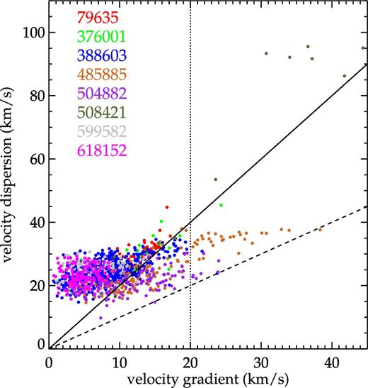
Dependence of gas velocity dispersion (σgas) on velocity gradient (vgrad, equation 1). Points in each individual galaxy are labelled by colour. The solid line refers to σgas = 2vgrad and the dashed line refers to σgas = vgrad. The dotted line denotes the velocity gradient at 20 km s−1. These three different lines represent the three different criteria that we tested to account for beam smearing (Section 2.2.3).
We find that our results do not depend on the particular choice of the beam-smearing cut. All three selection criteria yield consistent results. A flat but elevated distribution of gas velocity dispersion (see more in Section 3.2.1) is shown in all of the three cases. We choose to preserve only the spaxels with σgas > 2 vgrad (those above the black solid line) in the following analysis. Our method here is similar to the simple analytic calculation in Bassett et al. (2014, equation 1).
2.3 Spatial resolution
We compare our sample with high-redshift surveys and local H α luminous galaxies. The data in Lehnert et al. (2013) have FWHM ∼0.6 arcsec and pixel scale 0.25 arcsec corresponding to 5 and 2 kpc at z ∼ 2. The seeing limit of our sample is ∼ 2.5 arcsec and the pixel scale is 0.5 arcsec, which correspond to 2.5 and 0.5 kpc at z ∼ 0.05. Genzel et al. (2017) has FWHM up to 0.2 arcsec corresponding to ∼ 1.5 kpc at z ∼ 0.76–2.65. Green et al. (2014) has spatial resolutions of 1–3 kpc. We reach similar resolutions as Genzel et al. (2011) and Green et al. (2014) and better than Lehnert et al. (2013). All the works above either construct models or use simulations to remove the beam-smearing effect.
3 RESULTS
We investigate the relation between ΣSFR and σgas spaxel by spaxel (locally), and within individual galaxies (globally), to see if star formation drives the velocity dispersion in these local star-forming galaxies.
3.1 The spatial distribution of ΣSFR, vgas and σgas
In Fig. 1, we show the maps of ΣSFR, gas velocity and gas velocity dispersion for each of our eight galaxies. The major axes and galaxy centres are labelled in the images. We see the following.
The ΣSFR maps have various distributions. There are often multiple peaks and rings, and some of the peaks are not at the centre, indicating local structures such as spiral arms, star-forming clumps, etc.
All galaxies show clear velocity gradients indicating rotation.
All galaxies show a gas velocity dispersion peak at the centre.
The distribution of gas velocity dispersion does not always follow the distribution of ΣSFR (i.e. the peaks in σgas do not always correlate with those in ΣSFR). This is self-consistent because regions of intense mechanical or radiative energy injections (e.g. star-forming regions) are over-pressured and compact while overpressurized gas is over a much larger scale.
3.2 The σgas–ΣSFR relation in local and high redshift star-forming galaxies
3.2.1 Local (spaxel-by-spaxel) analysis
After removing the spaxels with high vgrad (keeping those with σgas > 2vgrad), we compare the spatially resolved relation between σgas and ΣSFR in our local galaxies with that in high redshift galaxies (Lehnert et al. 2009) in Fig. 3 . We also insert a zoom-in of our SAMI data with a logarithmic y-axis.
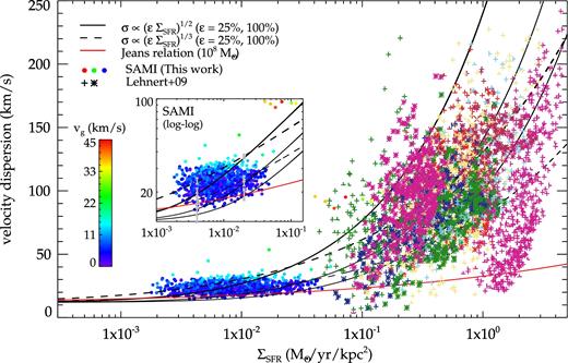
Spatially resolved dependence of σgas on ΣSFR. We remove pixels with vgrad > 0.5σgas to account for beam-smearing effects (see Fig. 2 and Section 2.2). Our eight SAMI galaxies are compared to Lehnert et al. (2009, fig. 12 therein). Each filled circle refers to one spaxel in each galaxy and is colour-coded with the magnitude of velocity gradient (vgrad, equation 1). The crosses and asterisks in different colours refer to the 11 actively star-forming galaxies at z ∼ 2 in Lehnert et al. (2009). The solid black curves show |$\sigma \propto (\epsilon \dot{E})^{1/2}$|, where |$\dot{E}$| is the energy injection due to star formation, and ε is the coupling efficiency of the energy injected into the ISM. The dashed curves show |$\sigma \propto (\epsilon \dot{E})^{1/3}$| assuming that velocity dispersions correspond to energy dissipation due to turbulent motions. The red solid curve shows the velocity dispersion of a 108 M⊙ clump assuming a simple Jeans relation. A zoom-in of our SAMI galaxies with a logarithmic y-axis is also shown here. All of the models have included the typical thermal broadening of H α of 12 km s−1. The error bars in the zoom-in figure show the maximum range of the thermal broadening of 10–15 km s−1. The colour bar on the left shows the magnitude of the velocity gradient (v|$\rm _g$|).
As shown by the filled circles, the velocity dispersion of our local star-forming galaxies is almost constant around 20 km s−1, covering a ΣSFR range of over an order of magnitude. As discussed in Section 2.2.2, SAMI is able to detect σgas below 15 km s−1 for a sufficiently high S/N (here 34); therefore, the cut-off at ∼15 km s−1 represents a physical cut-off. The flat and tight distribution of σgas in our local star-forming galaxies does not present an obvious correlation with ΣSFR. There are some outliers with σgas > 40 km s−1 that may result from a shocked component in 508421 as mentioned in Sections 2.1.2 and 2.2.3.
We also connect the behaviour of the gas in star-forming galaxies from low-z to high-z by superimposing our data on to the results in fig. 12 from Lehnert et al. (2009). The crosses and asterisks in different colours refer to the 13 actively star-forming galaxies at z ∼ 2 in Lehnert et al. (2009). The high-redshift galaxies in Lehnert et al. (2009) show higher velocity dispersion with larger scatter than our local star-forming galaxies. They are also more or less positively correlated with ΣSFR, however, with substantial scatter. This may indicate that star formation feedback plays a more important role in high-redshift star-forming galaxies than in their local counterparts. High-redshift star-forming galaxies, as shown in Genzel et al. (2011, 2014), are mostly irregular and clumpy while local galaxies are stable and rotationally supported, as seen in Fig. 1. Therefore, juvenile high-redshift galaxies could be more easily affected by their intense star formation activity and mature local galaxies could be more sensitive to galactic-scale dynamics like cloud–cloud collisions, galactic shear, self-gravity and MRI than to star formation feedback. We discuss this further in Section 4.
3.2.1.1 Theoretical models for σgas.
The curves in Fig. 3 denote different models proposed by Lehnert et al. (2009) to explain the relation between σgas and ΣSFR.
If the dissipated energy comes from star formation, and star formation induces high pressures, then a simple scaling relation is expected. This is indicated by the solid black curves, in the form |$\sigma \propto (\epsilon \dot{E})^{1/2}$|, where |$\dot{E}$| is the energy injection rate due to star formation, and ε is the coupling efficiency between the injected energy and the ISM. According to Dib et al. (2006), when modelling the ISM with a coupling efficiency of 25 per cent (a conservative value), quiescent galaxies may switch to a starburst mode at ΣSFR = 10−2.5 to 10−2 M⊙ yr−1 kpc−2. The bottom two black solid lines are derived from such models using these two values, showing |$\rm \sigma _{\rm gas} = 100 \Sigma _{\rm SFR}^{1/2}$| and |$\rm \sigma _{\rm gas} = 140 \Sigma _{\rm SFR}^{1/2}$| (σgas is in km s−1, ΣSFR is in M⊙ yr−1 kpc−2, the same below). The third curve at the top shows |$\rm \sigma _{\rm gas} = 240 \Sigma _{\rm SFR}^{1/2}$|, using coupling efficiencies of 100 per cent (an extreme and unrealistic value).
If the energy is dissipated through incompressible turbulence, another scaling relation would be expected. This is shown by the dashed curves in the form of |$\sigma _{\rm gas} \propto (\epsilon \dot{E})^{1/3}$|, where |$\dot{E}$| is the energy dissipated through turbulence. The two black dashed curves show |$\rm \sigma _{\rm gas} = 80 \Sigma _{\rm SFR}^{1/3}$| and |$\rm \sigma _{\rm gas} = 130 \Sigma _{\rm SFR}^{1/3}$|, using coupling efficiencies of 25, 100 per cent, and a primary injection scale of 1 kpc.
If the turbulence is powered by gravity, assuming a simple Jeans relationship between mass and velocity dispersion, Lehnert et al. (2009) derived the relation in the form of σgas ∼ |$M_{J}^{1/4}G^{1/2}\Sigma _{\rm gas}^{1/4}$| = 54 km s−1|$M_{J,9}^{1/4}\Sigma _{\rm SFR}^{0.18}$|, where G is the gravitational constant, Σgas is the gas mass surface density in M⊙ pc−2, MJ, 9 is the Jeans mass in units of 109 M⊙ and ΣSFR is in M⊙ kpc−2 yr−1. The red solid curve shows the velocity dispersion as a function of ΣSFR of a 108 M⊙ giant molecular cloud (GMC). Given the mass of our local star-forming galaxies are similar to the Milky Way, there is not any molecular cloud more massive than 108 M⊙ (Roman-Duval et al. 2010), which means that the red curve represents an upper limit for the velocity dispersion obtained via the Jeans relation proposed by Lehnert et al. (2009)
Due to a characteristic temperature of 104 K (Andrews & Martini 2013), the H α emission line has a typical thermal broadening of ∼ 12 km s−1. In addition, the temperature distribution in an H ii region is not uniform, so we estimate a maximum range of 10–15 km s−1 (Andrews & Martini 2013). Here, in all of the models we include the intrinsic thermal broadening of 12 km s−1, but we also display the maximum range with the error-bars in the zoom-in figure.
None of the models can properly explain our local star-forming galaxies. |$\sigma \propto (\epsilon \dot{E})^{1/2}$| and |$\sigma \propto (\epsilon \dot{E})^{1/3}$| are consistent with some of the spaxels in our SAMI galaxies. However, all of the relations predict lower velocity dispersion than seen in a significant number of spaxels. Most of the data points of our galaxies are significantly above the bottom two black solid lines and the bottom black dashed line, which correspond to a realistic coupling efficiency of 25 per cent (Dib et al. 2006) in the two models. Even if we consider the most extreme (and unrealistic) cases with coupling efficiencies of 100 per cent, as shown by the top black solid line and the top black dashed line, the data points at the lower ΣSFR end cannot be well explained. The same is true with the Jeans instability relation. Even if we assume extreme GMC masses as high as 108 M⊙, it still underestimates the velocity dispersion of our galaxies. Moreover, the error bars in the zoom-in figure indicate that the uncertainty induced by the thermal broadening has minor influence on the distribution of the models. Therefore, simply considering energy injection from star formation, dissipation of incompressible turbulence, or release of gravitational energy alone as the source of velocity dispersion is not enough to explain the distribution of gas velocity dispersion in local star-forming galaxies.
3.2.2 Global (galaxy-averaged) analysis
In Fig. 4 , we look at the global behaviour of the gas in star-forming galaxies. We include the local H α luminous galaxies from Green et al. (2014) as green diamonds, and the z > 1 star-forming galaxies and star-forming clumps with good data quality,2 for comparison. The area used to calculate the ΣSFR of galaxies in Green et al. (2014) are from the radii based on an exponential model fit. Given their various sizes, they span a very large range of ΣSFR. The global ΣSFRs and velocity dispersions of our eight galaxies are listed in Table 2. The global ΣSFRs and velocity dispersions are the flux weighted averages of spaxels within individual galaxies. Only the spaxels with σgas > 2vgrad are considered in the measurement. All these works derive velocity dispersion from the H α emission lines. The grey contour denotes the distribution of local star-forming galaxies with σgas derived from H i (Dib et al. 2006), and we include the intrinsic thermal broadening of 12 km s−1 here. The difference in velocity dispersions between H i and H α comes from the thermal broadening of warm ionized gas at ∼ 104 K.
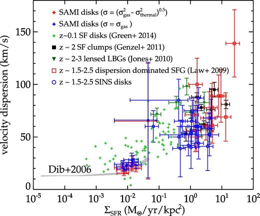
Global dependence of σgas on ΣSFR. Our eight SAMI galaxies compared to local high H α luminosity galaxies from Green et al. (2014) and z > 1 star-forming galaxies and clumps (see Section 3.2.2 for further details). Each blue (red) filled diamond shows one entire galaxy in our sample including (excluding) the contribution from thermal broadening (σthermal ∼ 12 km s−1; Glazebrook 2013). For the measurement of σgas and ΣSFR, see footnotes in Table 2. Green diamonds refer to the H α luminous galaxies in Green et al. (2014). The black filled squares, dark green triangles, red open squares and blue open circles refer to the z > 1 star-forming galaxies and clumps. The grey contour denotes the distribution of local star-forming galaxies with gas velocity dispersion derived from H i (Dib, Bell & Burkert 2006), and we include the intrinsic thermal broadening of 12 km s−1 here.
Comparing our eight SAMI galaxies to the high-redshift galaxies, we see similar behaviour to the spatially resolved data (cf. Fig. 3). When taking the 67 H α luminous galaxies from Green et al. (2014) into account, we find that it can well connect the local and high-redshift galaxies. In Fig. 4, we see that their distribution at the lower ΣSFR end agrees with the distribution of our eight galaxies and the higher ΣSFR end follows the distribution of the high-redshift galaxies as well. The Green et al. (2014) local star-forming galaxies are chosen to have similar properties to the high-redshift galaxies, such as high gas fraction and high H α luminosities (≳ 1042 erg s−1). Note that we calculate the ΣSFR of galaxies in Green et al. (2014) without flux weighting, so the ΣSFR may be underestimated compared to other galaxies.
We measure the Spearman correlation coefficients between gas velocity dispersion and ΣSFR, for three different groups of the three sets of data. The results are listed in Table 3 . Our eight SAMI galaxies together with the Green et al. (2014) H α luminous galaxies show strong correlation between velocity dispersion and ΣSFR (rs = 0.72). When we include the high-z galaxies, the correlations become a bit stronger (rs = 0.76). However, when combining our eight SAMI galaxies with only the high-z galaxies, the correlation becomes moderate (rs = 0.53). Note that the global ΣSFR are flux weighted. Therefore, this result comes from relatively more active star-forming regions, which is not contrary to the conclusion we draw from the spatially resolved analysis in Section 3.2.1. Stellar feedback alone is insufficient to drive the observed σgas, especially at low SFR surface density (Section 3.2.1), while it can become dominant when SFR surface density is high enough (Section 3.2.2).
Spearman correlation coefficient (rs).
| σgas versus ΣSFR | ||
|---|---|---|
| rs | Pc | |
| SAMI + greena | 0.72 | ≪0.01 |
| SAMI + high-zb | 0.53 | ≪0.01 |
| SAMI + greena + high-zb | 0.76 | ≪0.01 |
| σgas versus ΣSFR | ||
|---|---|---|
| rs | Pc | |
| SAMI + greena | 0.72 | ≪0.01 |
| SAMI + high-zb | 0.53 | ≪0.01 |
| SAMI + greena + high-zb | 0.76 | ≪0.01 |
4 DISCUSSION
4.1 Main driver(s) of velocity dispersion
As mentioned in Section 3.2.1, the flat and elevated (compared to the model predictions) distribution of spaxels of our SAMI galaxies shown in Fig. 3 indicates that the star formation feedback is unlikely to dominate the gas velocity dispersion at the scale of ∼ 0.5 × 0.5 kpc2. Thus, additional drivers of turbulence must be acting in these local, low ΣSFR galaxies. As indicated by the flatness of the distribution, such sources need to be common among galaxies and not vary much within galaxies.
The drivers of turbulence can either compress the gas (compression processes) or directly excite solenoidal motions of gas (stirring processes) (Federrath et al. 2016, 2017).
Stellar feedback like stellar winds of OB stars and Wolf–Rayet stars, supernova explosions, as well as accretion processes (such as accretion on to a galaxy) and gravitational contraction are able to compression the gas, and then increase gas velocity dispersion and induce star formation at the same time. Therefore, SFR (or ΣSFR) may not be directly related to gas velocity dispersion. Both SFR (or ΣSFR) and gas velocity dispersion can be affected simultaneously by the same sources (e.g. accretion, gravity, etc.), but to different degree.
Krumholz & Burkhart (2016) proposed that the turbulence in the ISM is driven by gravity rather than stellar feedback. The higher (than expected) velocity dispersion in Fig. 3 may be due to the release of gravitational energy. However, the Krumholz & Burkhart (2016) conclusion comes from the constraint of rapid star-forming, high-velocity dispersion galaxies. Their models do not show any apparent difference at low velocity dispersion. Moreover, they investigate the relation with SFR rather than ΣSFR and on entire galaxies rather than on spatially resolved regions. On the other hand, the Lehnert et al. (2009) models in Fig. 3 reveal that – (i) self-gravity is not sufficient even if the model (red solid curve) adopts an extremely massive the star-forming clump as 108 M⊙, which is too big for local star-forming galaxies; (ii) turbulence can be driven by the bulk motions induced by energy injection from star formation, and then cascade, redistribute and dissipate the energy down to smallest scales. Star formation powers the turbulence of galaxies with high-velocity dispersions in complex ways, but star formation alone is insufficient to explain the gas velocity dispersions in our local star-forming galaxies. Generally, both gravity and star formation can power the turbulence but dominate at different redshifts and/or in different environments.
Stirring processes like galactic shear, MRI and jets/outflows can induce solenoidal motions, i.e. increase the velocity dispersion, but suppress the star formation. Shear is a typical driver of the turbulence in the centres of our galaxy and possibly other galaxies (Krumholz & Kruijssen 2016; Kruijssen 2017; Federrath et al. 2016, 2017). MRI requires a combination of rotation and magnetic fields. Compared to compressive stirring mechanisms, solenoidal stirring processes have less influence on the density distribution (Federrath, Klessen & Schmidt 2008; Federrath et al. 2010). Therefore, solenoidal driving mechanisms reduce the SFR compared to compressive sources of σgas (Federrath & Klessen 2012). Solenoidal drivers (such as MRI and shear) may be able to provide an explanation for the distribution of our SAMI galaxies in Fig. 3: suppressed ΣSFR but relatively higher gas velocity dispersion than expected from star formation feedback.
Note that the velocity modes (solenoidal and compressible) do not grow independently of one another (for a detailed analysis in the case of compressive and solenoidal driving of the turbulence, see Federrath et al. (2010, fig. 14) and Federrath et al. (2011, fig. 3 bottom panel)). However, what we are referring to here when we talk about solenoidal and compressive modes, are the modes in the acceleration field (not the resulting velocity field) that drives the turbulence. A summary of the differences and implications of solenoidally and compressively driven turbulence and their implications for star formation is presented in Federrath et al. (2017) and the main theoretical framework as well as comparison to observations are presented in Federrath & Klessen (2012).
4.2 Caveats
4.2.1 The medium being observed
H α emission traces ionized gas and gives information on the turbulences in H ii regions. We may miss out the tracers showing the star formation feedback and effects of turbulence driven by galaxy dynamics (such as shear) by just analysing the ionized gas (and not including the atomic and molecular phases). Studies such as Stilp et al. (2013) find two component fits are necessary for H i lines in nearby galaxies, and the broad components are mainly related to the star formation intensity, which support the idea of star formation supporting the turbulence and gravitational instability/shear. Here, we are limited to strong emission line data, but we have applied for ALMA time to follow-up a subset of our galaxies to study the velocity dispersion in the cold/molecular gas as well.
4.2.2 Removing the inner regions of the galaxies
In this paper, circumnuclear regions of our galaxies are removed because of the strong influence of beam smearing. However, circumnuclear regions are very interesting and important in order to develop a complete picture of turbulence injection across a galaxy. The influence of the rotation curve could be especially important in circumnuclear regions, providing a strong test of the gravitational shear/instability arguments. The broadest molecular lines are also found in the circumnuclear gas of galaxies suggesting that star formation is playing a crucial role there (e.g. Wilson et al. 2011). Here, we chose to exclude the inner regions, where beam smearing significantly affects our data. Future studies that attempt to correct for beam smearing will be needed to investigate the turbulence in the circumnuclear regions in detail.
4.2.3 Removing the galaxies that show any evidence for shocks
Shock-driven turbulence contains important information about the connection between star formation feedback and turbulence. However, it is difficult to disentangle the contribution of star formation from possible AGN activity to extract actual SFRs accurately from the shock-heated gas. We would likely overestimate SFRs and thus overestimate the effect of star formation feedback. Thus, in a conservative way, we chose not to include any galaxies with signatures of shock-excited emission and focus on purely star-forming galaxies.
4.2.4 Dependence of velocity dispersion on rotational velocity
Fig. 5 shows the dependence of velocity dispersion on rotational velocity. Overall, we see no strong dependence. However, we see some trends of decreasing velocity dispersion with increasing velocity, especially along the major axes (labelled with error bars). The beam-smearing effect would be higher in the centre than the outside. For our galaxies, we have already removed the highly affected spaxels; thus, the circumnuclear regions are removed (Section 4.2.2).
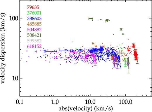
Velocity dispersion as a function of velocity. Spaxels along the major axis are plotted with error bars. Points in each individual galaxy are labelled by colour.
5 CONCLUSION
Random, turbulent motions are important in regulating the star formation in the galaxies, but the energy source of turbulent motions remains unclear. We investigate the random motions of the ionized gas in local star-forming galaxies. After very strict selection to avoid the possible contamination by AGNs, shocks and outflows, we find eight SAMI galaxies satisfying the pure star-forming criteria based on emission line diagnostic diagrams. We minimize the influence of beam smearing by removing the spaxels with σgas < 2 vgrad before further analysis (Fig. 2). The spatially resolved images and high spectral resolution of the SAMI Galaxy Survey shows that, on scales of 0.5 × 0.5 kpc2, turbulence within local star-forming galaxies is not exclusively driven by star formation feedback. The flat but elevated (compared to model predictions) distribution of gas velocity dispersion as a function of ΣSFR (Fig. 3) implies that there must be some additional energy source(s) besides star formation feedback, especially at the low ΣSFR end. Such source(s) need to be common among local star-forming galaxies and do not vary spatially across galaxies. The difference with the high-redshift galaxies and H α luminous galaxies (Figs 3 and 4) indicates that the low SFR in these local galaxies is too weak to explain the random motions of the ionized gas. Juvenile high-redshift galaxies could be more sensitive to their intense star formation activity while mature local galaxies could be more influenced by galactic-scale dynamics like gravity, galactic shear and MRI than by star formation feedback.
Acknowledgements
LZ and YS acknowledge support for this work from the National Natural Science Foundation of China (NSFC grant 11373021) and the Excellent Youth Foundation of the Jiangsu Scientific Committee (grant BK20150014). CF gratefully acknowledges funding provided by the Australian Research Council’s Discovery Projects (grants DP150104329 and DP170100603). Support for AMM is provided by NASA through Hubble Fellowship grant no. HST-HF2-51377 awarded by the Space Telescope Science Institute, which is operated by the Association of Universities for Research in Astronomy, Inc. for NASA, under contract NAS5-26555. We thank R. Genzel, N. Förster Schreiber, M.D. Lehnert and N.P.H. Nesvadba for their support on providing high-z measurements displayed in this work. We thank the anonymous referee for his/her thorough review and highly appreciate the comments and suggestions, which significantly contributed to improving the quality of the publication. MSO acknowledges the funding support from the Australian Research Council through a Future Fellowship (FT140100255). BC acknowledges support from the Australian Research Council’s Future Fellowship (FT120100660) funding scheme. SB acknowledges the funding support from the Australian Research Council through a Future Fellowship (FT140101166). SFS thanks PAPIIT-DGAPA-IA101217 project and CONACYT-IA-180125. We would like to thank the anonymous reviewer for his/her helpful and constructive comments that greatly contributed to improving the final version of the paper.
The SAMI Galaxy Survey is based on observations made at the Anglo–Australian Telescope. The Sydney-AAO Multi-object Integral field spectrograph (SAMI) was developed jointly by the University of Sydney and the Australian Astronomical Observatory. The SAMI input catalogue is based on data taken from the Sloan Digital Sky Survey, the GAMA Survey and the VST ATLAS Survey. The SAMI Galaxy Survey is funded by the Australian Research Council Centre of Excellence for All-sky Astrophysics (CAASTRO), through project number CE110001020, and other participating institutions. The SAMI Galaxy Survey website is http://sami-survey.org/.
Extinction-corrected SDSS DR7 Petrosian mag.
Which includes – (a) z ∼ 2 star-forming clumps (Genzel et al. 2011) as black filled squares; (b) z ∼ 2–3 low mass (∼ 109 M⊙) lensed star-forming galaxies (Jones et al. 2010) as dark green triangles; (c) z ∼ 1.5–3 low mass (∼ 0.3–3 × 10¹⁰ M⊙), compact but well resolved with adaptive optics ‘dispersion dominated’ star-forming galaxies (Law et al. 2009) as red open squares; (d) z ∼ 1.5–2.5 discs from the SINS survey (Cresci et al. 2009; Förster Schreiber et al. 2009) as blue open circles.
REFERENCES
