


Abstract
We investigate the impact of galactic outflow modelling on the formation and evolution of a disc galaxy, by performing a suite of cosmological simulations with zoomed-in initial conditions (ICs) of a Milky Way-sized halo. We verify how sensitive the general properties of the simulated galaxy are to the way in which stellar feedback triggered outflows are implemented, keeping ICs, simulation code and star formation (SF) model all fixed. We present simulations that are based on a version of the gadget3 code where our sub-resolution model is coupled with an advanced implementation of smoothed particle hydrodynamics that ensures a more accurate fluid sampling and an improved description of gas mixing and hydrodynamical instabilities. We quantify the strong interplay between the adopted hydrodynamic scheme and the sub-resolution model describing SF and feedback. We consider four different galactic outflow models, including the one introduced by Dalla Vecchia & Schaye (2012) and a scheme that is inspired by the Springel & Hernquist (2003) model. We find that the sub-resolution prescriptions adopted to generate galactic outflows are the main shaping factor of the stellar disc component at low redshift. The key requirement that a feedback model must have to be successful in producing a disc-dominated galaxy is the ability to regulate the high-redshift SF (responsible for the formation of the bulge component), the cosmological infall of gas from the large-scale environment, and gas fall-back within the galactic radius at low redshift, in order to avoid a too high SF rate at z = 0.
1 INTRODUCTION
The formation of disc galaxies with a limited bulge and a dominant disc component is a challenging task in cosmological simulations of galaxy formation (e.g. Mayer, Governato & Kaufmann 2008; Scannapieco et al. 2012). The astrophysical processes involved in the cosmological formation and evolution of these galaxies span a wide dynamical range of scales, from the ∼parsec (pc) scales typical of star formation (SF) to the ∼Mpc scales where gravitational instabilities drive the evolution of the dark matter (DM) component and the hierarchical assembly of galaxy-sized haloes, passing through the ∼kpc scales where galactic winds distribute the feedback energy from SF processes to the surrounding gas, thereby regulating its accretion and subsequent SF. Sub-resolution models are thus essential to model processes that take place at scales not resolved by cosmological hydrodynamic simulations of galaxy formation, but that affect the evolution on scales that are explicitly resolved. In general, these sub-resolution models resort to a phenomenological description of rather complex processes, through a suitable choice of parameters, that need to be carefully tuned by asking simulations to reproduce basic observational properties of the galaxy population.
Stellar feedback, that triggers galactic outflows, is a crucial component in simulations that want to investigate galaxy formation. It contributes to determine the overall evolution of galaxies (Stinson et al. 2013; Aumer et al. 2013; Marinacci, Pakmor & Springel 2014; Murante et al. 2015, M15 hereafter), to shape their morphology (Crain et al. 2015; Hayward & Hopkins 2017), to set their sizes and properties (Vogelsberger et al. 2014; Schaye et al. 2015). Additionally, stellar feedback driven winds are expected to expel low angular momentum gas at high redshift from the innermost galaxy regions and to foster its following fall-back, once further angular momentum has been gained from halo gas (Brook et al. 2012; Übler et al. 2014; Teklu et al. 2015; Genel et al. 2015). Galactic outflows contribute to the continuous interaction between galaxies and their surrounding medium, and allow for the interplay between stars and different components of the interstellar medium (ISM). Using non-cosmological simulations of isolated galaxies, Gatto et al. (2017) recently pointed out that strongly star-forming regions in galactic discs are indeed able to launch supernova (SN)-driven outflows and to promote the development of a hot volume-filling phase. They also noted a positive correlation between outflow efficiency, i.e. the mass loading factor, and the hot gas volume-filling fraction. Moreover, Su et al. (2016) have recently shown that stellar feedback is the primary component in determining the star formation rate (SFR) and the ISM structure, and that microphysical diffusion processes and magnetic fields only play a supporting role.
Despite the general consensus on the need of stellar feedback to form spiral galaxies that are not too much centrally concentrated and have a dominant disc component, it is still unclear which are the sub-resolution models able to capture an effective description of feedback energy injection, and how to select the best ones among them. Different stellar feedback prescriptions are succeeding in promoting the formation of disc galaxies and a variety of approaches have been so far proposed to numerically describe galactic outflows (see M15, and references therein).
For instance, Übler et al. (2014) contrasted galaxy formation models that adopt different stellar feedback prescriptions: a weak feedback version (Oser et al. 2010) that promotes spheroid formation, and a strong feedback scheme (Aumer et al. 2013) that favours disc formation. They also compared the predicted mass assembly histories for systems with different virial masses. Agertz & Kravtsov (2016) investigated the effect of different SF and stellar feedback efficiencies on the evolution of a set of properties of a late-type galaxy: they highlighted that morphology, angular momentum, baryon fraction, and surface density profiles are sensitively affected by the analysed parameters. A grasp on the comparison between distinct galactic outflow models would reveal vital information on the effects and consequences of diverse schemes, especially when these are implemented within the same prescriptions for SF and cooling, in the same code.
The Aquila comparison project (Scannapieco et al. 2012) brought out the crucial importance of the description of the ISM below the resolution achievable in simulations and showed how different schemes for SF and stellar feedback lead to the formation of galaxies having rather different properties. Besides the importance of the sub-resolution prescriptions, Scannapieco et al. (2012) pointed out that a non-negligible role in determining the simulation results is also played by the choice of the underlying hydrodynamical scheme, either Eulerian or Lagrangian smoothed particle hydrodynamics (SPH).
Great effort has been therefore devoted to improving numerical techniques and enhancing hydrodynamical solvers. Advanced SPH schemes have been proposed: modern versions of SPH adopt more accurate kernel functions, include time-step limiters and introduce correction terms, such as artificial conduction (AC) and viscosity (AV), in order to properly deal with fluid mixing, to accurately describe the spread of entropy and to follow hydrodynamical instabilities (Price 2008; Saitoh & Makino 2009; Cullen & Dehnen 2010; Dehnen & Aly 2012; Durier & Dalla Vecchia 2012; Pakmor et al. 2012; Price 2012; Valdarnini 2012; Beck et al. 2016). Other enhanced SPH flavours adopt a pressure–entropy formulation, in addition (Saitoh & Makino 2013; Hopkins 2013; Schaller et al. 2015).
In this paper, we will use the version of SPH presented by Beck et al. (2016) that has been implemented in the developer version of the gadget3 code (Springel 2005). This implementation of the SPH has been applied to simulations of galaxy clusters by Rasia et al. (2015), who analysed the cool-core structure of clusters (see also Sembolini et al. 2016a,b; Biffi & Valdarnini 2015). Interestingly, Schaller et al. (2015) analysed the influence of the hydrodynamic solver on a subset of the Eagle simulations. They showed that their improved hydrodynamic scheme does not affect galaxy masses, sizes, and SFRs in all haloes, but the most massive ones; moreover, they highlighted that the higher the resolution is, the more responsive to the accuracy of the hydrodynamic scheme simulation outcomes are expected to be.
The analysis that we present in this paper has been carried out with two main goals. First, the improved SPH implementation by Beck et al. (2016) has been introduced into the TreePM+SPH code gadget3 that we use to perform simulations of galaxy formation. Such an implementation has shown to be able to alleviate a number of problems that historically affect ‘traditional’ SPH flavours, e.g. the spurious loss of angular momentum caused by the AV in shear flows, and the presence of a numerical surface tension force that dumps important hydrodynamical instabilities such as the Kelvin–Helmholtz one. We now want to test the interplay between this new SPH implementation in cosmological simulations of galaxy formation, and our adopted sub-resolution model, named MUPPI (MUlti Phase Particle Integrator), for SF and stellar feedback (Murante et al. 2010, M10 hereafter; M15).
Secondly, we explore a different implementation of feedback models within the MUPPI scheme to highlight the variation in the final results that we obtain by modifying only the description of galactic outflows. We implement and test three different models for the production of galactic outflows, besides the standard one already used by M15. One of these models, that was introduced by Dalla Vecchia & Schaye (2012), is adapted to MUPPI. Another one is similar in spirit to the galactic outflow model originally introduced by Springel & Hernquist (2003), again fitted for MUPPI. The third one is a variation over our standard galactic outflow prescription.
The main questions that we want to address in this paper can be summarized as follows: how much are results of a sub-grid scheme affected by the hydrodynamic solver? How sensitive are the properties of a simulated galaxy when different galactic outflow models are implemented within the same SF model? What are the requirements for a galactic outflow model to lead to the formation of a late-type galaxy with a limited bulge and a dominant disc component?
In Section 2, we describe the code on which the simulations are based: the main modifications introduced by the new hydrodynamical scheme are highlighted (Section 2.1) and the main features of the MUPPI sub-grid model are reviewed (Section 2.2). In Sections 2.3 and 2.4, we provide the description of the coupling of the improved hydrodynamic scheme with the MUPPI model. In Section 3, we introduce the different galactic outflow models that we implemented, in order to investigate and compare their key features when included in MUPPI. In Section 4, the suite of simulations is described. In Section 5, we present and discuss results from cosmological simulations that lead to the formation of disc galaxies, while we draw our main conclusions in Section 6.
2 NUMERICAL MODELS
In this paper, we use a version of the TreePM+SPH gadget3 code, a non-public evolution of the gadget2 code (Springel 2005). In this version of the code, the standard flavour of SPH has been improved by the implementation of hydrodynamics presented in Beck et al. (2016). Furthermore, the code includes the description of a multiphase ISM and the resulting SF model as described in M10 and M15. In this paper, we present for the first time simulations that are based on a version of gadget3 where our SF model is interfaced with the improved implementation of SPH. We describe in this section the relevant aspects of both SPH and SF implementations.
2.1 The improved SPH scheme
Besides the new kernel function, the most important improvements in this new formulation of SPH mainly consist in an advanced treatment of AV and AC.
The inclusion of the AV correction (Cullen & Dehnen 2010; Beck et al. 2016) allows us to suppress AV far from shocks and where unwanted. New second-order estimates for velocity gradients and curls are crucial to this purpose: improved computations of the Balsara switch (Balsara 1995) and of factors that reveal the presence of a shock control the action of AV, by removing it in purely shear flows, and by limiting its effect where the relative motion of gas particles appears convergent because of vorticity or rotation effects, as e.g. in Keplerian flows.
Moreover, in this enhanced implementation a time-step limiting particle wake-up scheme (see Beck et al. 2016, and references therein for a thorough description) has been adopted: it alleviates high discrepancies in the size of time-steps among nearby particles. Indeed, the code integrates quantities of different particles on an individual particle time-step basis: single time-steps are computed according to hydrodynamical properties of particles. Then, at a given time-step, some active particles have their physical properties updated, while other particles with longer time-step are inactive and will be considered only for later integrations. However, inactive particles in underdense regions may not be able to realize an abrupt variation of entropy or velocity of a nearby active particle, and to act accordingly. As a spurious net result, inactive particles are prone to gathering and clumping in regions where they remain almost fixed. The wake-up scheme acts in the following way: by comparing the signal velocity1|$v_{\rm ij}^{\rm sign}$| between particles i and its neighbour j to the maximum signal velocity of j and any possible contributing particle within its smoothing length (i.e. |$v_{\rm j}^{\rm sign}$|), an inactive neighbouring particle can be promoted to be active if |$v_{\rm ij}^{\rm sign} > f_{\rm w} v_{\rm j}^{\rm sign}$|, where fw = 3 has been adopted from hydrodynamical tests (Beck et al. 2016). In this way, time-steps of some particles that were inactive are adapted according to the local signal velocity |$v_{\rm j}^{\rm sign}$| and just woken-up particles are then taken into account in the current time-step.
2.2 Star formation and feedback sub-grid model: MUPPI
The sub-grid MUPPI model (see M10, M15) represents a multiphase ISM and accounts for SF and stellar feedback, both in thermal and kinetic forms. A multiphase particle is the constitutive element of the model: it is made up of a hot and a cold gas components in pressure equilibrium, plus a virtual stellar component. A set of ordinary differential equations describes mass and energy flows between the different components.
where P0 is the pressure of the ISM at which fmol = 0.5. According to this prescription, the hydrodynamic pressure of the gas particle is used as the ISM pressure P entering in the phenomenological relation above. Furthermore, a fraction of the star-forming gas is restored into the hot phase.
exceeds a randomly generated number in the interval [0,1]. In equation (7), M is the total initial mass of a gas particle, and ΔM* is the mass of the multiphase star-forming particle that has been converted into stars in a time-step. Each star particle is spawned with mass M* = M/N*, where N* is the number of stellar generations, i.e. the number of star particles generated by each gas particle (we adopt N* = 4; see also M10, Tornatore et al. 2007). Sources of energy that counterbalance the cooling process are: energy directly injected into the ambient ISM by SN explosions (a fraction ffb, local of ESN, the energy provided by each SN), energy provided by thermal feedback from dying massive stars belonging to neighbouring star-forming particles (ffb,out × ESN) and the hydrodynamical source term which accounts for shocks and heating or cooling due to compression or expansion of the gas particle.
A gas particle exits its multiphase stage whenever its density drops below 0.2ρthresh or after a time interval tclock that is chosen to be proportional to the dynamical time tdyn. When a gas particle exits a multiphase stage, it has a probability Pkin of being ‘kicked’ and to become a wind particle for a time interval twind. Both Pkin and twind are free parameters of the outflow model. This scheme relies on the physical idea that stellar winds are powered by type-II SN explosions, once the molecular cloud out of which stars formed has been destroyed. Wind particles are decoupled from the surrounding medium for the aformentioned temporal interval twind. During this time, they receive kinetic energy from neighbouring star-forming gas particles, as described below. None the less, the wind stage can be concluded before twind if the particle density drops below a chosen threshold, 0.3ρthresh.
Kinetic feedback is implemented so that each star-forming particle can provide ffb, kin × ESN as feedback energy. This amount of energy is distributed to wind particles lying inside both the cone and the smoothing length of the star-forming particle, and the delivering mechanism is the same as the thermal scheme. Thus, outflowing energy is modelled so as to leave the star-forming particle through the least-resistance direction (Monaco 2004). Note that only gas particles that were selected to become wind particles are allowed to receive kinetic energy (see Fig. 1).

Cartoon depicting the original galactic outflow model implemented in MUPPI: each star-forming particle provides kinetic feedback energy to neighbour wind particles that are located within a cone of a given opening angle (the purple arrow highlights θ, the half-opening angle). The axis of the cone is aligned as minus the density gradient of the energy donor particle. Energy contributions are weighted according to the distance between wind particles and the axis of the cone.
If there are no particles in the cone, the total amount of thermal energy is given to the particle nearest to the axis (M10, M15). This does not happen with the kinetic energy; in this case, if no eligible wind particle can receive it, the energy is not assigned.
All our simulations include the metallicity-dependent cooling as illustrated by Wiersma, Schaye & Smith (2009), and self-consistently describe chemical evolution according to the model originally introduced by Tornatore et al. (2007), to which we refer for a thorough description. The effect of a uniform time-dependent ionizing cosmic background is also included following Haardt & Madau (2001). Star particles are treated as simple stellar populations with a Kroupa, Tout & Gilmore (1993) initial mass function (IMF) in the mass range [0.1, 100] M⊙. Mass-dependent stellar lifetimes are computed according to Padovani & Matteucci (1993). We account for the contribution of different sources to the production of metals, namely SNIa, SNII, and asymptotic giant branch (AGB) stars. We trace the contribution to enrichment of 15 elements (H, He, C, N, O, Ne, Na, Mg, Al, Si, S, Ar, Ca, Fe, and Ni), each atomic species providing its own contribution to the cooling rate.
2.3 Coupling MUPPI with the improved SPH
An important point in combining the MUPPI SF model and the SPH scheme in which an AC term is included concerns the effect of AC on the thermal structure of the ISM. In fact, we should remind that AC is artificial and introduced as a switch in the energy equation to overcome intrinsic limitations of standard SPH. It does not describe a physical process involving thermal conduction. Therefore, we want to suppress, or turn-off, AC in all the unwanted situations (as described below). One of these situations concerns the description of the thermal structure of the ISM, as provided by a sub-resolution model.
In this context, we remind that our sub-resolution MUPPI model does not rely upon an effective equation of state to describe the ISM, thus we do not impose the pressure of multiphase particles to be a function of the density by adopting a polytropic equation for P(ρ), as e.g. in Springel & Hernquist (2003), and Schaye & Dalla Vecchia (2008).
Within our MUPPI model, each multiphase particle samples a portion of the ISM separately. During the multiphase stage of a particle, external properties as density and pressure can change. The hot phase of the particle can also receive energy from neighbouring star-forming particles, and from SF occurring inside the particle itself. As a consequence, particles’ average temperature can significantly change during the multiphase stage. Since the beginning of the multiphase stage is not synchronized among neighbouring particles, they can be in different evolutionary stages and have different thermodynamical properties.
This is shown in Fig. 2, where we analyse the mass distribution in the density–temperature phase diagram of all gas particles (within the entire Lagrangian region) for a simulation of ours (AqC5-newH; see Section 4 for a description of the simulations used in this work) at redshift z = 0: multiphase particles (whose mass distribution is shown by contours) mainly scatter across a cloud that spans three orders of magnitude in density and almost four in temperature. The temperature plotted in Fig. 2 is, for multiphase particles, the mass-weighted average of the (fixed) temperature of the cold and the hot phases. SPH temperature is considered for single-phase particles and the plotted density is the SPH estimate for all particles. Colours in Fig. 2 encode the gas mass per density–temperature bin.

Phase diagram of all the gas particles (within the entire Lagrangian region) of the AqC5-newH simulation (see Table 1). Contours describe the mass distribution of multiphase particles. The phase diagram is shown at redshift z = 0. Colours encode the gas mass per density–temperature bin (colour scale on the right). Colours of contours are encoded as shown in the bottom colour scale. Bin size is independent for the two distributions, in order to better display the region where they overlap.
Clearly, such a spread would not appear if multiphase particles obeyed an effective equation of state. It is a consequence of the fact that MUPPI does not use a solution of the equations describing the ISM obtained under an equilibrium hypothesis, as e.g. in Springel & Hernquist (2003). Instead we follow the dynamical evolution of the ISM, whose average energy depends on its past history and on the age of the sampled ISM portion. This is the reason why two neighbouring multiphase particles, having the same density, can have quite different internal energies. Note that, in the most active regions of the galaxy, the energy balance of the gas is dominated by the ISM (sub-grid) physics, mainly via thermal feedback. The use of AC among multiphase particles would smear their properties independently of the evolution of the ISM they sample. Thus, AC must not be used when the gas particles are multiphase.
When gas particles exit their multiphase stage in MUPPI, they inherit a mean temperature that has memory of the past multiphase stage. AC between former multiphase particles and surrounding neighbours would smear local properties of the galaxy over wide regions, without preserving the peculiar thermal structure of the galaxy system that the sub-resolution model aims to account for. This is another situation where AC is clearly unwanted.
Finally, wind particles must also be excluded from AC, since we treat them as hydrodynamically decoupled from the rest of the gas. We note that, when they re-couple, there can be a significant difference in internal energy with the medium where they end up.
2.4 A new switch for AC
Therefore, we implemented a prescription that allows AC to be active only when well-defined conditions on the physical properties of the considered particles are met:
AC is switched off for both multiphase particles and wind particles as soon as they enter the wind stage.
Multiphase particles that exit their multiphase stage are not allowed to artificially conduct.
All the non-multiphase particles with AC off (therefore, former multiphase particles and wind particles, too) are allowed to artificially conduct again whenever their temperature differs by 20 per cent at most from the mass-weighted temperature of neighbouring particles.
The physical motivation behind this switch is the following. Multiphase particles have their AC switched off, the hydrodynamics being not able to consistently describe physical processes at the unresolved scales that these particles capture. As soon as a multiphase particle exits its multiphase stage, it will retain physical properties close to the ones it had in advance for some time. For this reason, past multiphase particles keep the AC switched off. When the particle, not sampling anymore the ISM, reaches thermal equilibrium with its surrounding environment, it is allowed to artificially conduct again. We checked the dependence of our results on the exact value of the aformentioned percentage (20 per cent): we found that the precise temperature range within which a particle is allowed to conduct again (i.e. [0.8, 1.2] in our default case) has not a crucial impact on the evolution of the gas, as long as it is narrow enough.
3 IMPLEMENTATION OF GALACTIC OUTFLOW MODELS
The M15 original kinetic stellar feedback implemented in MUPPI successfully produced the massive outflows required to avoid excessive SF and resulted in a lower central mass concentration of the simulated galaxies (M15, Barai et al. 2015). This stellar feedback algorithm produces realistic galactic winds, in terms of wind velocities and mass loading factor (Barai et al. 2015).
We consider here three further numerical implementations of galactic outflows: the first one (FB1 hereafter; Section 3.1) is based on the scheme originally proposed by Dalla Vecchia & Schaye (2012), the second one (FB2 hereafter; Section 3.2) is a modified version of the M15 original kinetic stellar feedback in MUPPI, where particles that are eligible to produce galactic outflows are selected according to a different prescription. The third one (FB3 hereafter; Section 3.3) is a new and distinct model, where the mass loading factor is directly imposed. This third scheme is similar in spirit to that proposed by Springel & Hernquist (2003), adapted to our ISM model.
Our main aim in introducing these three additional schemes is to verify how sensitive the general properties of the simulated galaxy are to the way in which outflows are modelled, while keeping initial conditions (ICs), simulation code, and SF model all fixed. Moreover, we want to investigate how two popular outflow models, namely those by Dalla Vecchia & Schaye (2012) and Springel & Hernquist (2003), perform when implemented within MUPPI.
3.1 FB1: Dalla Vecchia & Schaye model
The model proposed by Dalla Vecchia & Schaye (2012) assumes that thermal energy released by SN explosions is injected in the surrounding medium using a selection criterion: to guarantee the effectiveness of the feedback, the gas particles that experience feedback have to be heated up to a threshold temperature. Such a temperature increase, ΔT, ensures that the cooling time of a heated particle is longer than its sound-crossing time, so that heated gas is uplifted before it radiates all its energy. It is worth noting that stellar feedback is actually implemented as a thermal feedback in this model, since gas particles are heated as a result of the energy provided by type-II SNe, but the effective outcome is a galactic wind, because thermal energy is converted into momentum and hence outflows originate.
The temperature increase ΔTi, or equivalently the temperature at which the gas particle is heated when it experiences feedback, is a free parameter of the model. Dalla Vecchia & Schaye (2012) choose ΔT = 107.5 K as their fiducial temperature increase and found no significative dependence among the values explored, provided that they are above a given threshold that depends on mass resolution and that ensures Bremsstrahlung to dominate the radiative cooling. They also found that cooling losses make their feedback scheme inefficient for gas density above a critical threshold, this floor mainly depending on the temperature threshold described above, on the number of neighbouring particles and on the average (initial) mass of the gas particles. Moreover, when this feedback scheme is adopted in cosmological simulations (Schaye et al. 2015; Crain et al. 2015), a 3 × 10⁷ Myr delay between SF and the release of feedback energy is adopted. Since star particles are expected to move away from the dense regions where they formed, such a time delay helps in delivering energy to gas having lower densities and thus lower radiative losses.
In our implementation of this model, we choose ΔT = 107.5 K as the minimum allowed temperature increase. Then, we account for the presence of gas particles whose density is higher than the maximum density for which this feedback model is expected to be effective (see discussion above), by computing the temperature increase that is needed to guarantee effectiveness. We indeed prefer to adopt a temperature threshold (ΔTi) that varies3 as a function of the gas density (ρi) instead of introducing a delay as a further free parameter. Therefore, we calculate the temperature that each eligible particle has to reach in order to make the feedback effective (from equation 17 of Dalla Vecchia & Schaye 2012), by taking into account the number of neighbour particles that our kernel function adopts, the average (initial) mass of gas particles and a ratio tc/ts = 25 between the cooling and the sound crossing time. After carrying out extensive tests, we found that this value is required to have a feedback that is effective in producing a realistic disc galaxy. The difference with respect to that adopted by Dalla Vecchia & Schaye (2012), tc/ts = 10, should not surprise given that the same outflow model is here applied on a completely different sub-resolution model for the ISM and SF. Hence, in our implementation, the temperature jump of gas particles receiving energy is set to max [ΔT = 107.5 K, ΔTi].
where Z⊙ = 0.0127. Here, nH,0 = 0.67 cm−3, nZ = 0.87, and nn = 0.87 are free parameters of the model. The above analytical expression foretells a ffb,kin that ranges between a high-redshift |$f_{\rm fb, kin}^{\rm \,max}$| and a low-redshift |$f_{\rm fb, kin}^{\rm \,min}$|. The simulation AqC5-FB1 adopts equation (11), keeping both the aforementioned free parameters and |$f_{\rm fb, kin}^{\rm \,max}=3.0$| and |$f_{\rm fb, kin}^{\rm \,min}=0.3$|, as suggested in Schaye et al. (2015, see also Appendix B for further details).
Note that, following the original scheme by Dalla Vecchia & Schaye (2012), we deliver the whole amount of SNII energy when a star is spawned; we do not use the continuous SFR provided by our SF model. The reason for this choice will be detailed in Section 5.3.1. We verified that, in our implementation, the stochastic sampling of the SNII deposited energy is accurate to within few per cent, the ratio between the (cumulative) injected and expected SN feedback energy being <4 per cent for all the simulations that adopt this galactic outflow model (including the lower resolution ones discussed in Appendix B).
3.2 FB2: modified MUPPI kinetic feedback
In this model, we revised the kinetic stellar feedback scheme presented in M15. Our original galactic outflow model was designed in order to produce outflows that are perpendicular to the forming disc, along the least-resistance direction. This is obtained by considering as eligible to receive energy only those wind particles lying in a cone centred on each star-forming particle. Moreover, the original model required the presence of a sufficient amount of gas mass to be accelerated and produce an outflow; otherwise, the kinetic energy is considered to be lost. This may happen if no wind particles are present inside the cone.
Using such a scheme the chosen direction of least resistance is that of the star-forming particle that gives energy to the wind one. However, also due to our choice of a new kernel, that adopts a larger number of neighbours, the least-resistance direction of the wind particle could be different from that of the star-forming one. For this reason, we adopted a new scheme in which the least-resistance direction is that of the wind particle receiving energy.
For this reason, each star-forming particle spreads its available amount of kinetic energy, Ekin = ffb,kin × ESN, among all wind particles within the smoothing length, with kernel-weighted contributions (see below). Fig. 3 illustrates this scheme: a wind particle gathers energy from all star-forming particles of which it is a neighbour. The kinetic energy of the receiving particle is then updated, the wind particle being kicked in the direction of minus its own density gradient. Thus, at variance with the original galactic outflow model, star-forming particles give energy isotropically and not within a cone. In this way, density gradients of star-forming particles are not used to give directionality to the outflows. Particles receiving energy use it to increase their velocity along their least-resistance path. Energy contributions are weighted according to the distance that separates each wind particle that gathers energy and the considered energy donor star-forming particle. We note that this is at variance with the original galactic outflow model, where the distance between selected wind particles and the axis of the cone is considered, instead of the radial particle pair separation.

Cartoon showing the FB2 galactic outflow model implemented within the MUPPI algorithm. At variance with the original implementation, a star-forming particle provides its feedback energy to all the wind particles that are located within the smoothing sphere. Each wind particle is kicked in the direction of minus its own density gradient. Energy contributions are weighted according to the distance between wind particles and the energy donor star-forming particle.
3.3 FB3: fixing the mass loading factor
This model provides a new version of the original MUPPI kinetic feedback model, that we described above, where we directly impose the mass load, instead of using as a free parameter the probability Pkin to promote gas particles to become wind particles.
We aim at implementing a model similar to that of Springel & Hernquist (2003). In their model equilibrium is considered to be always achieved: therefore, ISM properties and consequent SFR are evaluated in an instantaneous manner for each multiphase star-forming particle. Each star-forming particle has then a probability to become a wind particle.
In our model, a multiphase particle remains in its multiphase stage for a given time: this time is related to the dynamical time of the cold phase and computed when a sufficient amount of cold gas has been produced. Our model also takes into account the energy contribution from surrounding SN explosions, i.e. neighbouring star-forming particles contribute to the energy budget of each multiphase particle.
We estimate ISM properties averaged over the lifetime that each multiphase particle spends in its multiphase stage. We then use these properties to determine the probability for each multiphase particle of receiving kinetic energy and thus becoming a wind particle once it exits its multiphase stage. For this reason, we have to sum the energy contributions from SN explosions provided by star-forming particles over the multiphase stage of each gas particle receiving the energy. Moreover, we also have to estimate the mass of gas that goes in outflow, and to compute time-averaged quantities.
In what follows, we always use the index i when referring to star-forming, energy-giving particles, and the index j for particles that receive that energy.
In our FB3 model, particles that receive energy are the multiphase neighbours of multiphase star-forming particles within their entire smoothing sphere. Each of these multiphase particles collects energy from all its neighbouring multiphase star-forming particles and stores it during its entire multiphase stage.
In this way, each multiphase particle j samples the SFR of its neighbours; this SFR is associated to the mass of the star-forming particle as far as the estimate of the mass loss is concerned, not to that of the receivers. At the same time, each multiphase particle collects the SNII energy output from the same star-forming particles. Note that each star-forming particle gives its entire energy budget to all the receivers. A particle ending its multiphase stage receives feedback energy and is uploaded into an outflow with its probability pj. The kinetic energy of the receiving multiphase particle is therefore updated, the particle being kicked in the direction of minus its own density gradient. Particles that experience feedback are hydrodynamically decoupled (for a time interval twind = 15 Myr) from the surrounding medium as soon as they gain feedback energy.
We verified that the stochastic sampling correctly represents the desired mass loading factor and energy deposition to within 5 per cent in the considered cases. This figure can slightly vary with the parameters of the model, as in our FB1 scheme; as for FB1 model, resolution leaves the accuracy of the stochastic sampling almost unaffected.
where εSNII is the thermal energy per unit stellar mass released by type-II SNe (that only depends on the chosen IMF). For this reason, our model is similar to that of Springel & Hernquist (2003). The important change is that SNII energy and SFRs are collected during the life of the portion of the ISM that is sampled, taking into account the fact that changes in the local hydrodynamics (e.g. mergers, shocks, and pressure waves) can influence these values.
Also in this model, thermal energy is still distributed according to the original MUPPI scheme.
4 THE SET OF SIMULATIONS
We performed cosmological simulations with zoomed-in ICs of an isolated halo of mass Mhalo, DM ≃ 2 × 10¹² M⊙, expected to host a disc galaxy resembling the Milky Way (MW), also because of its quiet low-redshift merging history. The ICs used in this work have been first introduced by Springel et al. (2008) and then used, among others, in the Aquila comparison project (Scannapieco et al. 2012). We refer to these ICs as AqC in the paper. These ICs are available at different resolutions: here we consider an intermediate-resolution case with a Plummer-equivalent softening length for the gravitational interaction of 325 h−1 pc (AqC5), and a lower resolution version (AqC6, with a maximum physical gravitational softening of 650 h−1 pc). Further details related to these ICs are given by M15. The cosmological model is unchanged, thus we use a Λcold dark matter cosmology, with Ωm = 0.25, ΩΛ = 0.75, Ωbaryon = 0.04, and H0 = 73 km s−1 Mpc−1.
Even if the mass of the AqC halo is similar to that of the MW, no attempts to mimic the accretion history of its dynamical environment were made. Thus, our simulations should not be taken as a model of our Galaxy.
We list the series of simulations that we ran in order to quantify the impact of the new hydrodynamical scheme in Table 1. Each simulation was given a name: the identifying convention encodes the resolution of the simulation (AqC5 or AqC6) and the adopted hydrodynamical scheme, where newH refers to the improved SPH implementation (Beck et al. 2016) and oldH indicates the standard SPH scheme. Mass resolutions (for both gas and DM particles) and gravitational softenings are also provided in Table 1. All these simulations adopt the original M15 galactic outflow model.
Name and details of the simulations used in order to quantify the impact of the hydrodynamical scheme. Column 1: label of the run. Column 2: mass of DM particles. Column 3: initial mass of gas particles. Column 4: Plummer-equivalent softening length of the gravitational interaction. Column 5: hydrodynamic scheme. Column 6: galactic outflow model.
| Simulation | MDM (h−1 M⊙) | Mgas (h−1 M⊙) | εPl (h−1 kpc) | Hydro scheme | Stellar feedback |
|---|---|---|---|---|---|
| AqC5-newH | 1.6 × 10⁶ | 3.0 × 10⁵ | 0.325 | New | Originala |
| AqC5-oldH | 1.6 × 10⁶ | 3.0 × 10⁵ | 0.325 | Old | Original |
| AqC6-newH | 1.3 × 10⁷ | 4.8 × 10⁶ | 0.650 | New | Original |
| AqC6-oldH | 1.3 × 10⁷ | 4.8 × 10⁶ | 0.650 | Old | Original |
Note.aMurante et al. (2015).
We ran simulations AqC5-newH and AqC6-newH adopting the advanced SPH implementation and using the values of the relevant parameters of the MUPPI model as listed in Table 2 (first and third rows).
Relevant parameters of the sub-resolution model. Column 1: label of the run. Column 2: temperature of the cold phase. Column 3: pressure at which the molecular fraction is fmol = 0.5. Column 4: half-opening angle of the cone, in degrees. Column 5: maximum lifetime of a wind particle (see also M15). Column 6: duration of a multiphase stage in dynamical times. Column 7: number density threshold for multiphase particles. Column 8: gas particle's probability of becoming a wind particle. Columns 9 and 10: thermal and kinetic SN feedback energy efficiency, respectively. Column 11: fraction of SN energy directly injected into the hot phase of the ISM. Column 12: evaporation fraction. Column 13: SF efficiency, as a fraction of the molecular gas.
| Simulation | Tc (K) | P0 (kB K cm−3) | θ (°) | twind (Myr) | tclock/tdyn | nthresh (cm−3) | Pkin | ffb,out | ffb,kin | ffb,local | fev | f⋆ |
|---|---|---|---|---|---|---|---|---|---|---|---|---|
| AqC5-newH | 300 | 2 × 10⁴ | 30 | 20−tclock | 1 | 0.01 | 0.05 | 0.2 | 0.7 | 0.02 | 0.1 | 0.02 |
| AqC5-oldH | 300 | 2 × 10⁴ | 60 | 30−tclock | 1 | 0.01 | 0.03 | 0.2 | 0.5 | 0.02 | 0.1 | 0.02 |
| AqC6-newH | 300 | 2 × 10⁴ | 30 | 20−tclock | 1 | 0.01 | 0.03 | 0.2 | 0.8 | 0.02 | 0.1 | 0.02 |
| AqC6-oldH | 300 | 2 × 10⁴ | 60 | 30−tclock | 1 | 0.01 | 0.03 | 0.2 | 0.5 | 0.02 | 0.1 | 0.02 |
AqC5-oldH and AqC6-oldH are the reference simulations with the old hydrodynamical scheme; these simulations marginally differ from the runs that have been presented and described by M15, as described below. Here, we adopt sets of stellar yields that are newer with respect to those used by M15; they are taken from Karakas (2010) for AGB stars, from Thielemann et al. (2003) and Chieffi & Limongi (2004) for type-Ia and type-II SNe, respectively. After this change, the parameter ffb, kin describing the fraction of SN energy directly injected into the ISM had to be slightly fine-tuned again (from 0.6 to 0.5, see Table 2). Such a change modifies only barely the outcome of the original simulations. All the parameters of the sub-resolution model that have been chosen to carry out AqC5-oldH and AqC6-oldH simulations are provided in Table 2 (second and fourth rows).
Table 3 lists the simulations that we carried out in order to investigate the effect of wind modelling on final properties of the simulated disc galaxy. In this table, we summarize the hydrodynamical scheme adopted and the type of galactic outflow model implemented within the MUPPI sub-resolution prescriptions for cooling and SF.
Name and main features of the simulations performed in order to investigate the effect of the adopted galactic outflow model on final properties of the simulated galaxy. Column 1: label of the run. Column 2: hydrodynamic scheme. Column 3: galactic outflow model (see Section 3 for details). All these runs adopt the softening length and masses of DM and gas particles of the simulation AqC5-newH.
| Simulation | Hydro scheme | Stellar feedback |
|---|---|---|
| AqC5-FB1 | New | First outflow modela (3.1) |
| AqC5-FB2 | New | Second new outflow model (3.2) |
| AqC5-FB3 | New | Third new outflow model (3.3) |
| Simulation | Hydro scheme | Stellar feedback |
|---|---|---|
| AqC5-FB1 | New | First outflow modela (3.1) |
| AqC5-FB2 | New | Second new outflow model (3.2) |
| AqC5-FB3 | New | Third new outflow model (3.3) |
Note.aDalla Vecchia & Schaye (2012).
Simulations AqC5-FB1, AqC5-FB2, and AqC5-FB3 all adopt the new hydrodynamical scheme and all have the same gravitational softening and mass resolutions of AqC5-newH. We will compare these simulations to AqC5-newH, that has been performed with the M15 original outflow model, in order to quantify the variation in the final results when modifying the model of stellar feedback.
5 RESULTS
In this section, we present results from the simulations listed in Section 4, that led to the formation of disc galaxies. After discussing the relevance of introducing a switch to suppress AC in star-forming gas particles (Section 5.1), we show the properties of two disc galaxies simulated by adopting the new and the old hydrodynamic schemes, respectively, and we focus on the differences between the two SPH implementations (Section 5.2). In Section 5.3, we show results for different versions of the model of galactic outflows, all implemented within the new SPH scheme.
5.1 The importance of the AC switch
In order to assess the effect of the AC switch, we first investigate the properties of the gas particles with AC turned off. Fig. 4 shows the density–temperature phase diagram of gas particles for the AqC5-newH simulation (see also Section 5.2) at redshift z = 0. The left-hand panel is for all the gas particles of the simulation, while the right-hand panel shows the phase diagram of the gas particles located within the virial radius5 of the galaxy (Rvir ≃ 240 kpc).

Left-hand panel: phase diagram of all the gas particles (within the entire Lagrangian region) of the AqC5-newH galaxy simulation. Right-hand panel: phase diagram of gas particles within the virial radius for the AqC5-newH run. In both panels, contours depict the mass distribution of gas particles with the AC switched off because of the effect of the new AC limiter, within the entire Lagrangian region (left-hand panel) and within the virial radius (right-hand panel). Phase diagrams are shown at redshift z = 0. Colour encodes the gas mass per density–temperature bin (colour scale on the right of each panel). Colours of contours are encoded as shown in the bottom colour scales. Colour scales differ for the two panels.
In both panels, contours show the mass distribution of gas particles with AC switched off as a consequence of the implementation of our AC limiter. In fact, contours encircle gas particles that have just exited their multiphase stage and still keep their AC turned off, and gas particles that exited their last multiphase lapse few time-steps ago but whose temperature is not in the range (see Section 2.4) allowed to artificially conduct again. We note that particles encircled by contours in Fig. 4 are not all the particles that cannot artificially conduct: multiphase and wind particles have AC switched off, too.
As expected, the majority of non-multiphase particles having AC switched off are located in high-density regions, where also multiphase particles lie. This makes it clear that the switch is acting to avoid too fast a smearing of the thermodynamical properties of the gas that here is mainly determined by the effect of our sub-grid model rather than by hydrodynamics. It is also apparent that AC is normally acting in all the remaining gas particles within the virial radius.
We also examine the position and the distribution of gas particles with AC turned off as a consequence of the implementation of our AC limiter in the AqC5-newH simulation at z = 0. Fig. 5 shows, in the left column, face-on (top) and edge-on (bottom) distribution of gas particles within the galactic radius,6Rgal ≃ 24 kpc; the right column shows the location of gas particles within Rgal with AC switched off due to the effect of the switch, for the same simulation. In the four panels of Fig. 5, we rotated the reference system in order to have the z-axis aligned with the angular momentum of stars and multiphase gas particles within 8 kpc from the location of the minimum of the gravitational potential (the same procedure has been adopted in Figs 6 and A1). The origin is set at the centre of the galaxy, that is defined as the centre of mass of stars and multiphase gas particles within 8 kpc from the location of the minimum of the gravitational potential.
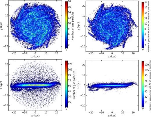
Top panels: face-on distribution of all the gas particles located within the galactic radius for the AqC5-newH galaxy simulation (left); face-on distribution of gas particles within Rgal with the AC switched off as a consequence of the implementation of our AC limiter, in the same run (right). Bottom panels: edge-on distribution of all the gas particles located within Rgal for the AqC5-newH simulation (left); edge-on distribution of gas particles within Rgal with the AC switched off because of the AC limiter (right). Plots are shown at redshift z = 0; the colour encodes the numerical density of the particles per bin.

Top four panels: projected gas (first and second panels) and star (third and fourth) density for the AqC5-newH simulation. Bottom four panels: projected gas (fifth and sixth panels) and star (bottom) density for AqC5-oldH. Left- and right-hand panels show face-on and edge-on densities, respectively. All the maps are shown at redshift z = 0. The size of the box is 55 kpc.
Particles with AC switched off mainly trace the densest and the innermost regions of the simulated disc galaxy. Thus, Figs 4 and 5 show how AC is switched off for particles that are sampling the ISM, described by sub-grid physics, whose evolution strongly affects the gas thermodynamics and dominates over the resolved hydrodynamics. In particular, both the edge-on view of the AqC5-newH galaxy (bottom-right panel of Fig. 5) and Fig. 4 (combined with information provided by Fig. 2) show how AC is instead normally acting outside the galaxy.
5.2 Effect of the new SPH scheme
In this section, we focus our attention on the results from AqC5 simulations, just stressing few differences with respect to the low-resolution case where needed. In order to investigate the significant role played by the advanced hydrodynamic scheme in the formation and evolution of a disc galaxy, we performed the comparison at both available resolutions, i.e. between runs AqC5-oldH and AqC5-newH, and AqC6-oldH and AqC6-newH (see Table 1). A more detailed study of the effect of the resolution is performed in Appendix A.
Fig. 6 introduces galaxies AqC5-newH and AqC5-oldH. The first four panels show face-on and edge-on projections of gas (top panels) and stellar (third and fourth ones) density for AqC5-newH at z = 0. The four lower panels present face-on and edge-on projections of gas (fifth and sixth panels) and stellar (bottom ones) density for AqC5-oldH, at z = 0, for comparison.
The galaxy AqC5-newH has a limited bulge and a dominant disc, with a clear spiral pattern both in the gaseous and in the stellar component. The gaseous disc is more extended than the stellar one (see also the middle-left panel of Fig. 11 and discussion below).
Fig. 7 shows the SFR as a function of the cosmic time for AqC5-newH and AqC5-oldH simulations. Here, and in the rest of this work, we only show the SFR evaluated for all stars that at z = 0 are located within Rgal. In all the figures presented and discussed in this section, results of AqC5-newH are shown in red, while those referring to AqC5-oldH are in black. The burst of SF occurring at redshift z > 3 builds up the bulge component (see M15) in the two simulated galaxies. High-redshift (z > 3) SFR is reduced when the new flavour of SPH is considered: as a consequence, the bulge component of AqC5-newH is slightly less massive (see Fig. 8, described below). Below z = 2.5, the SFR evolves differently in the two simulations. AqC5-newH has a lower SFR till z = 0.5, when the two SFRs become again comparable.

SFR as a function of cosmic time for the AqC5 simulations with the old (black) and the new (red) hydrodynamic scheme.

Stellar mass as a function of the circularity of stellar orbits at z = 0. The red curve refers to the AqC5-newH and the black curve shows the result from the AqC5-oldH simulation. The heights of the peaks located at Jz/Jcirc = 0 and at Jz/Jcirc = 1 describe the relative contributions to the total stellar mass of the galaxy from the bulge and the disc, respectively. We find B/T = 0.30 and 0.23 for AqC5-newH and AqC5-oldH, respectively.
One of the reasons of the discrepant SFR between AqC5-oldH and AqC5-newH for redshift that spans the range 2.5 > z > 0.5 lies in the presence of the time-step limiting particle wake-up scheme. This feature of the improved SPH promotes the accurate treatment of feedback (Durier & Dalla Vecchia 2012; Schaller et al. 2015; Beck et al. 2016). When the wake-up scheme is used, energy deposited by wind particles in the surrounding medium when they hydrodynamically re-couple with the ambient gas is more accurately distributed, especially to cold inflowing gas. This slows down the gas accretion on to the galaxy (or even on to the halo) and reduces the amount of fuel that is available for the disc growth (see also Fig. 9, and discussion below). We note that is an interaction of the outflow model with the wake-up feature of our new hydrodynamical scheme, and depends not only on the sub-grid model parameters but also on the details of the wake-up scheme. Here, we decided to keep the wake-up scheme and its parameter (fw, see Section 2.1) fixed. We use indeed the wake-up scheme as tested in Beck et al. (2016), where a number of hydrodynamical only tests are shown. A deeper investigation of the interaction between the wake-up and the outflows will be the subject of future studies.
Left-hand panel: MAH, i.e. the redshift evolution of the gas mass, within the virial radius. AqC5-oldH is shown in black, while the AqC5-newH simulation in red. Right-hand panel: MAH for gas within the galactic radius.
Besides the smaller amount of the accreted gas in AqC5-newH, inflowing gas is characterized by a lower (radial component of the) velocity than in AqC5-oldH (for 2.5 > z > 1): as a result, the SFR drops. Moreover, gas expelled by high-redshift outflows falls back at later times in the AqC5-newH: the SFR starts to gently rise for z < 1, and then keeps roughly constant below z < 0.5, while the SFR of AqC5-oldH is moderately declining. The final SFRs slightly overestimate that observed in typical disc galaxies (see e.g. Snaith et al. 2014, for our Galaxy). The different SF history is the result of the lower baryon conversion efficiency of AqC5-newH (see Fig. 12, right-hand panel, described below).
We then analyse the distribution of stellar circularities in order to perform a kinematic decomposition of the simulated galaxies, by separating the dispersion supported component (bulge) from the rotationally supported one (disc). Fig. 8 shows the distribution of stellar mass as a function of the circularity of star particles7 at z = 0 for the two simulations. We consider star particles within Rgal. Virial radii of the two galaxies are Rvir = 238.64 kpc (AqC5-oldH) and Rvir = 240.15 kpc (AqC5-newH). The circularity of a stellar orbit is characterized by the ratio Jz/Jcirc, i.e. the specific angular momentum in the direction perpendicular to the disc over the specific angular momentum of a reference circular orbit. This latter quantity is defined according to Scannapieco et al. (2009) as Jcirc = r × vc(r) = r(GM(<r)/r)1/2, vc(r) being the circular velocity of each star at the distance r from the galaxy centre.
The bulk of the stellar mass is rotationally supported, thus highlighting that the disc represents the dominant component. The relative contribution to the total galaxy stellar mass from the bulge and the disc components can indeed be appreciated by weighting the heights of the peaks located at Jz/Jcirc = 0 and at Jz/Jcirc = 1, respectively. The total stellar mass of AqC5-newH (4.74 × 10¹⁰ M⊙, within Rgal) is lower than that of AqC5-oldH (7.22 × 10¹⁰ M⊙); both simulated galaxies are clearly disc-dominated. Assuming that the counter-rotating stars are symmetrically distributed with zero average circularity, we estimate the bulge mass as twice the mass of counter-rotating stars. We can thus calculate the bulge over total stellar mass ratio within Rgal. We obtain B/T = 0.30 and 0.23 for AqC5-newH and AqC5-oldH, respectively. The mass of the bulge component in AqC5-newH is marginally reduced with respect to AqC5-oldH (see Fig. 7 and discussion above); the stellar mass in the disc component is decreased as well in AqC5-newH. Gas mass within Rgal for AqC5-newH is 2.91 × 10¹⁰ M⊙, the cold (T < 105 K) gas mass being 2.54 × 10¹⁰ M⊙; gas mass within Rgal for AqC5-oldH is 1.66 × 10¹⁰ M⊙, the amount of cold gas being 1.55 × 10¹⁰ M⊙.
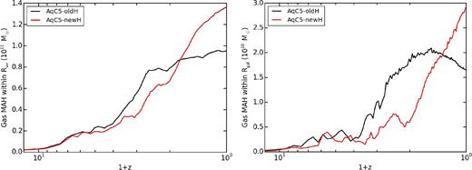
Fig. 9 describes the mass accretion history (MAH), i.e. the redshift evolution of the gas mass, within the virial radius (left-hand panel) and the galactic radius (right-hand panel). Gas accretion within Rvir is comparable in the two reference simulations up to z ≃ 4; below this redshift, the gas accretion is delayed when the new SPH implementation is adopted and then, after redshift z = 1, continues rising down to z = 0. On the other hand, the old hydrodynamic scheme reduces the gas mass accretion rate below z ≃ 2, and this is much more evident when the gas accretion within Rgal is analysed, where it is stopped below z ≃ 1. This different gas accretion pattern is one of the reasons of the differences that we found between the two AqC5 simulations. The new hydrodynamic scheme is responsible for the delay of the gas inflow, by slowing down the gas fall-back within the virial and the galactic radii. Moreover, low-redshift (z < 1) gas accretion is faster in AqC5-newH and still ongoing at z = 0: as a consequence, the stellar disc forms later and it is still growing at redshift z = 0, when fresh gas keeps accreting on the galaxy, sustaining the SF.
Fig. 10 shows the density–temperature phase diagram of all the gas particles within the virial radius for the AqC5-newH simulation (left-hand panel) and for the run AqC5-oldH (right-hand one). The mass distribution is shown at z = 0 and both single-phase and multiphase particles are taken into account. As for the temperature, it is the temperature of single-phase particles and the mass-averaged temperature for the multiphase ones. The presence of AC affects the gas particle distribution in the phase diagram: cooling properties are modified, phase-mixing is promoted. When more diffuse gas is considered, i.e. ρ < 3 × 10⁴ M⊙ kpc−3, we find that the gas is kept hotter in the AqC5-newH simulation, with a lot of gas at temperatures 3 × 10⁵ < T < 4 × 10⁶ K. At intermediate densities, i.e. 3 × 10⁴ < ρ < 4 × 10⁵ M⊙ kpc−3, and for T > 3 × 10⁵ K, we notice the presence of a large number of gas particles that have been recently heated because of stellar feedback in the AqC5-newH simulation, while in the same density and temperature regime there is a lack of these particles in the AqC5-oldH. This feature confirms the importance of the time-step limiting particle wake-up scheme in the improved SPH, as discussed above. At higher densities, above the multiphase threshold, AqC5-newH is characterized by a larger amount of multiphase and star-forming particles, as a consequence of the more active SFR at z = 0.

Phase diagrams of gas particles within the virial radius for the simulations AqC5-newH (left-hand panel) and AqC5-oldH (right-hand panel). Colour encodes the mass of gas particles per density–temperature bin. The colour scale is the same for both panels.
From these phase diagrams, we conclude that the interplay between hydrodynamical scheme and sub-resolution model plays an important role in determining the thermodynamical properties of gas particles and the resulting history of SF and feedback.
Fig. 11 shows radial profiles at z = 0 of some interesting physical properties of the two galaxies obtained with the new and the original implementation of SPH. The top-left panel describes rotation curves for AqC5-oldH (black) and AqC5-newH (red). In this panel, the solid curves describe the circular velocity due to the total mass inside a given radius, while dashed, dotted and dot–dashed curves show the different contribution of DM, stars and gas to the total curve, respectively. Both galaxies, and AqC5-newH in particular, are characterized by total rotation curves that exhibit a flat behaviour at large radii and that are not centrally peaked, thus pointing to galaxies with a limited bulge and a dominant disc component. Differences between contributions of considered components can be understood by analysing density radial profiles.
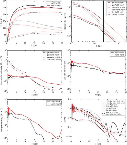
Upper panels: left: rotation curves for the AqC5 simulations with the old (black) and the new (red) hydrodynamic scheme. The solid curve describes the circular velocity due to the total mass inside a given radius. The different contribution of DM (dashed line), stars (dotted), and gas (dot–dashed) to the total curve are shown. Right: density radial profiles of gas (solid curve), stars (dotted), and DM (dashed) for the AqC5-newH and AqC5-oldH simulations. Black and red vertical solid lines mark the galactic radii of AqC5-oldH and AqC5-newH, respectively, the x-axis extending to the virial radius of the second one. Middle panels: left: surface density profiles. Solid curves describe the contribution of gas and dashed lines are the one of the stars. Right: gas temperature radial profiles. Bottom panels: left: gas pressure radial profiles. Right: radial profiles of oxygen abundance of gas (dotted curves), stars (dashed), and young stars (solid, see the text) for AqC5-newH (red) and AqC5-oldH (black). Data (grey filled circles) show the radial abundance gradient for oxygen from observations of Cepheids (Luck & Lambert 2011), according to the division in bins performed by Mott, Spitoni & Matteucci (2013). Error bars represent the standard deviation in each bin. In all the panels, results for the simulation AqC5-oldH are shown in black and for AqC5-newH in red. All the profiles are analysed at z = 0.
The top-right panel of Fig. 11 shows the density radial profiles of gas (solid), stars (dotted), and DM (dashed) in the reference simulations, out to Rvir = 240.15 kpc, the virial radius of AqC5-newH. Solid vertical red and black lines pinpoint the location of Rgal of AqC5-newH and AqC5-oldH, respectively. DM profiles only differ in the innermost regions, i.e. r < 4 kpc. Such a discrepancy is related to the different high-z (z > 3) SFR between the two simulated galaxies (see Fig. 7 ). The lower high-z SFR in AqC5-newH produces a stellar feedback associated to the SF burst that is not as strong as in AqC5-oldH: as a consequence, the DM component in AqC5-newH experiences a gentler adiabatic expansion, the feedback induced gas displacement being not as striking as in AqC5-oldH, at that epoch. This results in a higher central DM volume density in AqC5-newH. Gas and stellar density profiles have similar shapes but different normalizations. A higher gas content characterizes the AqC5-newH simulation, while the contribution of stars is more important in AqC5-oldH, as already seen in the circularity histograms (and quantified with gas and stellar masses above).
The middle-left panel of Fig. 11 shows surface density profiles. Solid and dashed curves refer to gas and to stars, respectively. The comparison between the gas contribution in the two simulations further shows that AqC5-newH has a higher gas content. Moreover, the size of the gas disc is more extended and the gas mass surface density is larger in the innermost regions. The higher gas content in AqC5-newH at z = 0 is due to the fact that we have a larger amount of gas that is infalling towards the galaxy at z < 1 with the new hydrodynamic implementation (see Fig. 9), thus being consistent with the increasing low-z SFR shown in Fig. 7. Stellar surface density profile is higher for AqC5-oldH, and this is in agreement with the fact that high-redshift expelled gas fell back on this galaxy at earlier times and produced more stars, while this process is still ongoing in AqC5-newH.
The middle-right and bottom-left panels of Fig. 11 show the radial profiles of gas temperature and pressure, respectively. Discs obtained with the improved SPH formalism are hotter and more pressurized in the innermost regions. The higher pressure in AqC5-newH with respect to AqC5-oldH is a direct consequence of the higher gas surface density in the galaxy simulated with the new hydrodynamic scheme (see discussion above). Temperature and pressure profiles can be further illustrated by considering the phase diagrams of gas particles shown in Fig. 10 and discussed above: we indeed see that in AqC5-newH there is a larger number of particles having a higher temperature, when both the low- (ρ ≲ 5 × 10⁵ M⊙ kpc−3) and the high-density (ρ ≳ 5 × 10⁵ M⊙ kpc−3) regimes are considered. This holds in particular for multiphase particles, thus probing the higher temperature and pressure in the innermost regions of AqC5-newH.
The last panel of Fig. 11 describes metallicity radial profiles of the two simulations. We compare our simulated metallicity profiles with high-quality data measured for stars in our Galaxy. We note that the current simulations are not aimed at modelling the MW; the goal of the comparison is to understand if simulated results are in broad agreement with observations of a typical disc galaxy like our MW. We consider radial profiles of oxygen abundance (that is an accurate and reliable tracer of the total metallicity) in gas and stars for AqC5-newH (red) and AqC5-oldH (black). Data (grey filled circles) show the radial abundance gradient for oxygen from observations of Cepheids (Luck & Lambert 2011), according to the division in bins as a function of the Galactocentric distance performed by Mott et al. (2013). Error bars represent the standard deviation computed in each bin, whose width is 1 kpc. Dotted and dashed curves depict the oxygen abundance radial profile from all the gas and star particles within Rgal at z = 0, respectively. We also consider oxygen abundance radial profiles (solid curves) by limiting the considered stars to those that have been formed after z ≲ 0.007, i.e. less than ∼100 Myr ago. Cepheids are indeed young stars (estimated age of ≲ 100 Myr, Bono et al. 2005): solid curves allow a fair comparison with observations (we will therefore focus on them in the following analysis). We find a good agreement with observations: the slope of the radial profile predicted by considering only young stars in AqC5-newH, for distances from the galaxy centre spanning the range 5 ≲ r ≲ 15 kpc, well conforms to the trend suggested by observations. The ability to recover well the slope predicted by observations highlights the effectiveness of our sub-resolution model to properly describe processes that affect the spread and the recycling of metals. We also note that there is a flattening of profiles in simulations for distances r ≲ 5 kpc from the galaxy centre. The normalization of the oxygen abundance profile of young stars in AqC5-newH is consistent with observations within the error bars (despite a slight overestimate by ∼0.05 dex, while the overestimate is about ∼0.1 dex when AqC5-oldH is considered). However, a different normalization of the abundance profiles in simulations with respect to the observed ones is expected, as the normalization of the profiles in simulations is affected by many aspects (e.g. uncertainties related to the yields and IMF). On the other hand, their slope can be directly compared to that of the observed abundance gradients.
The left-hand panel of Fig. 12 displays the stellar Tully–Fisher relation for the AqC5-newH (red) and AqC5-oldH (black) simulations. We measure the circular velocity at a distance of 8 kpc from the galaxy centre and consider the galaxy stellar mass within the galactic radius. We also plot observational data (Courteau et al. 2007; Verheijen 2001; Pizagno et al. 2007), the best fit to them (Dutton et al. 2011) and results from the following simulations of late-type galaxies: the purple triangle is the AqC5 from Marinacci et al. (2014), the blue triangle is the AqC5 from Aumer et al. (2013), and the orange filled square shows Eris simulation from Guedes et al. (2011). Green triangles are AqC5 galaxies from the Aquila comparison project (Scannapieco et al. 2012, simulations G3-TO (light green), G3-CS (medium green), and R-AGN (dark green)). The brown diamond shows where the MW is placed in the Tully–Fisher relation diagram. We do not intend to claim that AqC is a model of the MW, our Galaxy being included only for completeness. As for the properties of the MW, we adopted the following values: 6.43 × 10¹⁰ M⊙ is the total stellar mass, 250 km s−1 is the circular velocity (evaluated at 8 kpc, to be consistent with our analysis), and 1.85 × 10¹² M⊙ is the halo mass (McMillan 2011; Bhattacharjee et al. 2014; Zaritsky & Courtois 2017). We note that our galaxies are located in the upper edge of the region traced by observational results, thus highlighting a predicted circular velocity slightly higher than the one expected from observations at the considered stellar mass. As discussed in M15, this appears to be a feature shared among several similar simulations of late-type galaxies. ICs likely play a role in the aforementioned shift, rather than resolution.

Left-hand panel: Tully–Fisher relation for the AqC5-newH (red) and AqC5-oldH (black) simulations. We use the circular velocity at a distance of 8 kpc from the galaxy centre as a function of the galaxy stellar mass within the galactic radius. Grey crosses, diamonds, and plus symbols are observations from Courteau et al. (2007), Verheijen (2001), and Pizagno et al. (2007), respectively, the solid line providing the best fit (Dutton et al. 2011). Other coloured symbols refer to the following simulations of late-type galaxies: the purple triangle is the AqC5 from Marinacci et al. (2014), the blue triangle is the AqC5 from Aumer et al. (2013), the orange filled square shows Eris simulation from Guedes et al. (2011), and green triangles are AqC5 galaxies from the Aquila comparison project (Scannapieco et al. 2012, simulations G3-TO (light green), G3-CS (medium green), and R-AGN (dark green)). Right-hand panel: Baryon conversion efficiency of the two disc galaxies at z = 0. Blue solid line shows the stellar-to-halo mass relation derived by Guo et al. (2010), with the shaded blue region representing an envelope of 0.2 dex around it. Purple solid curve describes the fit proposed by Moster et al. (2010), with 1σ uncertainty (shaded envelope) on the normalization. Brown diamonds show where the MW is located in the Tully–Fisher relation and in the stellar-to-halo mass relation plots. We include our Galaxy for completeness. Properties of MW according to McMillan (2011), Bhattacharjee, Chaudhury & Kundu (2014), and Zaritsky & Courtois (2017).
The right-hand panel of Fig. 12 shows the baryon conversion efficiency of the two disc galaxies at z = 0. Blue solid line shows the stellar-to-halo mass relation derived by Guo et al. (2010), with the shaded blue region representing an interval of 0.2 dex around it (as done in Marinacci et al. 2014, and in M15). Purple curve describes the fit (solid line) proposed by Moster et al. (2010), with 1σ uncertainty (shaded envelope) on the normalization. The simulation performed with the new SPH implementation is characterized by a lower baryon conversion efficiency, that is in good agreement with both the predictions by Moster et al. (2010) and Guo et al. (2010). As discussed above, this reflects on the lower stellar mass of the new galaxy.
As for the comparison between AqC5-oldH and AqC5-newH simulations, the key differences can be interpreted as an effect of the different MAH: gas accretion within the virial and galactic radii is delayed in AqC5-newH. In this simulation, we still have fresh gas that is infalling towards the galaxy centre at z < 1. In general, we are able to obtain a disc-dominated galaxy with both the old and the new hydrodynamic schemes. The free parameters of our sub-grid model had to be re-tuned when the improved SPH implementation has been adopted.
5.3 Changing the galactic outflow model
5.3.1 Tuning the models
In this section, we compare the results obtained from the three implementations of galactic outflows described in Section 3, and compare them to the original one presented by M15. We remind that all the differences we present in this section are only due to the change in the outflow model, being the ICs, the code, the SPH implementation and the MUPPI SF model exactly the same in all cases. Note that we kept fixed the scheme for the thermal energy release of MUPPI. All the changes only concern the distribution of the fraction of SN energy that is provided in kinetic form in the original model.
For each of the three outflow models, we carried out a detailed exploration of the corresponding parameter space. To select our preferred set of parameters, we mainly focused on those simulations that produce the most prominent stellar disc component, as evaluated by visual inspection and by comparing the circularity histograms, as those shown in Fig. 13. We also analysed the galactic SFRs, as those shown in Fig. 14, trying to minimize the high-redshift SF burst, in order to prevent a too large amount of late gas infall and, consequently, a too high low-redshift SFR. We did not succeed in simultaneously calibrating other properties of our simulated galaxies, such as the B/T ratio or the total stellar mass (or one between the disc or the bulge stellar mass). However, as we will show below, our main point is that galaxy properties are deeply linked to the selected outflow model: it is very difficult to obtain the same set of properties by simply tuning the model parameters.

Stellar mass as a function of the circularity of stellar orbits at z = 0. The red curve refers to the AqC5-newH run, the green one to AqC5-FB1, the blue curve identifies AqC5-FB2, and the purple one AqC5-FB3. The values of the B/T ratios are: 0.30, 0.19, 0.35, and 0.54, respectively.

SFRs for the AqC5-FB1, AqC5-FB2, and AqC5-FB3 simulations, compared with that of AqC5-newH. Colours are as in Fig. 13. Results refer to z = 0.
We performed an accurate exploration of the models’ parameter space mainly using the low-resolution AqC6 ICs. When needed, we slightly re-tuned some of the parameters at the higher resolution of the AqC5 ICs. In this section, we only show results for our AqC5 best cases. The procedure for parameter tuning is described in Appendix B.
Our FB1 model is an implementation of the model originally introduced by Dalla Vecchia & Schaye (2012), in the context of our MUPPI SF and ISM model. Here, the relevant parameters are the temperature jump ΔT, and the fraction of SNII energy available to power the outflows, ffb, kin, i.e. the feedback efficiency. We adopt a temperature jump that depends on the density of gas particles that are eligible to produce feedback, as detailed in Section 3.1 (see also Appendix B for results of a simulation where we fix the temperature jump to the value of T = 107.5 K). As far as the feedback efficiency is concerned, we adopted the density- and metallicity-dependent feedback efficiency used in the reference Eagle simulation (Schaye et al. 2015), as discussed in Section 3.1. Such a choice successfully produces a disc-dominated galaxy at redshift z = 0, even if this galaxy is characterized by high low-redshift gas MAH and resulting SFR (see Figs 15, 14, and discussion in Section 5.3.2). None the less, we prefer to consider the model adopting this feedback efficiency (equation 11) as reference FB1 simulation: we then discuss in Appendix B how different choices for ffb, kin can reduce the amount of gas available for the low-z phase of disc formation, thus regulating the SFR at z = 0.

Gas MAH for AqC5-FB1, AqC5-FB2, and AqC5-FB3, compared with the result of AqC5-newH. Colours are as in Fig. 13. Left-hand panel shows the gas MAH within the virial radius, and right-hand panel within the galactic radius.
Energy provided by SF is distributed according to Dalla Vecchia & Schaye (2012): first, we calculate the SNII energy release of the whole stellar population. Then, when a star is spawned, we use it to heat the surrounding gas. In principle, such mechanism of delivering energy contrasts with the continuous SFR of MUPPI model. In our sub-grid model, energy provided by SNe is indeed computed by using the energy contributed by the virtual stellar component in multiphase gas particles in each time-step, regardless of the moment in which the spawning of a star particle occurs. This results in a gradual way of distributing and releasing energy. On the other hand, if the whole amount of energy is released impulsively when a star is really spawned, the feedback turns out to be more effective. The gradual way of distributing energy does not allow us to produce disc-dominated galaxies when the FB1 galactic outflow model is adopted, since the stellar feedback is not effective enough to prevent an excessive high-redshift SF burst. This set of choices allows us to produce an AqC5-FB1 galaxy with a dominant disc component.
The FB2 scheme is a modification of the original MUPPI outflow model. In the process of tuning this model's parameters, we had to reduce the value of the SNII energy faction down to ffb, kin = 0.12 and the probability of a gas particle to become a wind one to P = 0.03, in order to account for the fact that this scheme does not limit the search of available wind particles to a cone but uses the whole smoothing sphere.
Finally, results for our FB3 scheme are shown with parameters η = 3.0 and ffb, kin = 2.0. In Appendix B, we discuss our choice of the parameter ffb, kin, that is the parameter to which our model is most sensitive. There, we also refer to Springel & Hernquist (2003), whose model this galactic outflow scheme is inspired. Here, we note that the higher is the value of the mass loading factor (values of η ranging between 0.5 and 8), the narrower and more reduced is the high-redshift SF burst, thus shortening the phase of bulge formation and limiting bulge size accordingly. Observations of low-redshift kpc-scale neutral gas outflows suggest a value for the mass loading factor that slightly exceeds unity (Cazzoli et al. 2014).
5.3.2 Comparing results
In this section, we discuss results obtained using our four galactic outflow models, the original one and those described in Section 3. We focus on the following properties of the simulated galaxies: circularity of stellar orbits, SFRs, gas MAHs, rotation curves, Tully–Fisher relation and baryon conversion efficiencies, metallicity, and surface density profiles.
In Fig. 13, we show the circularities for all of our models, at redshift z = 0. In all cases, we obtain rotationally supported galaxies. However, the bulge over total mass ratio changes significantly with the outflow model, with B/T = 0.30, 0.19, 0.35, and 0.54 for the original model, FB1, FB2, and FB3, respectively.8 The total stellar mass of the galaxy (the integral of the circularity histogram) does change, too. Total stellar masses within Rgal for AqC5-newH, AqC5-FB1, AqC5-FB2, and AqC5-FB3 are 4.74 × 10¹⁰ M⊙, 9.34 × 10¹⁰ M⊙, 3.29 × 10¹⁰ M⊙, and 2.94 × 10¹⁰ M⊙, respectively. Galactic radii are 24.01 kpc for AqC5-newH, 24.76 kpc for AqC5-FB1, 23.90 kpc for AqC5-FB2, and 23.58 kpc for AqC5-FB3.
Fig. 14 shows the SFRs obtained for our four implementations of the outflow model, as a function of the cosmic time. SFRs are computed by considering all stars within Rgal at z = 0. The SFR of all models is comparable at high (z > 3) redshifts. Bulges of simulated galaxies form at these epochs. At later times, during the disc formation phase, the behaviour of our outflow models differs. FB1 scheme has an SFR that is slightly higher than the other models between 3 > z > 2, thus producing a further growth of the bulge, that is the most massive one. The SFR of this model has then a drop; at z ≃ 0.7 it starts to rapidly increase again, and it reaches the roughly constant value of ≃ 20 M⊙ yr−1 from z ≃ 0.35 on, i.e. over the last ∼4 Gyr. Schaye et al. (2015) predict the SFR to be at most ≃8 M⊙ yr−1 for a galaxy with a stellar mass slightly lower than 8 × 10¹⁰ M⊙ at z = 0.1 (this value corresponds to the upper edge of the 1σ uncertainty of their fig. 11). Our Galaxy (whose stellar mass is 7.39 × 10¹⁰ M⊙ at z = 0.1) has therefore an SFR in excess of that predicted by Schaye et al. (2015) by a factor of 2.5. However, unlike in Schaye et al. (2015), our simulations do not include SMBHs (supermassive black holes) and the ensuing AGN (active galactic nucleus) feedback: AGN feedback is indeed expected to play a role in reducing low-redshift SFR (in Appendix B, we show how we regulated the low-z SFR with a different choice of ffb, kin). Fig. 14 highlights how different prescriptions for the SF impact on final results, even when the same galactic outflow model is adopted. Both FB2 and FB3 schemes do show a drop in the SFR below z = 2 with respect to AqC5-newH. In the FB2 case, SFR rises again after z ≃ 0.5, while it remains below ∼2 M⊙ yr−1 for FB3. This is clearly at the origin of the higher B/T ratios produced by these two schemes: the early-forming bulge component is similar to that of AqC5-newH, but the disc formation phase is delayed or suppressed.
The reason for the different behaviour of the SFR among models is further illustrated by Fig. 15. Here, we show the gas MAH on to the main progenitor of the galaxy as a function of the redshift. We have already shown in Fig. 9 a comparison of the gas MAH using the old and the new SPH implementation, and found a delay in the gas fall-back when we use the new scheme with respect to the old one. Here, the qualitative behaviour of the MAH is similar for all of our four galactic outflow models for z ≳ 2, both within the virial (left-hand panel) and the galactic (right-hand panel) radii. FB1 has the highest gas accretion rate from z ≃ 1.5 on. This feature highlights that this galactic outflow model is not as effective as the others in preventing gas accretion and explains the highest low-redshift SFR and final stellar mass of the galaxy simulated with this scheme. FB2 gas MAH closely follows that of our original scheme at the virial radius, but the gas accretion rate within Rgal at low redshift (below z ∼ 2) is significantly lower. We interpret this as the evidence that this kind of feedback is more effective at low redshift, generating strong outflows that stop gas from fuelling the disc growth. FB3 is even more effective in expelling gas from the galaxy, and at z ≲ 1 also from the halo. In fact, it has the lowest SFR, the smallest disc component and, as a consequence, the highest value of the B/T ratio.9
In Fig. 16, we show the circular velocity profiles for all the schemes. AqC5-newH, FB2, and FB3 models have profiles that are flat at large radii, thus confirming their ability to prevent the formation of a strong baryonic concentration at the centre. FB1 scheme produces a galaxy whose stellar component of the rotation curve has the most pronounced peak at small radii (r ≲ 5 kpc): this is related to the larger mass of the bulge that is produced in this case. The morphology of this galaxy, with prominent stellar spiral arms, originates the peak of the velocity profile of the FB1 model, at r ≃ 8 kpc (see the stellar density profile in Fig. 17, too). The normalization of the circular velocity profiles straightforwardly follows the different stellar (see above) and gas (see below) masses of the four simulations.

Rotation curves at z = 0 for AqC5-FB1, AqC5-FB2, and AqC5-FB3, compared with that of AqC5-newH. Colours as in Fig. 13. The solid curves describe the circular velocity due to the total mass inside a given radius. The different contribution of DM (dashed line), stars (dotted), and gas (dot–dashed) to the total curve are shown.

Left-hand panel: surface density profiles for simulations AqC5-newH (red), AqC5-FB1 (green), AqC5-FB2 (blue), and AqC5-FB3 (purple). Solid curves describe the contribution of gas and dashed lines the one of the stars. Right-hand panel: radial profiles of oxygen abundance in young stars (see the text) for the four simulations. Data (grey filled circles) show the radial abundance gradient for oxygen from observations of Cepheids (Luck & Lambert 2011), according to the division in bins as a function of the Galactocentric distance performed by Mott et al. (2013). Error bars represent the standard deviation computed in each bin. All the profiles are analysed at z = 0.
The left-hand panel of Fig. 17 shows surface density profiles of the four simulated galaxies. Dashed and solid curves refer to stars and to gas, respectively. Total gas masses within Rgal for AqC5-newH, AqC5-FB1, AqC5-FB2, and AqC5-FB3 are 2.91 × 10¹⁰ M⊙, 3.33 × 10¹⁰ M⊙, 2.07 × 10¹⁰ M⊙, and 8.82 × 10⁹ M⊙, respectively. Total gas masses within Rvir for AqC5-newH, AqC5-FB1, AqC5-FB2, and AqC5-FB3 are 1.36 × 10¹¹ M⊙, 1.48 × 10¹¹ M⊙, 1.36 × 10¹¹ M⊙, and 9.75 × 10¹⁰ M⊙, respectively. Gas masses directly come from the different gas MAHs within Rvir and Rgal (see Fig. 15). AqC5-newH has both the most extended gas disc and the stellar component that extends farthest from the galaxy centre. AqC5-FB1 has the largest gas mass surface density in the innermost regions. Gas surface density profiles of AqC5-FB1, AqC5-FB2, and AqC5-FB3 exhibit a bump at the edge of the gas disc (at distances of 7, 10, and 6 kpc, respectively). In particular for AqC5-FB1 and AqC5-FB2, it is possible to note a corresponding excess in the stellar surface density. This is the effect of high angular momentum gas infalling within Rgal at low redshift. The shallower decrease in the stellar surface density profiles is a consequence of the enhancement of the SF due to the recently accreted gas. The infalling gas is material ejected from the forming halo – due to the high-redshift (z ≳ 3) SF burst that formed the bulge – with a low angular momentum. After acquiring angular momentum from halo gas (Brook et al. 2012; Übler et al. 2014; Teklu et al. 2015; Genel et al. 2015), the expelled material fell back, in a way regulated by the stellar feedback. As for AqC5-FB3, the gas fall-back occurred at earlier times than in AqC5-FB1 and AqC5-FB2 (see Fig. 15 and discussion above), where instead the process is still ongoing.
The right-hand panel of Fig. 17 shows the metallicity radial profiles of the four simulations, where we consider radial profiles of oxygen abundance in stars (within Rgal) that are younger than ∼100 Myr, in order to make a fair comparison with observations (as discussed in Section 5.2). Data (grey filled circles) are the same as in the last panel of Fig. 11. Negative radial abundance gradients are recovered for all the models, in line with observational results. The agreement between oxygen abundance radial profiles predicted by different simulations and observations demonstrates the effectiveness of a sub-resolution model (and in particular of a galactic outflow model) to properly describe the chemical enrichment of the galaxy at different positions. We see that the galactic outflow model of AqC5-newH and FB2 well reproduce the slope of observed radial abundance profiles. The slope of the profile in AqC5-FB1 is slightly flatter than in observations. We note that the normalization of radial abundance profiles in simulations is a delicate aspect (as discussed in Section 5.2); none the less, the normalization of the oxygen abundance profile in both the AqC5-newH and AqC5-FB2 simulations is consistent with the observed abundance gradient within the error bars. The metallicity radial profile predicted by the AqC5-FB1 simulation shows an oxygen abundance lower than observations in the inner regions (r ≲ 10 kpc). The metal content of young stars throughout the galaxy is more homogeneous: this galactic outflow model is able to promote a more efficient spread of metals from stars to the surrounding gas. As for the FB3 model, it does not succeed in reproducing observations. The AqC5-FB3 galaxy has a limited stellar disc (see Fig. 17, left-hand panel), it is characterized by a low SFR (Fig. 14) and a reduced gas MAH (Fig. 15) below z ∼ 1: as a consequence, a lower amount of metals has been produced in a confined region (subsequently generated stars being richer in heavy metals than previous ones). As for the relative difference between slopes and normalizations of profiles in simulations AqC5-newH and AqC5-FB2, metals are less locked into stars in AqC5-newH with respect to AqC5-FB2.
Fig. 18 shows the position of the four simulated galaxies in the Tully–Fisher diagram. Also in this case, as already discussed in Section 5.2, all the simulated galaxies lie close to the upper limit of the region allowed by observations. AqC5-FB1 galaxy lies just outside the region identified by the scatter of the observed data: this is a consequence of its peaked rotation curve (Fig. 16). Rotation velocity scales with the stellar mass of the simulated galaxies, thus the position in the diagram of our four galaxies just relates with their stellar mass.

Tully–Fisher relation at z = 0 for AqC5-FB1, AqC5-FB2, and AqC5-FB3, compared with that of AqC5-newH. Colours are the same used in Fig. 13. We use the circular velocity at a distance of 8 kpc from the galaxy centre as a function of the galaxy stellar mass within the galactic radius. Grey symbols are as in Fig. 12.
Finally, in Fig. 19, we show the position of our simulations in the baryon conversion efficiency plot. FB1 is characterized by a baryon conversion efficiency that slightly exceeds the uncertainty contour of the prediction by Guo et al. (2010) and that overestimates the one by Moster et al. (2010). FB2 shows a baryon conversion efficiency lower than the expectations from Guo et al. (2010) and Moster et al. (2010), and also FB3 underproduces stars. We note that the lower the baryon conversion efficiency of simulated galaxies is, the larger their B/T (see Fig. 13).
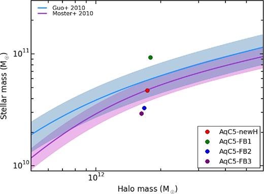
Baryon conversion efficiencies at z = 0 for AqC5-FB1, AqC5-FB2, and AqC5-FB3, compared with that of AqC5-newH. Colours are as in Fig. 13. Blue solid line shows the stellar-to-halo mass relation derived by Guo et al. (2010), with the shaded blue region representing an envelope of 0.2 dex around it. Purple solid curve describes the fit proposed by Moster et al. (2010), with 1σ uncertainty (shaded envelope) on the normalization.
A general result of this section is that the observational properties of the simulated galaxies are sensitive to the details of the different outflow models, even when they are implemented within the same SF scheme. Some of these properties, for instance the bulge mass and (to a lower extent) the radial dependence of the rotation velocity (at large radii) are relatively stable against the considered implementations of galactic outflow model. On the other hand, the prominence of the disc component is highly sensitive to the implemented model and, more specifically, to the timing of the gas fall-back and the mass of the gas involved. In fact, a feedback model that is successful in producing a disc-dominated galaxy should be able to regulate the pristine SF, which is responsible for the creation of the bulge component, and, at the same time, not to allow a too late gas fall-back, that would turn into a too high SFR at z = 0. The results of our simulations confirm that this represents a non-trivial requirement on galactic outflow models to be implemented in cosmological simulations of galaxy formation.
6 SUMMARY AND CONCLUSIONS
In this paper, we presented a suite of cosmological simulations of a MW-sized halo (Mhalo, DM ≃ 2 × 10¹² M⊙), namely Aquila C5 (Springel et al. 2008), using the TreePM+SPH gadget3 code. As a first aim of our analysis, we coupled a sub-resolution SF and stellar feedback model, called MUPPI (Murante et al. 2015, M15), with an improved implementation of SPH that includes a high-order interpolating kernel, an improved treatment of AV and an AC term that promotes mixing at gas interfaces (Beck et al. 2016). As a second goal, we implemented three different models for galactic outflows, besides the original model presented by M15, and used them to re-simulate the same ICs with the same SF prescription. For each scheme, we tuned the relevant model parameters by carrying out an exploration of their respective parameter space (see Appendix B). To choose the reference values of the parameters, we used the criterion based on maximizing the stellar disc component, both by visual inspection and by plotting the circularity histograms. Our simulations do not include AGN feedback.
The key features of our galactic outflow models are the following:
In our original scheme, each particle ending its multiphase stage has a probability of receiving kinetic energy from neighbour star-forming particles, providing that it is inside a cone centred on the star-forming particles and directed towards the least-resistance direction.
FB1 is a stochastic thermal feedback model based on Dalla Vecchia & Schaye (2012). It is here implemented within our sub-resolution model for the ISM and SF, different from the original one by Dalla Vecchia & Schaye (2012).
FB2 is a kinetic stellar feedback scheme, where the ISM is isotropically provided with energy that triggers galactic outflows.
FB3 is a feedback model where we directly impose the mass loading factor and stochastically sample the outflowing mass. SN energy and SFRs are collected during the multiphase stage of gas particles, thus accounting for the evolution of the ISM. This scheme is inspired by Springel & Hernquist (2003).
In order to successfully introduce the improved SPH implementation in cosmological simulations adopting the sub-resolution model MUPPI, we switched off AC for both multiphase and wind particles, and implemented a switch that allows former multiphase particles to artificially conduct whenever some conditions on their temperature are met. In fact, the physical state of the ISM is determined by continuous energy injections due to the sub-grid model. This results in a particle-by-particle difference in temperature and density. AC acts in mixing internal energy, contrasting the effect of the sub-grid model. The new switch suppresses AC for those particles that are sampling the non-uniform thermal structure of the galaxy, where the sub-resolution physics accounts for the evolution of the ISM.
Our main results can be summarized as follows.
MUPPI is able to produce a disc galaxy using the AqC5 ICs, also when coupled with the improved SPH scheme. The simulated galaxy has a flat rotation velocity profile (flatter than the one of the galaxy simulated with the previous SPH implementation), a low value of the B/T ratio, extended gaseous and stellar discs, baryon conversion efficiency, and position on the Tully–Fisher plot in broad agreement with expectations. However, we note that significant differences arise with respect to the results obtained by adopting the standard SPH scheme. Using our new SPH solver introduces a delay in the gas fall-back that causes the stellar disc to form later, and the simulated galaxy to have a relatively higher low-redshift SFR.
Changing the outflow model does affect the properties of the simulated galaxies at redshift z = 0. Some of them are relatively stable, e.g. the high-redshift (z ≳ 3) SFR which determines the present-day stellar mass of the bulge. However, the majority of the properties, in particular the prominence of the disc component, shows a sensitive dependence on the employed outflow model.
FB1 model generates the galaxy with the largest stellar mass, a strong disc component, high SFR at redshift below z ≃ 0.7. FB2 model has a smaller stellar mass at z = 0 with respect to our reference outflow scheme, and shows a drop in SFR between z = 2 and 0.3. FB3 model strongly suppresses SF after z = 2, producing in turn the lowest value of the B/T ratio.
The different behaviour of our outflow models can be understood in terms of gas MAH. FB1 almost always has the highest gas MAH; FB2 shows an MAH similar to that of our reference model within the virial radius, but lower within the galactic radius; on the other hand, FB3 is too effective in quenching the gas fuelling of the disc. In this latter outflow model, the outflowing gas is kept inside the halo, but away from the galactic radius.
Our analysis demonstrates and quantifies the strong interplay between details of the hydrodynamic scheme and the sub-resolution model describing SF and feedback. The sub-resolution model plays a fundamental role in determining the properties of simulated galaxies and the exact values of free parameters entering into this model can significantly change with the hydrodynamic solver. The hydrodynamic scheme remarkably affects properties of simulated galaxies (stellar mass is the quantity that is affected the most) and highly regulates gas inflow and outflow across cosmic time. Moreover, the higher the resolution is, the more sensitive to the accuracy of the hydrodynamic solver properties of simulated galaxies are (see Appendix A).
Our results further show that the sub-resolution prescriptions adopted to generate galactic outflows are the main shaping factor of the stellar disc component at low redshift (when the hydrodynamic scheme is held fixed). In particular, the timing of the gas fall-back after its expulsion from the forming halo at high redshift is of paramount importance, together with the ability of a given model to tune or even quench the cosmological infall of gas from the large-scale environment. For this reason, a detailed comparison between simulation results and observations of the properties of the circumgalactic medium at different redshifts should provide invaluable information on the outflow/inflow gas properties and, therefore, on the history of feedback. Another interesting direction of investigation will be to compare the properties of simulated galaxy populations (instead of those of a single galaxy), obtained by adopting one or more of our outflow models, with observations.
Acknowledgements
We thank the anonymous referee for a prompt, careful, and constructive report. We are greatly indebted to Volker Springel for giving us access to the developer version of the gadget3 code. We acknowledge Francesca Matteucci and Emanuele Spitoni for useful discussions and for providing observational data of radial abundance gradient for oxygen. This work received financial support from the PRIN-MIUR 201278X4FL Grant, the PRIN-INAF 2012 ‘The Universe in a Box: Multi-scale Simulations of Cosmic Structures’ Grant, the INFN INDARK Grant, and ‘Consorzio per la Fisica’ of Trieste. AMB acknowledges support by the DFG cluster of excellence ‘Universe’, the DFG research unit 1254 and the Leibniz–Rechenzentrum with computing time assigned to the project ‘pr92ju’. Simulations were carried out using Galileo at CINECA (Italy), with CPU time assigned through Italian SuperComputing Resource Allocation (ISCRA) proposals and an agreement with the University of Trieste, PICO at CINECA through our expression of interest, and ULISSE at SISSA.
The local signal velocity |$v^{\rm sign}_{\rm i}$| is the maximum value that the pairwise signal velocity |$v^{\rm sign}_{\rm ij}$| assumes within the smoothing length hi among different particle pairs. The pairwise signal velocity reads: |$\, v^{\rm sign}_{\rm ij} =\: c_{\rm i}^{\rm s} + c_{\rm j}^{\rm s} + \beta \mu _{\rm ij}\,$|, where cs is the sound speed of each particle, μij = vij · xij/xij, vij being the difference of velocity between particles i and j, and β = 3 has been chosen.
Multiphase particles are also eligible particles. Thermal energy is deposited in each particle over all the gas mass, i.e. not only in the hot phase. Moreover, if a gas particle that has been selected to receive energy was in a multiphase stage, then it is forced to exit it.
We show and discuss results of a simulation where we fix the temperature jump to the reference value of T = 107.5 K in Appendix B.
The index k labels gas particles within the smoothing length of each star-forming particle i; note that each energy-receiving gas particle j can have many star-forming particles inside its smoothing length.
We consider virial quantities as those calculated in a sphere that is centred on the minimum of the gravitational potential of the halo and that encloses an overdensity of 200 times the critical density at present time.
We define here the galactic radius as one-tenth of the virial radius, i.e. Rgal = 0.1Rvir. We choose this radius Rgal in order to identify and select the region of the computational domain that is dominated by the central galaxy.
Numbers of DM, gas, and star particles within Rvir at z = 0 are 710150, 362648, and 692125 for AqC5-newH, respectively, and 691717, 252660, and 895657 for AqC5-oldH.
We remind that our estimate for B/T ratio could also include satellites, stellar streams, contribution from bars, etc., within Rgal. Therefore, our B/T values should not be directly compared with observational photometric estimates.
We show, for each galactic outflow model, the simulation that produces the best results in terms of circularity histogram and SFR. Any shortfalls of each model is therefore a direct result of how the outflow is described and cannot be ascribed to an unreliable tuning of the parameters.
We also investigated the effect of a smoother transition for the redshift evolution of the feedback efficiency. We verified that, by adopting the following analytical expression:
REFERENCES
APPENDIX A: EFFECT OF THE RESOLUTION
In this appendix, we discuss how our main results change when we decrease the mass resolution by a factor of ∼10 (see Table 1).
Table A1 lists the set of simulations that we analyse in Appendices A and B. We do not report again here simulations already introduced in Tables 1 and 3. The simulation AqC6-newH that has been introduced in Tables 1 and 2 is now labelled as AqC6-newH_p003. The simulation AqC5-FB3 that had been introduced in Table 3 is now labelled as AqC5-FB3_fk2.0.
| Simulation | Parameter ffb,kin or Pkin | Outflow model | Hydro scheme |
|---|---|---|---|
| AqC6-newH_p003 | Pkin = 0.03 | M15a | New |
| AqC6-newH_p005 | Pkin = 0.05 | M15 | New |
| AqC5-FB1f 2.0-1.0 | Equation (B1) with | FB1 | New |
| |${f_{\rm fb, kin}}^{\rm max}_{\rm min}={}^{2.0}_{1.0}$| | |||
| AqC6-FB1f Eagle | Equation (7) of | FB1 | New |
| Schaye et al. (2015) | |||
| for ffb,kin (see the text) | |||
| AqC6-FB1- ΔTfix | ffb,kin: equation (7) of | FB1 | New |
| Schaye et al. (2015); | |||
| ΔTfix = 107.5 K | |||
| AqC6-FB1f 1.0 | ffb,kin = 1.0 | FB1 | New |
| AqC5-FB3_fk2.0 | ffb,kin = 2.0 | FB3 | New |
| AqC5-FB3_fk0.5 | ffb,kin = 0.5 | FB3 | New |
| AqC5-FB3_fk0.25 | ffb,kin = 0.25 | FB3 | New |
Note.aMurante et al. (2015).
| Simulation | Parameter ffb,kin or Pkin | Outflow model | Hydro scheme |
|---|---|---|---|
| AqC6-newH_p003 | Pkin = 0.03 | M15a | New |
| AqC6-newH_p005 | Pkin = 0.05 | M15 | New |
| AqC5-FB1f 2.0-1.0 | Equation (B1) with | FB1 | New |
| |${f_{\rm fb, kin}}^{\rm max}_{\rm min}={}^{2.0}_{1.0}$| | |||
| AqC6-FB1f Eagle | Equation (7) of | FB1 | New |
| Schaye et al. (2015) | |||
| for ffb,kin (see the text) | |||
| AqC6-FB1- ΔTfix | ffb,kin: equation (7) of | FB1 | New |
| Schaye et al. (2015); | |||
| ΔTfix = 107.5 K | |||
| AqC6-FB1f 1.0 | ffb,kin = 1.0 | FB1 | New |
| AqC5-FB3_fk2.0 | ffb,kin = 2.0 | FB3 | New |
| AqC5-FB3_fk0.5 | ffb,kin = 0.5 | FB3 | New |
| AqC5-FB3_fk0.25 | ffb,kin = 0.25 | FB3 | New |
Note.aMurante et al. (2015).
We now focus on simulations AqC6-oldH, AqC6-newH_p003, AqC6-newH_p005, and we contrast their results with those of AqC5-oldH and AqC5-newH that we have analysed in Section 5.2.
The four upper panels of Fig. A1 show face-on and edge-on projections of gas (top panels) and stellar (third and fourth ones) density for the AqC6-newH_p003 galaxy simulation, at z = 0. The four lower panels depict face-on and edge-on projections of gas (fifth and sixth panels) and stellar (bottom ones) density for AqC6-oldH, at z = 0. The reference system has been rotated as described for Fig. 5. AqC6-newH_p003 is a clearly disc-dominated galaxy, and a spiral pattern is evident, especially in the gas component. The gaseous disc of the galaxy produced by adopting the improved hydrodynamic scheme is more extended than the stellar one at this resolution, too. Continuing to focus on the galaxy simulated with the new SPH, it is possible to notice how the density in the outer part of the gaseous halo is no longer resolved above a given height on the disc plane (see top-right panel) at this resolution, with respect to Fig. 6. Moreover, both the gaseous and the stellar disc of AqC6-newH_p003 are more extended than the analogous ones of AqC6-oldH when this lower resolution is considered, too.

Top four panels: projected gas (first and second panels) and star (third and fourth) density for the AqC6-newH_p003 simulation. Bottom four panels: projected gas (fifth and sixth) and star (bottom) density for AqC6-oldH. Left- and right-hand panels show face-on and edge-on densities, respectively. All the maps are shown at redshift z = 0. The size of the box is 55 kpc.
Figs A2–A5 show the impact of the hydrodynamic solver on the results of AqC6 simulations and how our main results are sensitive to the change of resolution. For the sake of completeness, besides AqC6-newH_p003, we also show results of AqC6-newH_p005, where we have set the probability Pkin = 0.05 (see Table A1) that is the same parameter value adopted for the reference higher resolution simulation AqC5-newH.

Evolution of the SFR for simulations AqC6-oldH (black solid line), AqC6-newH_p003 (red solid line), and AqC6-newH_p005 (orange solid line). Dashed lines refer to higher resolution simulations: AqC5-oldH (black) and AqC5-newH (red).
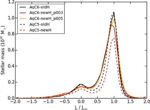
Stellar mass as a function of the circularity of stellar orbits at z = 0 for the following simulations: AqC6-oldH (black solid), AqC6-newH_p003 (red solid), AqC6-newH_p005 (orange solid), AqC5-oldH (black dashed), and AqC5-newH (red dashed).

Rotation curves for simulations AqC6-oldH (black solid line), AqC6-newH_p003 (red solid line), and AqC6-newH_p005 (orange solid line). Dashed lines refer to higher resolution simulations: AqC5-oldH (black) and AqC5-newH (red). All the curves describe the circular velocity due to the total mass inside a given radius.

Comparison between the baryon conversion efficiency from observations and from the simulated galaxies at z = 0. Curves show the stellar-to-halo mass relations derived by Guo et al. (2010, blue) and by Moster et al. (2010, purple), as in the right-hand panel of Figs 12 and 19. Symbols refer to simulations: AqC6-oldH (black filled circle), AqC6-newH_p003 (red filled circle), AqC6-newH_p005 (orange filled circle), AqC5-oldH (black filled triangle), and AqC5-newH (red filled triangle), respectively.
Fig. A2 shows SFRs as a function of the cosmic time (and of the redshift, too). SFRs of all the analysed simulations are comparable for z > 3. Then, if we focus on the AqC6 simulations, we see that the impact of the new hydrodynamic solver makes SFRs of AqC6-newH_p003 and AqC6-newH_p005 be lower than that of AqC6-oldH between 3 ≲ z ≲ 0.7. The main reason of this discrepancy lies in the presence of the time-step limiting particle wake-up scheme, as discussed for AqC5 runs in Section 5.2. AqC6-newH runs then overpredict the SFR until the cosmic time reaches ∼10 Gyr; from that moment on, the SFR of AqC6-newH_p003 starts to gently decline and matches the SFR of AqC6-oldH, while AqC6-newH_p005 keeps constantly larger than the prediction of AqC6-oldH (this is the actual reason why we prefer AqC6-newH_p003 rather than AqC6-newH_p005, though comparable). SFRs of AqC5-oldH and AqC6-oldH are relatively insensitive to mass resolution (see also M15); on the other hand, the variation of resolution is quite remarkable between AqC5-newH and AqC6-newH_p003 (and AqC6-newH_p005).
Fig. A3 describes the distribution of stellar mass as a function of the circularity of stellar orbits. All the galaxies are disc-dominated, with the hydrodynamic solver only slightly affecting the amount of stellar mass in both the bulge and the disc component. However, the different stellar mass in the disc component of AqC6-oldH and AqC6-newH_p003 (or AqC6-newH_p005, similarly) is not as pronounced as in the comparison between simulations AqC5-oldH and AqC5-newH. The effect of the resolution is much more apparent when using the new SPH scheme: a complete agreement between AqC6-newH_p003 and AqC5-newH is not reached even when the weak convergence is considered (Schaye et al. 2015). On the other hand, AqC6-oldH and AqC5-oldH show strong convergence with numerical resolution. B/T ratios for AqC6-oldH, AqC6-newH_p003, for AqC6-newH_p005, AqC5-oldH, and AqC5-newH are: 0.23, 0.25, 0.22, 0.23, and 0.30, respectively.
Fig. A4 shows results for the circular velocity profiles. Quite remarkably, none of the analysed profiles is centrally peaked, thus pinpointing that the adopted galactic outflow model is effective in preventing the formation of a too much centrally concentrated galaxy at both the resolutions. The different normalizations highlight the differences in the total stellar and gas mass that we obtain for the different tests. Values of the total stellar mass within the galactic radius Rgal are: 7.57 × 10¹⁰ M⊙ (Rgal = 24.00 kpc) for AqC6-oldH, 7.38 × 10¹⁰ M⊙ (Rgal = 24.19 kpc) for AqC6-newH_p003, 7.61 × 10¹⁰ M⊙ (Rgal = 24.24 kpc) for AqC6-newH_p005, 7.22 × 10¹⁰ M⊙ (Rgal = 23.86 kpc) for AqC5-oldH, and 4.74 × 10¹⁰ M⊙ (Rgal = 24.01 kpc) for AqC5-newH. Values of the gas mass within the galactic radius are: 1.85 × 10¹⁰ M⊙ for AqC6-oldH, 4.47 × 10¹⁰ M⊙ for AqC6-newH_p003, 4.37 × 10¹⁰ M⊙ for AqC6-newH_p005, 1.66 × 10¹⁰ M⊙ for AqC5-oldH, and 2.91 × 10¹⁰ M⊙ for AqC5-newH, at z = 0. We note that the difference in total stellar and gas mass between AqC5-oldH and AqC6-oldH are not as prominent as in the case AqC5-newH and AqC6-newH_p003 (or AqC6-newH_p005, similarly).
Fig. A5 shows the position of our simulations in the baryon conversion efficiency plot. We find that AqC5-newH has a lower baryon conversion efficiency than AqC5-oldH, while the baryon conversion efficiency is comparable when AqC6 simulations are analysed. Moreover, the lower the resolution is, the higher the stellar content of the simulated galaxy: this is independent of the adopted SPH scheme. However, such an effect is much more evident when the new SPH scheme is considered. For completeness, total baryonic masses within Rvir for the AqC6 runs are: 1.89 × 10¹¹ M⊙ for AqC6-oldH, 1.99 × 10¹¹ M⊙ for AqC6-newH_p003, and 2.06 × 10¹¹ M⊙ for AqC6-newH_p005, at z = 0.
Our general result is that properties of galaxies simulated at higher resolution are significantly more sensitive to the accuracy of the hydrodynamic solver.
APPENDIX B: TUNING THE PARAMETERS OF GALACTIC OUTFLOW MODELS
Feedback efficiency ffb,kin is the most delicate parameter of galactic outflow models. We report in this appendix our tests aimed at calibrating an optimal value of ffb,kin and its impact on the resulting properties of the simulated galaxies. In particular, we concentrate here on the effect of feedback efficiency in the FB1 and FB3 outflow models.
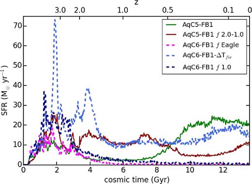
Evolution of the SFR for different simulations that adopt the FB1 outflow model.

Stellar mass as a function of the circularity of stellar orbits at z = 0 for different simulations adopting the FB1 galactic outflow model.
Equation (B1) for the feedback efficiency has been introduced according to the phenomenological approach (following Schaye et al. 2015) of using a higher feedback efficiency at high redshift. The above expression for ffb,kin is simpler than equation (11), and has been adopted to understand how different values for high-z and low-z feedback efficiency impact on SFR. By tuning the parameters |$f_{\rm fb,kin}^{\rm \,max}$| and |$f_{\rm fb,kin}^{\rm \,min}$|, it is possible to regulate high-z and low-z SFR.
Redshift z = 2 has been identified as the approximate epoch at which the bulge formation phase ends and the SF starts building up the disc component. After an exploration of the parameter space, we found that |$f_{\rm fb,kin}^{\rm \,max}=2.0$| and |$f_{\rm fb,kin}^{\rm \,min}=1.0$| are the most suitable parameters in reproducing a typical late-type galaxy SF history for our AqC5 simulations adopting the FB1 model. In particular, with such a choice, we are able to control low-redshift SF (see Fig. B1): ongoing SFR in the simulation AqC5-FB1f2.0-1.0 has been reduced by half with respect to AqC5-FB1.
Figs B1 and B2 describe the evolution of SFR and the distribution of the stellar mass as a function of the circularity of stellar orbits for the simulations adopting the galactic outflow model FB1, respectively. In these figures, we also include results from AqC6 resolution.
AqC6-FB1f Eagle is a simulation analogous to AqC5-FB1. At variance with the higher resolution simulation, AqC6-FB1f Eagle does not succeed to form a convincing disc galaxy, and it produces a spheroidal (see Fig. B2). AqC6-FB1-ΔTfix adopts the same feedback efficiency as the AqC6-FB1f Eagle (i.e. equation 11): in this simulation, we fix the temperature jump to the reference value of ΔT = 107.5 K (see Section 3.1). We find that this model is not able to prevent an excess of high-redshift SF, thus ending up with a disc galaxy having an unrealistically massive bulge.
The simulation AqC6-FB1f1.0 is analogous to AqC6-FB1fEagle, but it adopts a constant ffb,kin = 1.0. In this case, an SF burst at high redshift takes place (see Fig. B1). As a consequence, a prominent bulge is produced, with a resulting too small stellar disc due to the drastically reduced late-time SF. By adopting just one value for the feedback efficiency throughout the simulation, we do not succeed in producing a disc-dominated galaxy with this model (see Fig. B2). If the parameter ffb,kin is high enough to quench the high-redshift SF, then it depletes the amount of gas available for a subsequent phase of disc formation at low z. This is in agreement with Crain et al. (2015), who find that disc galaxies are characterized by a compact bulge and a too low low-redshift SFR if a constant stellar feedback efficiency is adopted.
Figs B1 and B2 also show that this galactic outflow model is resolution dependent (by considering AqC5-FB1 and AqC6-FB1fEagle). AqC5 simulations have an initial mass of gas particles that is ∼4.4 times smaller than the initial mass of baryonic particles in the reference Eagle simulation (Schaye et al. 2015), while AqC6 simulations have gas particles with a mass ∼3.7 times larger than that of particles of the same type in the reference Eagle simulation. This result suggests that this galactic outflow model promotes the formation of disc-dominated galaxies when a resolution at least higher than AqC6 simulations is considered (unless further re-calibration of parameters).
As for the FB3 galactic outflow model (Section 3.3), we here compare the evolution of SFRs and the circularity diagrams at z = 0 (Figs B3 and B4, respectively) for three simulations: AqC5-FB3_fk2.0, AqC5-FB3_fk0.5, and AqC5-FB3_fk0.25. For the sake of conciseness, we present results only for the variation of the feedback efficiency ffb,kin that spans the values 2.0, 0.5, and 0.25, respectively, while keeping the mass loading factor η = 3.0 fixed (see also Section 5.3.1).

Evolution of the SFR for different simulations that adopt the FB3 outflow model.
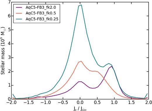
Stellar mass as a function of the circularity of stellar orbits at z = 0 for different simulations adopting the FB3 galactic outflow model.
We only vary the ffb,kin parameter for two reasons: first, it is the parameter to which the model is most sensitive. Second, Springel & Hernquist (2003), whose model this galactic outflow scheme is inspired, adopted ffb,kin = 0.25 for most of their simulations, even if they admitted that this feedback efficiency can assume values of order unity or even larger. Fig. B3 shows that a feedback efficiency larger than ffb,kin = 0.25 is needed in order to avoid a too high SFR, both at z > 1 – so as to quench SF in the bulge – and at low redshift. In fact, Fig. B4 demonstrates that simulated galaxies obtained for values of the feedback efficiency smaller than the reference value ffb,kin = 2 are mostly dominated by a dispersion-supported component (Jz/Jcirc = 0) rather than by a rotationally supported one (Jz/Jcirc = 1).
