


Abstract
Cosmic rays escaping the Galaxy exert a force on the interstellar medium directed away from the Galactic disc. If this force is larger than the gravitational pull due to the mass embedded in the Galaxy, then galactic winds may be launched. Such outflows may have important implications for the history of star formation of the host galaxy, and in turn affect in a crucial way the transport of cosmic rays, both due to advection with the wind and to the excitation of waves by the same cosmic rays, through streaming instability. The possibility to launch cosmic ray-induced winds and the properties of such winds depend on environmental conditions, such as the density and temperature of the plasma at the base of the wind and the gravitational potential, especially the one contributed by the dark matter halo. In this paper, we make a critical assessment of the possibility to launch cosmic ray-induced winds for a Milky Way-like galaxy and how the properties of the wind depend upon the conditions at the base of the wind. Special attention is devoted to the implications of different conditions for wind launching on the spectrum of cosmic rays observed at different locations in the disc of the galaxy. We also comment on how cosmic ray-induced winds compare with recent observations of Oxygen absorption lines in quasar spectra and emission lines from blank sky, as measured by XMM–Newton/EPIC-MOS.
1 INTRODUCTION
Galactic winds have been observed in many galaxies (see e.g. Veilleux, Cecil & Bland-Hawthorn 2005; Martin et al. 2012; King & Pounds 2015) and constitute an important feedback process to the evolution of galaxies. In fact, by removing gas from the galactic disc, galactic winds regulate the star formation rate (see e.g. Crain et al. 2007) and pollute galactic haloes and intergalactic space with hot plasma and metals, thus affecting the chemical composition, the temperature and the degree of ionization of the interstellar medium (ISM) and of the intergalactic medium (IGM, see e.g. Miller & Bregman 2015). Moreover, the expelled material may contain an appreciable fraction of the number of baryons in the Universe (see e.g. Kalberla & Dedes 2008; Miller & Bregman 2015) and may contribute to solving the problem of missing baryons in the local Universe (see e.g. Anderson & Bregman 2010). Although observations of the Milky Way have not yet led to conclusive evidence of the existence of a Galactic wind, hot dilute gas, possibly connected with such winds, have been detected through the continuous emission in the X-ray band (Breitschwerdt & Schmutzler 1994, 1999; Everett et al. 2008) and through Oxygen absorption lines (OVII and OVIII lines) in the spectrum of distant quasars (Miller & Bregman 2015). The features of such lines are compatible with a halo with a mass of ∼ 1010 M⊙, an extension of ∼100 kpc, a temperature in the range 106–107 K and an average metallicity of Z ∼ 0.2–0.3. In particular, the latter data imply that the gas in the halo comes from the Galaxy and not from intergalactic space (Miller & Bregman 2015). Moreover, the recent observation of the so-called Fermi Bubbles may be associated to recent bursts near the Galactic Centre region (see Cheng et al. 2011; Zubovas, King & Nayakshin 2011) or to past starburst activities (see Lacki 2014).
Galactic winds may be (1) thermally driven, namely generated by the heating of the ISM due to supernova (SN) explosions (see e.g. Chevalier & Clegg 1985) or by accretion on to the supermassive black holes in the centre of active galactic nucleus (see e.g. King & Pounds 2015); (2) radiation pressure-driven (see e.g. Scoville 2003; Murray, Quataert & Thompson 2005); (3) cosmic ray (CR)-driven, namely due to the pressure exerted by escaping CRs on the ISM (see e.g. Ipavich 1975; Breitschwerdt, McKenzie & Voelk 1991; Uhlig et al. 2012). The first two mechanisms are likely to take place in starburst galaxies and galaxies with active nuclei.
In the Milky Way, the thermal and radiation pressure gradients are expected to be too small (except perhaps for the Galactic Centre region) to drive outflows. However, CRs escaping from the Galaxy lead to a gradient in the CR density with several implications. First, the CR pressure gradient exerts a force, −∇Pc, on the background plasma directed away from the disc and opposite to the Galactic gravitational force (due to both baryonic and dark matter, DM). If this force is larger than the gravitational pull it may launch a wind. Second, the CR density gradient can excite Alfvén waves, due to CR streaming instability (Kulsrud & Cesarsky 1971; Skilling 1975), which move in the direction of the decreasing CR density. Such waves affect the scattering properties of CRs, namely their diffusive transport. Third, winds and the waves that propagate inside the outgoing plasma, advect CRs and contribute to change the spectrum of CRs as observed in the Galaxy.
CRs have been widely recognized as an appealing way to launch winds in our Galaxy and the hydrodynamics of CR-driven winds has been extensively studied in stationary one-dimensional calculations (see e.g. Ipavich 1975; Breitschwerdt et al. 1991; Everett et al. 2008; Zirakashvili et al. 1996), in time-dependent calculations (Dorfi & Breitschwerdt 2012), in hydrodynamical simulations (see Uhlig et al. 2012; Booth et al. 2013; Salem & Bryan 2014) and in magnetohydrodynamic simulations (see Girichidis et al. 2016; Ruszkowski, Yang & Zweibel 2016). The paper by Breitschwerdt et al. (1991) represented a crucial step forward in the investigation of CR-driven Galactic winds: their computation techniques have been adopted by much of the subsequent work on the subject.
In all this bulk of work, no matter the level of refinement, only the hydrodynamics of CR-driven winds was addressed, while no information was retained on the CR spectrum in such winds. On the other hand, the CR spectrum represents a crucial observable that we can use in order to constraint wind models, hence its prediction is essential. Recently, our group (Recchia, Blasi & Morlino 2016, hereafter Paper I) presented an extensive study of the problem of the CR transport in a CR-driven wind. We developed a semi-analytical method which allows to compute self-consistently the hydrodynamical properties of CR-driven winds and the corresponding CR distribution function in the presence of self-generated Alfvén waves. In our approach, the hydrodynamics of the wind is calculated following the one-dimensional stationary model developed by Breitschwerdt et al. (1991) and the CR transport is due to scattering of CRs on the self-generated turbulence and to the CR advection with such waves and with the wind. Both the flow and the CR transport only occur along the magnetic field lines and the flow geometry is pre-assigned. The CR diffusion coefficient is calculated from the spectrum of waves excited by streaming instability and locally damped through non-linear Landau damping (NLLD). The importance of CRs for wind launching was confirmed by our work, although we found that in general, the CR spectrum in the presence of winds launched in the vicinity of the Sun is not in agreement with observations. This is mainly due to the fact that CR advection in such winds is strong, leading to spectra at low energies (below ∼200 GeV) which are harder than the observed spectrum. At high energy (above ∼200 GeV), instead, the wind expansion together with the steep energy dependence of the self-generated diffusion coefficient, leads to spectra that are steeper than the observed spectrum. However, these conclusions strongly depend, at low energy, on the wind launching parameters and, at high energy, on the physical conditions in the near-disc region, in particular on the amount of neutral gas in such region and on its volume filling factor. For instance, we showed that at high energy the CR spectrum is very sensitive to the diffusion properties of the near-disc region (≲ 1 kpc) where the presence of a pre-existing turbulence would lead to a spectral hardening in the high-energy part of the spectrum (see also Aloisio, Blasi & Serpico 2015), in agreement with recent observations of the proton and helium spectrum (see Adriani et al. 2011; Aguilar et al. 2015).
In this paper, we use the calculations developed in Paper I and we study the possibility to launch winds, the dependence of the wind properties on environmental parameters and the implications of such dependencies for the spectrum of CRs observed at the Sun position. Special attention is devoted to investigating the wind properties as functions of the ISM properties (gas density and temperature, Galactic magnetic field), CR pressure, flow geometry and on the Galactic gravitational potential.
The spatial dependence of these quantities in the Galaxy is constrained by observations (see e.g. Ferrière 2001; Cox 2005; Wolfire et al. 2003; Miller & Bregman 2015). In particular, the observation of the Oxygen absorption lines in the spectrum of distant quasars analysed by Miller & Bregman (2015) suggests the presence of a large Galactic halo, presumably due to a Galactic wind, and provides us with indications on the gas mass distribution and temperature of such halo, and consequently on the flow geometry. Moreover, the baryonic and DM content of the Milky Way and the corresponding gravitational potential can be constrained by analysing the dynamics of stars and gas (see e.g. Bertone, Hooper & Silk 2005; Sofue 2012; Nesti & Salucci 2013). We discuss how our results change by adopting different distributions of Galactic DM and compare them with the halo structure deduced by Miller & Bregman (2015).
The paper is organized as follows: in Section 2, we describe our wind model and we briefly summarize the method used to solve the hydrodynamic wind equations and the CR transport equation, as illustrated in Paper I. In Section 3, we describe the model used for the gravitational potential of the Galaxy, including several DM halo models. In Section 4, we summarize the main properties of the ISM as deduced from observations and their relevance for the models of CR-driven winds. In Section 5, we discuss in detail the dependence of the wind properties on the parameters of the problem, as well as on the geometry of the outflow and the Galactic gravitational potential. Finally, in Section 6, we illustrate the implications of CR-driven winds launched at the position of the Sun on the spectrum of CRs.
2 THE WIND MODEL
The dynamics of a CR-driven wind in the stationary regime is described by the system of hydrodynamic equations for the wind (i.e. the equations of mass, momentum and energy conservation) and by the kinetic transport equation for CRs. The hydrodynamic wind equations have been written down and discussed in detail by Breitschwerdt et al. (1991). A method to calculate the combined solution of the hydrodynamical equations for the wind and the transport equation of CRs has been recently developed in Paper I. This method allows one to determine at the same time the wind structure and the related CR spatial and momentum distribution. Here, we briefly summarize the equations and the main features of the wind model.
Two important quantities appear in these equations: the generalized sound speed c* and the effective adiabatic index for CRs, γeff. Looking at the definition of |$c_{*}^2$|, equation (6), one can recognize the sum of the sound speed term (square root of γgPg/ρ) and of a ‘CR sound speed' term (the term γeffPc/ρ is formally identical to the square root of the sound speed) which depends on the Alfvénic Mach number u/vA. Note that the term −(γg − 1)vA/u is due to the non-adiabatic gas heating induced by wave damping in equation (4). The importance of c* resides in the fact that u = c* is the condition for the flow to become sonic but also is a critical point for the wind equation (3). The effective adiabatic index for CRs, γeff, takes into account the CR diffusivity in the hydrodynamic equations (see also Zirakashvili et al. 1996). In general, γeff is a function of z, however, it has been verified that in general (including in the cases presented here) γeff shows a weak dependence on z and we can safely treat it as a constant. Typical values of γeff ∼ 1.1–1.2, while γc ∼ 4/3. Breitschwerdt et al. (1991) also introduced the generalized sound speed c* but with two important differences compared with the calculation discussed here. First, they neglected the CR diffusion by assuming that |$\overline{D}=0$| so that in their calculation γc appears instead of γeff. Neglecting diffusion is not a good approximation, at least not at all distances z from the disc. Second, Breitschwerdt et al. (1991) did not take wave damping into account and retained the wave pressure in the hydrodynamic equations. Without damping, the growth of waves due to CR streaming can in fact lead to a wave pressure which is comparable with the CR pressure. For this reason, instead of having the term −(γg − 1)vA/u in the definition of |$c_{*}^2$|, they have a ‘wave sound speed' term which takes into account the effect of the wave pressure.
Following Paper I, the hydrodynamic equations for the wind and the CR transport equation are solved together following at iteration scheme. For a given set of input parameters at the wind base z0 (namely the gas density ρ0, the gas temperature T0, the magnetic field strength B0 and the CR pressure Pc0), for each iteration, we determine the velocity u0 at the base of the wind, for which the flow experiences a smooth transition from the subsonic to the supersonic regime. Given u0, both the mass and energy flux of the wind are fixed, and it is possible to compute all the hydrodynamic quantities (gas density and pressure, wind velocity and CR pressure) as functions of the distance from the Galactic disc. For each iteration, the transport equation (8) is solved for the CR distribution function f(z, p) and the diffusion coefficient D(p, z). The iteration is then repeated until convergence is reached within a given accuracy.
3 THE GALACTIC GRAVITATIONAL POTENTIAL
The mass distribution of the Milky Way, and of other galaxies as well, is mainly inferred from analyses of the dynamics of stars and gas, namely by studying kinematic data such as rotation velocities, velocity dispersions and motion of satellite galaxies. Current models for the mass distribution of the Galaxy include a central bulge, a stellar and gas disc and a DM halo (see e.g. Irrgang et al. 2013).
For the DM mass distribution we considered three models, namely the Navarro–Frenk–White (NFW, Navarro, Frenk & White 1996), the Burkert (BUR, Burkert 1995) and the Einasto (EIN, Retana-Montenegro et al. 2012) profiles:
NFW (Navarro et al. 1996):
the density profile is of the formwhere x = r/rc and rc is the scale radius of the distribution. For the two quantities ρ0 and rc, we considered both the values given for the Milky Way by Sofue (2012) (ρ0 = 1.06 × 10⁷ M⊙ kpc−3; rc = 12.0 kpc) and by Nesti & Salucci (2013) (ρ0 = 1.3 × 10⁷ M⊙ kpc−3; rc = 16.0 kpc). We refer to the two sets of parameters as NFW–Sofue and NFW–Salucci, respectively. The DM halo is assumed to extend out to a maximum distance that equals the virial radius, which corresponds to rvir ≈ 240 kpc for NFW–Sofue and rvir ≈ 320 kpc for NFW–Salucci.(18)\begin{equation} \rho _{\rm NFW} = \frac{\rho _{0}}{x(1+x)^{2}}, \end{equation}BUR (Burkert 1995):
the density profile is of the formwhere x = r/rc and rc is the core radius. For the two quantities ρ0 and rc, we considered the values given for the Milky Way by Nesti & Salucci (2013) (ρ0 = 4.13 × 10⁷ M⊙ kpc−3; rc = 9.3 kpc). The virial radius for this model is rvir ≈ 300 kpc.(19)\begin{equation} \rho _{\rm BUR} = \frac{\rho _{0}}{(1+x)(1+x^2)}, \end{equation}EIN (Retana-Montenegro et al. 2012):
the density profile is of the formwhere x = r/rc. For the three quantities ρ0, rc and α, we considered the values given for the Milky Way by Bernal & Palomares-Ruiz (2012) (ρ0 = 3.5 × 10¹¹ M⊙ kpc−3, rc = 6.7 × 10⁻⁶ kpc and α = 0.17).(20)\begin{equation} \rho _{\rm EIN} = \rho _0 \exp (-x^{\alpha }), \end{equation}
These halo models predict a DM density at the Sun position in the range 0.2–0.4 GeV cm−3, in agreement with most of the current literature (see Salucci et al. 2010 for a discussion on the local DM density).
A comparison between the gravitational acceleration produced by different DM models at the solar galactocentric distance R = R⊙ and as a function of the Galactic altitude is shown in Fig. 1 where also the contribution due to the disk and to the bulge are reported. One can see that the BUR and the EIN profiles are quite similar in magnitude below z ∼ 50 kpc and that the EIN profile becomes systematically larger than the BUR profile above z ∼ 50 kpc. On the other hand, the NFW profile shows large differences in magnitude, compared to the other two profiles, below z ∼ 30–40 kpc. Since these profiles predict a similar DM density at the Sun, this is due to the different functional dependence on x = r/rc and to the different values of the scale radius rc.
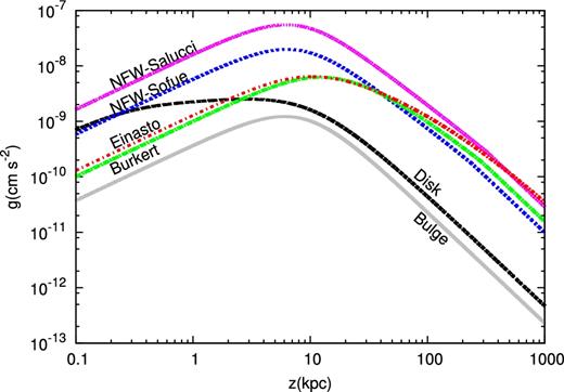
Galactic gravitational acceleration as function of the distance from the galactic plane, z, at the Sun position produced by different DM profiles. The contribution due to the and the bulge are also shown.
4 FIDUCIAL VALUES FOR THE ENVIRONMENTAL PARAMETERS
The ISM is a rich environment in which several components, distinguished by the level of ionization and temperature, coexist and interact: molecular and atomic neutral gas, warm and hot ionized gas, interstellar magnetic field and CRs. In the cooler, denser regions of the ISM, matter is primarily in molecular form and can reach densities as high as 106 cm−3. On the other hand, in the diffuse regions of the ISM, matter is mainly ionized and can reach densities as low as 10−4 cm−3. In addition, the colder and denser phases of the ISM are mainly confined in the Galactic and have filling factor of order ∼1–5 per cent, much smaller than the dilute hot gas filling factor, which is of order 30–70 per cent. A detailed study of the gas components of the ISM has been carried out by several authors (see e.g. Cox 2005; Wolfire et al. 2003), while a comprehensive review of the present knowledge of the ISM can be found in Ferrière (2001). In Table 1, we summarize the main properties of the gas components of the ISM in the vicinity of the Sun as reported by Ferrière (2001).
Components of the ISM and their properties in the vicinity of the Sun (see Ferrière 2001).
| Component | Temperature | Density | Scaleheight |
|---|---|---|---|
| (K) | (cm−3) | (kpc) | |
| Molecular | 10–20 | 102–106 | ∼0.1 |
| Cold atomic | 50–100 | 20–50 | ∼0.1–0.4 |
| Warm atomic | 6000–10 000 | 0.2–0.5 | ∼0.1–0.4 |
| Warm ionized | 8000 | 0.2–0.5 | ∼ 1 |
| Hot ionized | ∼106 | ∼ 0.006 | >1 |
The Galactic magnetic field shows a rich structure in which at least a component, which follows the spiral arms, and an out of component can be found (see Jansson & Farrar 2012). The regular field strength changes with the Galactocentric distance. An estimation of the magnetic field strength in the vicinity of the Sun is reported for instance in Jansson & Farrar (2012), which quote the value ∼ 1-2 μG for the component and ∼ 1 μG for the out of component. Ferrière (2001) quote a value B⊙ ∼ 1.5 μG, while Cox (2005) suggest a value of ∼ 3-5 μG (which includes all field components). Here, we are mainly interested in the out of component.
This halo model implies a gas density of 3–6 × 10⁻³ cm−3 in the vicinity of the Sun, a density scaling with z that reads n(z) ∼ z−1.5 and a halo mass of M( < 50 kpc) = (3.8 ± 0.3) × 109 M⊙ and M( < 250 kpc) = (4.3 ± 0.8) × 1010 M⊙. Note that such halo mass would account for ≲ 50 per cent of the Milky Way missing baryons.
All these pieces of information allow us to define reasonable fiducial values for the input parameters of our wind problem (see Table 2 for a summary): we are interested in the hot dilute phase of the ISM, for which we adopt a density 3–6 × 10⁻³ cm−3 and a temperature 1–3 × 10⁶ K, and in the out of regular magnetic field for which we retain a field strength 1-2μG.
Fiducial values for the wind input parameters at the Sun position.
| Parameter | Fiducial range |
|---|---|
| Area-α | 1.5–2.0 |
| Area-Zb | 5–15 kpc |
| Gas density | 3–6 × 10⁻³ cm−3 |
| Gas temperature | 1–3 × 10⁶ K |
| Regular B | 1-2 μG |
| CR pressure | 4 × 10⁻¹³ erg cm−3 |
| Parameter | Fiducial range |
|---|---|
| Area-α | 1.5–2.0 |
| Area-Zb | 5–15 kpc |
| Gas density | 3–6 × 10⁻³ cm−3 |
| Gas temperature | 1–3 × 10⁶ K |
| Regular B | 1-2 μG |
| CR pressure | 4 × 10⁻¹³ erg cm−3 |
The pressure in the form of CR protons measured at Earth is ∼4 × 10⁻¹³ erg cm−3.
Finally, Breitschwerdt et al. (1991), Everett et al. (2008) and Paper I assumed that the flux tube opens up spherically, namely α = 2 in equation (16), while the results of Miller & Bregman (2015) suggest α ∼ 1.5. As for the area length-scale Zb, Breitschwerdt et al. (1991) and Paper I adopted the value 15 kpc, while Everett et al. (2008) treated Zb as a fitting parameter and allowed it to vary around ∼5 kpc. Here, we consider α ∼ 1.5–2 and Zb ∼ 5–15 kpc.
5 DEPENDENCE OF THE WIND PROPERTIES ON THE GALACTIC ENVIRONMENT
In this section, we present a purely hydrodynamical analysis of Galactic winds, launched at the Sun position, focusing on how the wind's properties are affected when changing the environmental parameters within the range allowed by observations, as summarized in Section4. In Section 5.3, we briefly discuss the role of radiative cooling while we describe the implications for the CR spectrum in such winds in Section 6.
The topology of the solutions of the hydrodynamic equations (1)–(7) depends on the nature of the critical points of the wind equation (3) (see Breitschwerdt et al. 1991, Paper I), i.e. of the points in which the velocity derivative has zero numerator |$(c_{*}^2= \frac{{\rm d}\Phi }{{\rm d}z}/\frac{1}{A} \frac{{\rm d}A}{{\rm d}z})$| and/or zero denominator (|$u^2=c_{*}^2$|). The point for which both the numerator and the denominator vanish is the critical (sonic) point, and it corresponds to the location where the flow velocity equals the compound sound speed, i.e. u = c*. The solution relevant for our problem is the one with velocity that starts subsonic at the wind base z0, increases with z, goes through the critical point where it becomes supersonic and keeps increasing (wind acceleration). The wind launching velocity u0 for this solution is found by imposing crossing through the critical point. For launching velocities smaller than u0, the flow remains subsonic everywhere and there is a point in which the numerator of equation (3) vanishes. Such solutions are called ‘breezes'. For launching velocities larger than u0 but still subsonic, there is a point in which the denominator of equation (3) vanishes and the corresponding solutions are unphysical.
where M = u/c* is the Mach number and |$\mathfrak {a}(z) \equiv \frac{1}{A}\frac{{\rm d}A}{{\rm d}z}$| for the De Laval nozzle. In Fig. 2, the scheme of a De Laval nozzle is shown. Note that the nozzle has a converging and a diverging section. If we look at equation (26), we see that this converging–diverging duct makes a smooth subsonic–supersonic transition possible: the flow starts subsonic in the converging duct (|$\mathfrak {a}(z) < 0$| and M < 1), becomes sonic at the throat (|$\mathfrak {a}(z) = 0$| and M = 1) and is accelerated to supersonic speed in the diverging duct (|$\mathfrak {a}(z) > 0$| and M > 1). In such configuration, it is possible to constantly accelerate the flow along the nozzle (du/dz remains positive). The sonic transition is only possible at the nozzle throat (choking), where |$\mathfrak {a}=0$|.
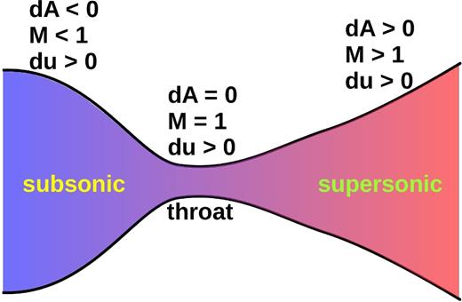
Scheme of a De Laval nozzle: the flow is smoothly accelerated (du/dz > 0 in all the duct) from the subsonic (M < 1) to the supersonic regime (M > 1). The flow is subsonic in the converging section (dA/dz < 0), becomes sonic at the throat (dA/dz = 0, M = 1) and continues to accelerate to supersonic speed in the diverging section (dA/dz > 0).
The numerator of the CR-driven wind equation (25) presents an ‘effective area' term given by |$a(z) -\frac{g(z)}{c^{*2}}$|, which plays the same role of |$\mathfrak {a}(z)$| in the De Laval equation. Thus, in order to have a smooth subsonic–supersonic transition, the effective area must have the same convergent–divergent behaviour of the De Laval nozzle:
u2 < c*2 (subsonic regime)
the gravitational term g(z) must dominate in the numerator in order to have du/dz > 0. Thus, g(z) is a ‘converging duct' term,
u2 > c*2 (supersonic regime)
the area term a(z) must dominate in the numerator in order to have du/dz > 0. Thus, a(z) is a ‘diverging duct' term.
It is clear from this analysis that if a(z) = 0, i.e. if the flux-tube area is constant, a wind solution cannot be achieved. Similarly, if the a(z) > 0, namely the flow only expands (as in our wind model), the gravitational term |$\frac{g(z)}{c^{*2}}$| allows for the presence of a stationary wind solution.
Finally, the passage through the critical point (choking condition for the De Laval nozzle) fixes the wind launching velocity u0. Because all other magnitudes in equations (22) and (23) are assigned at the wind base, this also fixes the mass and energy flux of the wind.
In order to carry out an analysis of the effects of the input parameters on the flow, it is helpful to define a reference model to which all other cases can be compared. Because we are considering winds launched at the Sun position, we define our reference case starting from observations and we choose: z0 = 100 pc for the wind base (winds launched near the Galactic), n0 = 6 × 10⁻³ cm−3 for the gas density, T0 = 2 × 10⁶ K for the gas temperature, Pc0 = 4 × 10⁻¹³ erg cm−3 for the CR pressure, B0 = 1 μG for the magnetic field, Zb = 15 kpc and α = 2.0 for the area parameters and NFW–Sofue for the DM profile. The latter choice is motivated by the fact that the NFW profile is one of the most commonly used models for DM haloes.
In Figs 3(a)–(c), we reported the spatial profile of the wind related quantities for the reference case, while the various components of the Galactic gravitational acceleration have been previously shown in Fig. 1. Note that, unlike the bulge and components, which die off at ∼10 kpc, the DM contribution to the acceleration remains important out to the virial radius (∼ 240 kpc for the NFW–Sofue).
For the reference case, at the wind base the flow is subsonic and sub-Alfvénic and most of the work on the gas is due to the thermal pressure, which is four times larger than the CR pressure. CRs contribute to push the gas, however a considerable fraction of their energy is used to generate Alfvén waves, which are quickly damped and heat the gas. This can be seen in Fig. 3(b), where it is shown that the gas temperature increases up to ∼10 kpc and then decreases in z much slower than the gas density. Because of the CR-induced gas heating, also the gas pressure falls off in z slower than it would in the absence of wave damping. Nevertheless, the gas pressure decreases with height much faster than the CR pressure, and at ∼20 kpc the CR pressure starts to dominate over the gas pressure. This is due to the fact that CRs have a smaller adiabatic index compared to the gas (γc ∼ 4/3 and γg = 5/3), which has important consequences on the relative contribution of the thermal and CR pressure to the wind launching. For instance, while the thermal pressure is more efficient in accelerating the gas near the wind base, the CR pressure is able to push the gas also at large z, often making an outflow possible where the thermal pressure alone would have failed (see Ipavich 1975; Breitschwerdt et al. 1991; Everett et al. 2008).
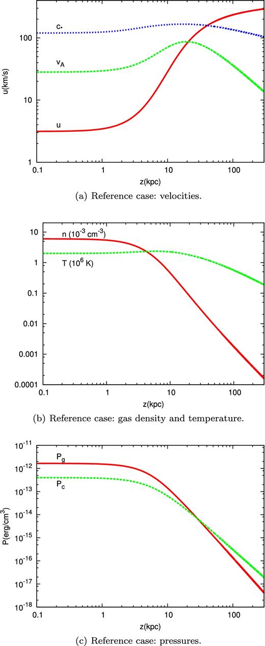
Reference case: (a) wind, Alfvén and compound sound speeds; (b) gas density and temperature; (c) gas and CR pressures. The input parameters are: z0 = 100 pc, n0 = 6 × 10⁻³ cm−3, T0 = 2 × 10⁶ K, Pc0 = 4 × 10⁻¹³ erg cm−3, B0 = 1 μG, Zb = 15 kpc, α = 2.0 and the NFW–Sofue DM profile.
Having defined a reference set of parameters, below we study the dependence of the outflow properties on the input parameters at the wind base. In Section 5.1, we focus on the effect of changes of the gas density, gas temperature and CR pressure, while the analysis of the dependence on the area parameters is reported in Section 5.2.
5.1 Effect of the gas density and temperature and of the cosmic ray pressure
In order to emphasize the dependence of the results on the input parameters, here we also include in our analysis parameters' values that are not strictly compatible with observations at the position of the Sun (discussed in Section 4).
In Tables 3 –5, we report the launching velocity u0, the position of the sonic point zc and the terminal velocity uf, for different values of the gas density (Table 3), gas temperature (Table 4) and CR pressure (Table 5), as compared with the reference case of Fig. 3 (indicated by the superscript ‘R').
Dependence of the wind properties on the gas density. The gas temperature (2 × 10⁶ K) and CR pressure (|$4\times 10^{-13} \rm\, erg\, cm^{-3}$|) are fixed. |$\dot{m}$| is the mass-loss rate of the wind.
| Gas density | u0 | zc | uf | |$\dot{m}$| |
|---|---|---|---|---|
| |$n_0^{\rm R} = 6\times 10^{-3}$| | 4.7 × 10⁻⁴ | |||
| (cm− 3) | (km s−1) | (kpc) | (km s−1) | |$(\rm M_{{\odot }}\, kpc^{-2}\, \rm yr^{-1})$| |
| 0.2 | 39.7 | 18.9 | 595 | 2.5 |
| 0.5 | 10.7 | 30.9 | 428 | 1.7 |
| 1.0 | 3.1 | 40.6 | 403.7 | 1.0 |
| 3.0 | 0.8 | 72.2 | 296 | 0.73 |
| 6.0 | 0.3 | 96.5 | 269 | 0.53 |
Dependence of the wind properties on the gas temperature. The gas density (6 × 10− 3 cm− 3) and CR pressure (4 × 10− 13 erg cm− 3) are fixed.
| Gas temperature | u0 | zc | uf | |$\dot{m}$| |
|---|---|---|---|---|
| |$T_0^{\rm R} = 2\times 10^6$| | 4.7 × 10⁻⁴ | |||
| (K) | (km s−1) | (kpc) | (km s−1) | |$(\rm M_{{\odot }}\, kpc^{-2}\, \rm yr^{-1})$| |
| 0.5 | 3.09 | 34.3 | 419 | 0.98 |
| 1.0 | 3.1 | 40.6 | 403.7 | 1 |
| 2.0 | 6.9 | 104.9 | 243 | 2.2 |
| 3.0 | 17.5 | 367.6 | 152.4 | 5.6 |
| 4.0 | 182 | 13.32 | 263 | 58 |
| 5.0 | 280 | 7.8 | 441.3 | 89 |
| 6.0 | 362 | 4.8 | 573.5 | 116 |
Dependence of the wind properties on the CR pressure. The gas density (6 × 10− 3 cm− 3) and temperature (2 × 10⁶ K) are fixed.
| CR pressure | u0 | zc | uf | |$\dot{m}$| |
|---|---|---|---|---|
| |$P_{{\rm c}0}^{\rm R} = 4\times 10^{-13}$| | 4.7 × 10⁻⁴ | |||
| (erg cm− 3) | (km s−1) | (kpc) | (km s−1) | |$(\rm M_{{\odot }}\, kpc^{-2}\, \rm yr^{-1})$| |
| 0.2 | 0.72 | 64.1 | 339 | 0.2 |
| 0.5 | 1.84 | 51.2 | 351 | 0.6 |
| 1.0 | 3.1 | 40.6 | 403.7 | 1 |
| 2.0 | 8.6 | 36.9 | 376.5 | 2.8 |
| 3.0 | 14.5 | 32.6 | 394 | 4.6 |
| 4.0 | 21.8 | 29.2 | 415 | 7.0 |
| 5.0 | 30.7 | 26.2 | 439.6 | 9.8 |
| 6.0 | 41.1 | 23.6 | 573.5 | 13 |
Some basic considerations can be put forward based on purely energetic grounds. Consider for instance what happens at fixed gas density and CR pressure values as in Table 4: for temperatures below |${\sim } 0.4\, T_0^{\rm R}$|, it is impossible to launch a wind simply because the energy available is too small. In the opposite limit, for instance for temperature |${\gtrsim } 7\, T_0^{\rm R}$|, the gas is simply too hot and the outflow resembles more an evaporation process, which in reality would result in a non-stationary outflow that cannot be described using our formalism (see also Everett et al. 2008).
At fixed gas temperature and CR pressure, an increase in the gas density leads to a decrease of both the launching velocity u0 and the terminal velocity uf (see Table 3). This is not surprising, since a larger mass load makes more difficult for the pressure forces to launch a wind. Note that the decrease of u0 with increasing density is fast enough to drive down the mass-loss rate of the wind (which is proportional to n0 u0) despite the increasing density (see Table 3).
The behaviour of the terminal velocity with the gas temperature and the CR pressure is a bit more complicated being non-monotonic. In Tables 4 and 5, we can see that, when increasing both Pc0 and ρ0, the terminal velocity in general does not increase. Keeping the gas density and the CR pressure at the reference values and increasing the temperature from |$0.5\,T_0^{\rm R}$| to |$3\, T_0^{\rm R}$|, uf decreases by a factor ∼3, while from |$3\,T_0^{\rm R}$| to |$6\, T_0^{\rm R}$|, it increases by factor of ∼4. Similarly, keeping the gas density and temperature at the reference values and increasing the CR pressure from |$0.2\,P_{{\rm c}0}^{\rm R}$| to |$P_{{\rm c}0}^{\rm R}$|, uf increases. It decreases when the CR pressure goes from |$P_{{\rm c}0}^{\rm R}$| to |$2\, P_{{\rm c}0}^{\rm R}$|, and finally increases for CR pressure from |$2\, P_{{\rm c}0}^{\rm R}$| to |$6\, P_{{\rm c}0}^{\rm R}$|.
The location of the sonic point is closer to the Galactic for smaller gas density and for larger gas temperature and CR pressures. This is due to the fact that in all three cases the gas is accelerated more easily and in general reaches the sonic point at smaller z.
It is also worth stressing the role played by wave damping. Breitschwerdt et al. (1991) did not study the effect of wave damping in detail and the paper mainly focused on a model where Alfvén waves, produced through CR streaming instability, are not damped and can grow indefinitely. In such a model, the parameter space for the wind launching was much larger than in the case where wave damping is included, resulting in the possibility to easily launch winds also at relatively low temperatures and high gas densities. In the presence of wave damping, the parameter space is reduced, mainly due to two factors. First, if waves are not damped, their pressure contribution, which grows to reach more or less the same magnitude as the CR pressure, can significantly help in pushing the gas. Second when the waves are damped, the heat input from wave damping increases the temperature (and thus the gas pressure) along z, which results in a smaller gas pressure gradient, i.e. a smaller force acting on to the wind. If the contribution of wave damping is too intense, the gas heating can be so important so as to make the gas pressure increase with z, thus creating a stall in the outflow. In this situation, the wind formation is prevented (see Everett et al. 2008).
We conclude this overview with a discussion of the mass-loss rate of the Galaxy due to winds. In Tables 3–5, we report the mass-loss rate per unit area for different values of the launching parameters of the wind. If we assume that such mass-loss rate per unit area is the same as in the whole Galactic and we consider input parameters compatible with the halo observations, we obtain a mass-loss rate roughly in the range ∼ 0.5-1.5 M⊙ yr− 1. Such values of the mass-loss rate are of the same order of magnitude of the Galactic star formation rate (∼M⊙ yr−1; see e.g. Robitaille & Whitney 2010), which means that CR-driven Galactic winds may play an important role in the evolution of the Milky Way.
It is also worth stressing that, if we consider the mass-loss rate per unit area at the Solar circle corresponding to the reference case reported above, namely 4.7 × 10− 4 M⊙ kpc− 2 yr, and we assume a column density for the of 2 × 1020 cm− 2 (in one direction from the mid-plane), such wind would deplete the gas in ∼3 Gyr. On the other hand, one should keep in mind that mass is also injected in the through SN explosions and stellar winds at roughly the same rate, so as to avoid the depletion mentioned above. Moreover, it is worth recalling that some gas removal is in fact required by models of star formation Crain et al. (2007), and winds are often invoked to provide such depletion.
5.2 Effect of the flux-tube geometry
Here, we analyse the impact of the flux-tube geometry through the variation of the two parameters α and Zb of equation (16), keeping the gas density, temperature and CR pressure to the reference values of Fig. 3 and using the NFW–Sofue DM profile. The ‘mushroom' type geometry of equation (16) reflects what we would intuitively expect for outflows from galaxies: the flow proceeds in nearly cylindrical symmetry up to about a distance Zb from the galactic and then opens up in a nearly spherical way. Of course, in a full treatment of the CR-driven wind problem, the flow geometry should be calculated self-consistently by accounting for the large-scale magnetic field. However, such study is beyond the scope of the present work, hence we retain the geometry described by equation (16) and we study how the wind properties get modified when Zb and α are changed.
The flux-tube geometry directly affects the acceleration of the outflow, as well as the gas density (see equations 22 and 24) and consequently the pressure gradients (see equations 4 and 5). Thus, it is not surprising that the shape chosen for the function A(z) has important implications for the wind properties. In what follows, we first discuss the effect produced by changing the length-scale, Zb, and then the effect of changing the exponent α:
5.2.1 Effect of changing the length-scale Zb
We fix α = 2.0 and we change Zb in the range 5–20 kpc, stepped by 2.5 kpc. In Table 6, we show the wind launching velocity u0, the wind terminal velocity uf and the location of the sonic point zc as functions of Zb, while in Fig. 4, we report the wind profile (relevant velocities, densities, temperature and pressures) for the two extremal cases Zb = 5 and 20 kpc.
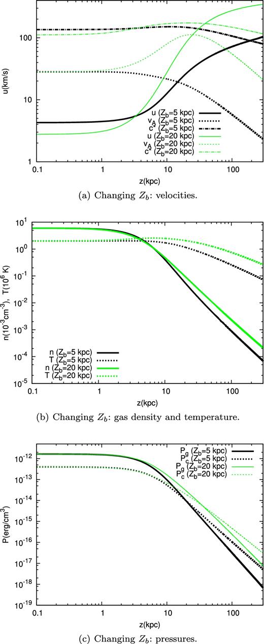
Comparison of wind profiles in case of changing the flux-tube geometry. Two cases are shown, Zb = 5 and 20 kpc, while the value of α is fixed to 2. The different plots are: (a) wind, Alfvén and compound sound speed; (b) gas density and temperature; (c) gas and CR pressures.
Dependence of the wind properties on the area length-scale Zb. The gas density (3 × 10− 3 cm− 3), gas temperature (2 × 10⁶ K) and CR pressure (4 × 10− 13 erg cm− 3) are fixed. α = 2.0.
| Zb (kpc) | u0 (km s−1) | zc (kpc) | uf (km s−1) |
|---|---|---|---|
| 5.0 | 4.3 | 189.9 | 218.4 |
| 7.5 | 4.0 | 89.7 | 266.0 |
| 10.0 | 3.7 | 56.4 | 315.7 |
| 12.5 | 3.4 | 44.9 | 362.6 |
| 15.0 | 3.1 | 40.6 | 403.7 |
| 17.5 | 2.9 | 39.0 | 439.0 |
| 20.0 | 2.8 | 38.6 | 469.1 |
| Zb (kpc) | u0 (km s−1) | zc (kpc) | uf (km s−1) |
|---|---|---|---|
| 5.0 | 4.3 | 189.9 | 218.4 |
| 7.5 | 4.0 | 89.7 | 266.0 |
| 10.0 | 3.7 | 56.4 | 315.7 |
| 12.5 | 3.4 | 44.9 | 362.6 |
| 15.0 | 3.1 | 40.6 | 403.7 |
| 17.5 | 2.9 | 39.0 | 439.0 |
| 20.0 | 2.8 | 38.6 | 469.1 |
The plots in Fig. 4 show that for smaller values of Zb values the wind is launched with higher speed u0, reaching the critical point zc farther away from the disc, but reaching a smaller final velocity uf. These results can be explained as follows: for smaller values of Zb, the adiabatic expansion of the gas associated to the geometric expansion of the outflow begins closer to the disc (smaller values of z), resulting in a larger density gradient, as shown in Fig. 4(b). Larger density gradients also correspond to larger pressure gradients (see equations 4 and 5) at smaller z. This results in an increase of the wind launching velocity (and, because the gas density is fixed, also in an enhanced mass-loss rate).
Note that, since |$v_{\rm A} = B/\sqrt{4\pi \rho }$| and BA = const (see equation 2), a steeper density profile also corresponds to a faster fall-off of the Alfvén velocity with z (see Fig. 4a). For smaller values of Zb, this leads to a flow which is typically ‘more super-Alfvénic' along z, causing a more efficient driving of the CR wind (see discussion in Section 5.1), namely an extra contribution to the increase of u0.
Being all parameters at the wind base fixed, the increase of the wind launching velocity with decreasing Zb results in a decrease of the CR term and in an increase in the kinetic term in the energy conservation equation (23). However, in the case considered, the first effect is dominant, and the terminal velocity decreases with decreasing Zb.
In the subsonic regime, the numerator of the wind equation (24) is dominated by the gravitational term. A smaller value of Zb makes the term a(z) become important at smaller z (the area starts to open up at smaller z), while, as it can be seen in Fig. 4(a), c* depends weakly on Zb. This results in a flatter velocity profile for smaller values of Zb. The larger launching velocity at smaller Zb does not compensate the decrease in acceleration, leading to a sonic point located farther away from the disc.
5.2.2 Effect of changing the expansion index α
Here, we fix Zb = 15 kpc and we vary α in the range 1.2–2.2, stepped by 0.2. In Table 7, we show the wind launching velocity u0, the wind terminal velocity uf and the location of the sonic point zc as functions of α. In Fig. 5, we show the wind properties only for the two extreme cases α = 1.2 and 2.2.
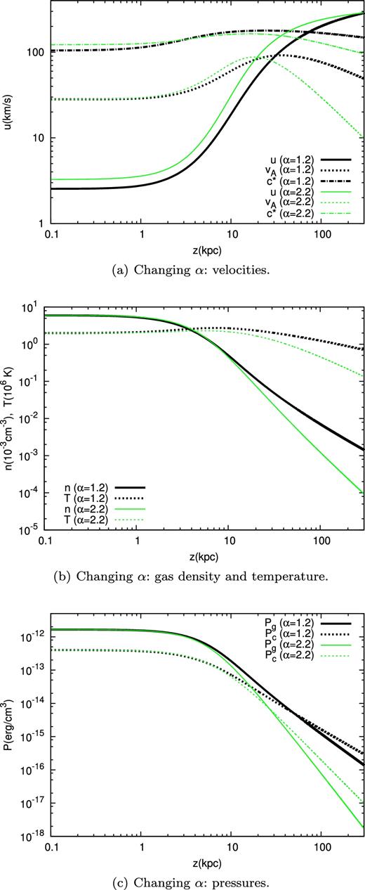
Comparison of wind profiles in case of changing the flux-tube geometry. Two cases are shown, α = 1.2 and 2.2, while the value of Zb is fixed to 15 kpc. The different plots are: (a) wind, Alfvén and compound sound speed; (b) gas density and temperature; (c) gas and CR pressures.
Dependence of the wind properties on the expansion index α. The gas density (3 × 10− 3 cm− 3), gas temperature (2 × 10⁶ K) and CR pressure (4 × 10− 13 erg cm− 3) are fixed. Zb = 15 kpc.
| α | u0 (km s−1) | zc (kpc) | uf (km s−1) |
|---|---|---|---|
| 1.2 | 2.5 | 73.0 | 513.6 |
| 1.4 | 2.7 | 61.2 | 482.0 |
| 1.6 | 2.9 | 52.6 | 453.5 |
| 1.8 | 3.0 | 45.9 | 427.6 |
| 2.0 | 3.1 | 40.6 | 403.7 |
| 2.2 | 3.3 | 36.2 | 382.0 |
| α | u0 (km s−1) | zc (kpc) | uf (km s−1) |
|---|---|---|---|
| 1.2 | 2.5 | 73.0 | 513.6 |
| 1.4 | 2.7 | 61.2 | 482.0 |
| 1.6 | 2.9 | 52.6 | 453.5 |
| 1.8 | 3.0 | 45.9 | 427.6 |
| 2.0 | 3.1 | 40.6 | 403.7 |
| 2.2 | 3.3 | 36.2 | 382.0 |
As it can be inferred from these plots, a larger value of α corresponds to smaller zc, larger u0 and smaller uf. This behaviour can be explained with considerations analogous to those invoked above for the case of a changing scaleheight Zb. At z > Zb, an increase in α corresponds to steeper density profiles (see Fig. 5b), i.e. to larger pressure gradients, which act both in the subsonic and in the supersonic region (note that in all cases zc > Zb). For this reason, when α increases, the launching velocity increases too (and consequently the mass-loss rate increases), while the terminal velocity of the wind decreases.
Note also that, as it can be seen in Fig. 5(a), the compound sound speed c* does not change appreciably when changing α, especially in the subsonic regime. Moreover, for a given Zb the area of the flux-tube A(z) does not change much for z < Zb. This leads to velocity profiles which are practically parallel up to ∼Zb at all α (see equation 24 and Fig. 5a), and to a decrease of zc when α increases. In fact, because the velocity profiles are nearly parallel within ∼Zb and c* is weakly dependent on α in the subsonic regime, at larger u0 correspond smaller zc. Finally, note the steeper c* profile at z > Zb corresponding to larger values of α. This is due to a more rapid fall off in z of the density and pressures.
5.3 Radiative cooling
For gas temperature of order ∼106 K, radiative cooling may be important and affect in a potentially important manner the properties of CR-driven winds or even the possibility to launch such winds.
Comparing the radiative cooling time and the wave heating time for the reference case of Fig. 3 (n0 = 6 × 10− 3 cm− 3), we have τcool ∼ 107 yr and τheat ∼ 108 yr. This example shows that, in the absence of additional heating terms, the radiative cooling can be a quite fast process near the Galactic (where the gas density is larger) and can in principle prevent the wind launching. From the formal point of view, a large cooling term would result in a positive numerator at the wind base in equation (32), making a wind solution impossible.
On the other hand, the ISM is also heated by SN explosions through the injection of hot gas and magnetic turbulence that will eventually dissipate into thermal energy. Recently, it was suggested that also Coulomb losses of CRs themselves might be a substantial source of heating (see Walker 2016). The relevance of cooling was already recognized by Breitschwerdt et al. (1991) which, nevertheless, assumed that some sort of energy balance must exist between heating and cooling processes. It is currently unclear which mechanism may be responsible for sufficient heating to compensate cooling, but observations reveal that the temperature in the halo is indeed in the range ∼105–106 K (see for instance Miller & Bregman 2015), hence supporting the idea that either cooling is negligible or it is balanced by one or more heating processes.
It is worth remarking that the cooling function in equation (30) has been estimated assuming that the halo has the same metallicity as the ISM in the solar vicinity, which might not be strictly true. In case of smaller metallicity, as one might expect for the gas in the halo, the cooling rate is somewhat reduced.
Given the lack of knowledge of detailed physical processes that may heat the base of the wind, here we adopted the same pragmatic attitude as Breitschwerdt et al. (1991) and assume that radiative cooling is balanced by some heating process, so as to not include an explicit heating and cooling term in the wind equations [see also (Paper I)].
However, it is worth keeping an open mind on the potentially important role of cooling in that it may induce time-dependent outflows with fall-back phenomena that cannot be treated in the context of the calculations illustrated here. Such processes require the solution of a time-dependent set of equations such as the one discussed by Dorfi & Breitschwerdt (2012). At present, a time-dependent solution that retains the kinetic form of the transport equation for CRs has not yet been implemented.
6 COSMIC RAY SPECTRUM
As discussed in the sections above, the possibility to launch a CR-driven wind and the properties of such winds depend upon the local conditions at the base of the wind, and the gravitational potential along the trajectory of the outflow. Of course, one of the important parameters of the problem is the CR pressure at the base of the wind. If we are interested in solving the problem at the position of the Sun we should recall that not only the CR pressure but also the CR spectrum is measured, so that the problem of launching a wind is much more constrained. In a non-linear theory, such as the one we adopt in this paper, the two quantities are not independent: the number of CRs at a given momentum determines the energy density of the self-produced waves and hence the diffusion coefficient, which in turn affects the spectrum and energy density of CRs. Moreover, the same quantities have a direct effect on the wind properties, which also have a feedback on the CR spectrum through advection. Note that in our iterative approach to solving the combined set of hydrodynamical equations for the wind and kinetic equations for CRs, the CR pressure is taken from observations (PCR ⊙ ∼ 4 × 10⁻¹³ erg cm−3), but the spectrum is an output of the kinetic equation. Imposing that the predicted spectrum matches the observed flux at a given energy does not ensure that the spectrum also fits observations. In fact, it is in general the case that the spectrum corresponding to wind solutions is quite unlike the CR spectrum observed at the Earth (see also the discussion in Paper I).
This will be best discussed in Section 6.1, where we present some selected cases in which we solve the wind problem for input parameters suitable for the Sun's position in the Galaxy and we check the computed spectrum versus observations. We will show that typically the CR spectrum associated to wind solutions is harder than the observed one, as a result of a dominant role of advection of CRs with the wind. In some cases, the advection velocity can be so large as to dominate the CR transport up to energies of hundreds of gigaelectronvolt. A smaller Alfvén speed (and possibly a smaller wind speed) is obtained by launching the wind with larger gas density (and/or at smaller magnetic field). On the other hand, it may happen that increasing the gas density at the base of the wind, so as to reduce the Alfvén and the wind speeds, at some point the wind can no longer be launched. In some borderline cases, whether the wind is in fact launched or not may depend on the spatial distribution of DM, namely the contribution of DM to the gravitational potential.
At CR energies (E ≳ 200 GeV), the opening of the flux-tube area together with the energy dependence of the self-generated diffusion coefficient (see equation 12) makes the CR spectrum typically steeper than the observed one. However, as discussed in Paper I, the high-energy behaviour of the CR flux may be considerably affected by the presence of non-self-generated turbulence in the near disc region (within ∼1 kpc from the base of the wind). In fact such turbulence should be postulated in this class of models if to account for the spectral hardening measured by the PAMELA Adriani et al. (2011) and AMS-02 Aguilar et al. (2015) experiments.
In Section 6.2, we discuss the impact of the DM halo profile on the CR spectrum, and we show that it is possible to find a wind model which is consistent with both the recent observations illustrated by Miller & Bregman (2015) and with the observed CR spectrum.
6.1 Reference models
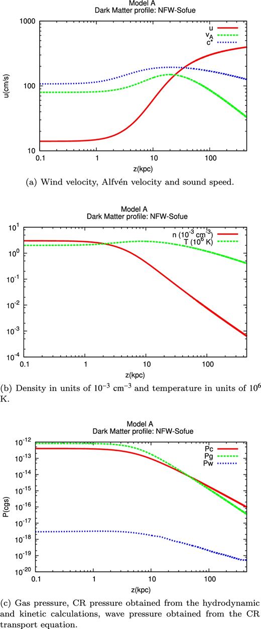
Results for Model A: at the wind base, z0, the gas density is n0 = 3 × 10− 3 cm− 3 and the magnetic field is B0 = 2 μG. The CR injection spectrum has been normalized in order to get the observed CR pressure Pc0 = 4 × 10− 13 erg cm− 3 at z0.
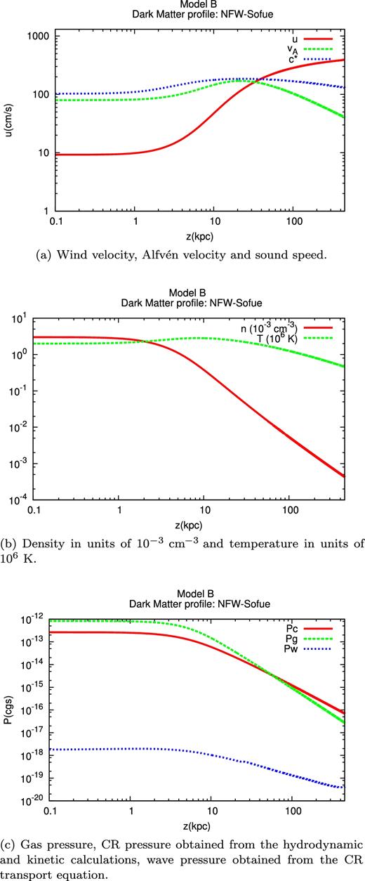
Results for Model B: at the wind base, z0, the gas density is n0 = 3 × 10− 3 cm− 3 and the magnetic field is B0 = 2 μG. The CR injection spectrum has been normalized in order to reproduce the observed CR spectrum at 50 GeV.
The wind velocity, the Alfvén speed and the compound sound speed for Model C are shown in Fig. 8(a), while Fig. 8(b) illustrates the evolution of the wind density and temperature. The wind is launched sub-Alfvénic with u0 = 2 km s−1 and becomes sonic at zc = 60 kpc, while the Alfvén speed at z0 is 28 km s−1. The CR pressure is shown in Fig. 8(c), together with the gas and the wave pressure. As for Model B, the CR pressure at z0 is an output of the calculation, Pc0 = 3.2 × 10− 13 erg cm− 3.
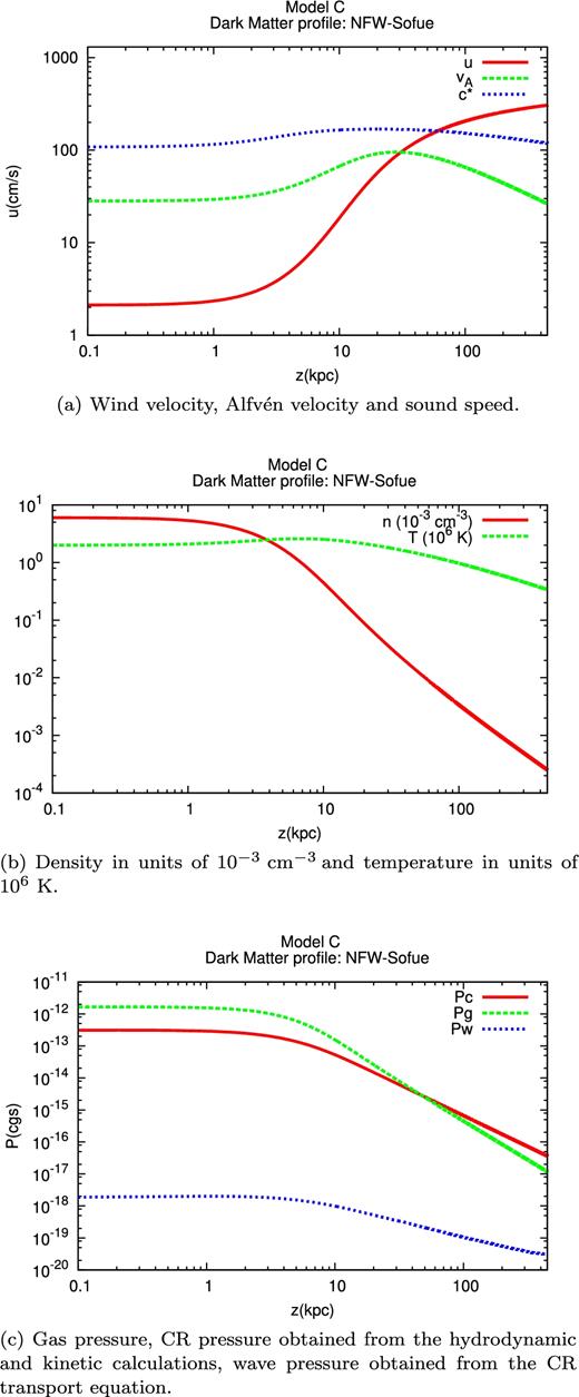
Results for Model C: at the wind base, z0, the gas density is n0 = 6 × 10− 3 cm− 3 and the magnetic field is B0 = 1μG. The CR injection spectrum has been normalized in order to reproduce the observed CR spectrum at 50 GeV.
The spectrum of CR protons at the position of the Sun in the three scenarios discussed above is shown in Figs 9(a)–(c) compared with the proton flux as measured by the voyager-i Stone et al. (2013) at low energies and by AMS-02 Aguilar et al. (2015) at higher energies. The red curve illustrates the effect of solar modulation, with the simple recipe of Bernardo et al. (2010). One should not overestimate the importance of the comparison of our predicted CR spectrum with observations at energies below ∼1 GeV, because in such energy region, energy losses become important and such effects have not been included in the calculations presented in this paper.
In all the three cases introduced above, the CR advection velocity near the wind base is dominated by the Alfvén speed. The advection velocity at the wind base is u0 + vA0 ∼ 93, ∼88 and ∼30 km s−1 for Models A, B and C, respectively. An important feature of the spectra in the disc, shown for the three models in Fig. 9, is the presence of hard spectra which extend to higher energies for increasing advection velocity. This is due to the fact that, the larger the CR advection velocity, the higher the CR energy at which advection dominates upon diffusion in the CR transport equation, thus producing a spectrum with spectral index close to the injection spectral index.
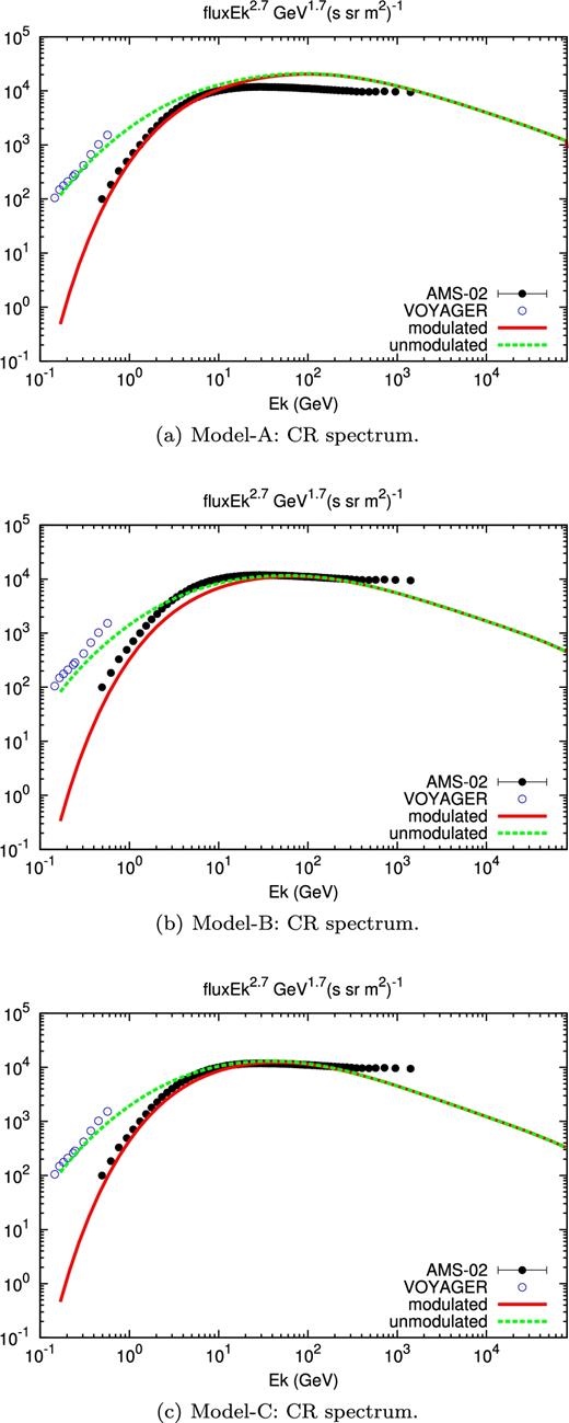
CR spectrum compared to the voyager and AMS-02 data for Models A, B and C. Solar modulation has been applied with Φ = 500 MV.
From Fig. 9(c), one can see that below ∼200 GeV Model C resemble the observed CR spectrum, while the harder spectra in Models A and B appear to be quite unlike the observed one, even qualitatively. This is a rather general conclusion: even using values for the environmental parameters that are compatible with observations (see Section 5) and that lead to wind launching, the corresponding CR spectrum at the Sun's position is, in general, qualitatively different from the observed one, even if the total CR pressure may be close to the measured one.
Making use of the points discussed in Section 5 concerning the dependence of the wind properties on the launching parameters, we can infer what would happen by changing the gas density and temperature and the magnetic field at the wind base (always within the observational constraints). By increasing the magnetic field and/or decreasing the gas density, the Alfvén speed would increase and, consequently, harder spectra would be inferred. In addition, a decrease of the gas density, as well as an increase of the gas temperature, leads to an increase of the wind launching velocity, with similar implications for the CR spectrum. On the other hand, an increase in the gas density would lead to smaller advection velocities (decreasing both the Alfvén and the wind speeds), hence a generally steeper spectrum. However, when the density becomes too high it may become impossible to launch a wind. The same considerations hold when decreasing the gas temperature: the Alfvén speed is not affected but the wind velocity decreases. This situation is particularly important for winds in which the launching velocity is comparable or larger than the Alfvén speed. Also in this case, for smaller temperatures the wind launching may be inhibited.
6.2 Models versus observations: the effect of the dark matter halo
Here, we present a wind model whose parameters are compatible with properties of the Galactic halo derived in Miller & Bregman (2015), i.e. Model C of Section 6.1 (see discussion below), and we study how the CR spectrum depends on the DM halo profile. In particular, we show that it is possible to have a good agreement with the observed CR proton spectrum, depending on the choice of the DM halo potential.
In Fig. 11(a), we show the wind density and temperature obtained with the input parameters of Model C and for the three DM haloes NFW–Sofue, BUR and EIN. The NFW–Salucci model is missing since with such halo no wind was launched. This is a typical example of how, fixed any other parameter, an increase of the gravitational pull (the NFW–Salucci has the largest force among the proposed models) could prevent the wind launching. In Figs 10(a) and (b), we show the corresponding wind speed, sound speed and Alfvén velocity, while in Fig. 11(b), we show the gas and CR pressures. For all the three DM models, the wind is launched as sub-Alfvénic with: (u0 = 2 kms− 1, zc = 60 kpc, uf = 450 kms− 1) for the NFW–Sofue profile, (u0 = 3 kms−1, zc = 285 kpc, uf = 273 kms−1) for the BUR profile and (u0 = 2.7 kms−1, zc = 590 kpc, uf = 253 kms−1) for the EIN profile.
The mass-loss rate and the halo mass of the wind is |$(\dot{M} = 0.46\, {\rm M_{{\odot }} yr^{-1}},\, M(<50\, {\rm kpc}) \sim 1.2\times 10^9\,\ {\rm M_{{\odot }}}, \, M(<250\, \rm kpc) \sim 1.9\times 10^9 \rm \,M_{{\odot }})$| for the NFW–Sofue profile, |$(\dot{M} = 0.7\, {\rm M_{{\odot }} yr^{-1}},\, M(<50\, {\rm kpc}) \sim 3.2\times 10^9\ {\rm M_{{\odot }}}, \, M(<250\, \rm kpc)\sim 6.4\times 10^9\, \rm M_{{\odot }})$| for the BUR profile and |$(\dot{M} = 0.63\, {\rm M_{{\odot }} yr^{-1}},\, M(<50\, {\rm kpc}) \sim 3.1\times 10^9\, {\rm M_{{\odot }}}, \, M(<250\, \rm kpc) \sim 8\times 10^9\, \rm M_{{\odot }})$| for the EIN profile. Such values of the halo mass are of the same order of magnitude of the Galactic halo mass estimated by Miller & Bregman (2015, M( < 50 kpc) ∼ 3.8 × 10⁹ M⊙, M( < 250 kpc) ∼ 4.3 × 10¹⁰ M⊙).
Note that at larger gravitational acceleration, i.e. for the NFW–Sofue profile, we get a smaller launching velocity u0 and a larger terminal velocity uf. Moreover, we get a smaller zc. This fact can be explained as follows: in the subsonic regime, the gravitational term dominates the numerator of the wind equation (3), while c* is weakly dependent on the DM profile (see Fig. 10). Thus, a larger gravitational force leads to a larger gas acceleration in the subsonic region, large enough to provide a smaller zc despite the smaller launching velocity, as it can be seen in Fig. 10. The rapid increase of the wind velocity, which starts at smaller z and with a steeper profile for the NFW–Sofue, corresponds to the rapid decrease of the gas density and of the CR and gas pressure (see Figs 11a and b). In the range z ∼ 1–100 kpc, the NFW–Sofue profile shows the largest Alfvén speed (due to the smaller gas density), and the smallest CR pressure. However, the first effect is still dominant, leading to a larger heating due to wave damping (recall that the heating term is ∼vA∇Pc), and hence to a slightly larger temperature (see Fig. 11a) compared to the BUR and EIN haloes. Note that the effect of wave damping is in fact to keep the gas temperature around 2 × 10⁶ K up to ∼100 kpc (this is especially true for the NFW–Sofue profile), in line with the results of Miller & Bregman (2015) on the Galactic halo temperature.
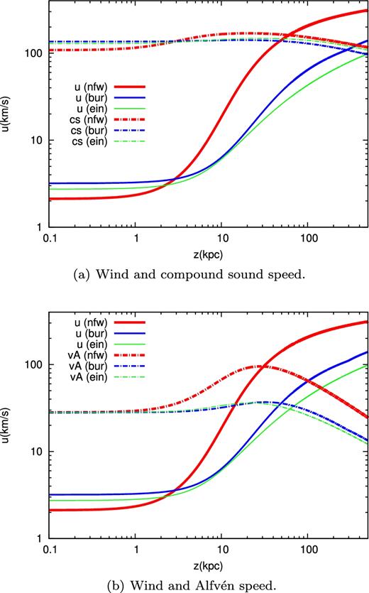
Dependence of the CR spectrum on the DM halo: (a) wind and compound sound speed; and (b) wind and Alfvén speeds.
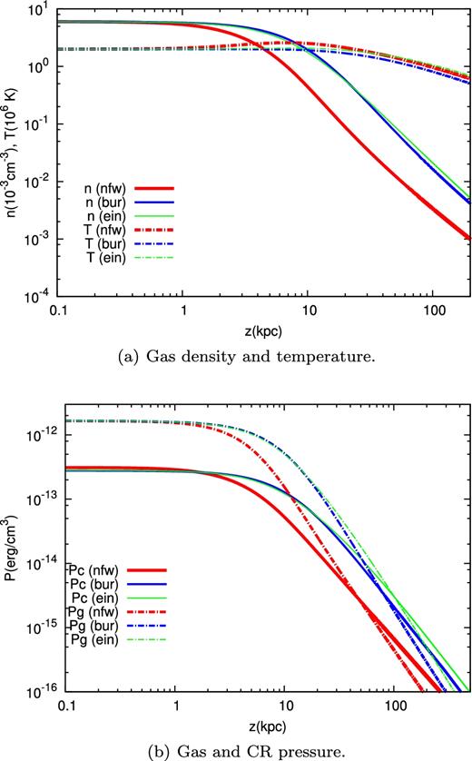
Dependence of the CR spectrum on the DM halo: (a) gas density and temperature; and (b) gas and CR pressures.
In Fig. 12, we show the CR spectrum for the NFW–Sofue, BUR and EIN profiles. Below ∼200 GeV, the best (qualitative) match to the observed proton spectrum is achieved with the NFW–Sofue model. The larger wind launching velocity of the BUR and EIN models leads to a low-energy spectrum harder than the observed one.
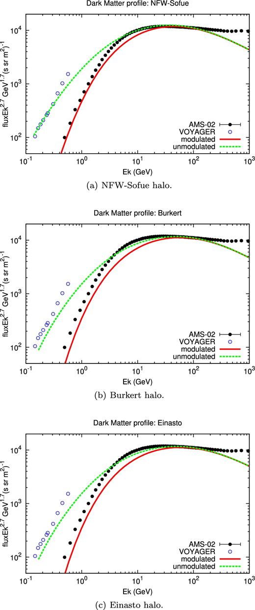
Dependence of the CR spectrum on the DM halo: (a) CR spectrum with the NFW halo; (b) CR spectrum with the BUR halo; (c) CR spectrum with the EIN halo.
7 CONCLUSIONS
In this paper, we studied the possible presence of CR-driven Galactic winds launched at the Sun location and the dependence of their properties and of the related CR spectrum on the conditions of the Galactic environment in the vicinity of the Sun. We used the semi-analytical calculation developed in Paper I, which allows to compute at the same time both the hydrodynamical structure of the wind, the CR distribution function and CR self-generated diffusion coefficient. The CR transport is considered to be due to the diffusion off Alfvén waves generated by CRs through streaming instability, saturated through NLLD, and to the advection with such waves and with the wind. The wind launching and the CR spectrum depend on the properties of the ISM (gas density and temperature, Galactic magnetic field), on the CR injection, on the flow geometry and on the Galactic gravitational potential. All these quantities depend on the position in the Galaxy and are constrained by observations.
We found that, in agreement with previous hydrodynamic calculations of CR-driven winds, the combined action of the thermal and CR pressures can drive winds for a variety of environmental conditions. In particular, it is possible to launch winds with input parameters compatible with observations of the ISM in the vicinity of the Sun. We also found that in many cases, winds launched with environmental parameters compatible with observations lead to a CR spectrum which is not in agreement with the observed one. As pointed out in Paper I, this is mainly due to the fact that CR advection in such winds is strong, leading to spectra at low energies (below ∼200 GeV) which are harder than the observed spectrum. At high energy (above ∼200 GeV), instead, the wind expansion, together with the steep energy dependence of the self-generated diffusion coefficient, leads to spectra which are steeper than the observed spectrum. However, the high-energy spectrum may be affected by other factors, such as the presence of turbulence non-generated by CRs (Aloisio et al. 2015, Paper I).
As for the low-energy part of the spectrum, we found that it is possible to find specific cases in which the wind launching parameters and the resulting wind properties are compatible with observations, in particular with the Galactic halo properties deduced by Miller & Bregman (2015), and the resulting CR spectrum is also in agreement with observations. In this analysis, we also found that an important role is played by the choice of the DM halo model. In fact, we showed that, for given values of all parameter, the DM gravitational potential can determine whether the wind is launched and the quality of the agreement with the observed CR spectrum.
This analysis highlights that the low-energy part of the CR spectrum provides a strong constraint for wind models and that an accurate modelling of the Galactic environment and of the Galactic gravitational potential (in particular of the DM halo) are of crucial importance in the understanding of Galactic winds.
The study presented here can be extended to any other locations in the Galaxy different from the Sun's position and can be used to analyse the possible presence of winds and the related CR spectrum in the whole Galaxy. Such investigation would allow us to calculate the rate of mass loss and the mass of the baryonic halo induced by the wind (both are crucial ingredients in models of galaxy formation and evolution), as well as the expected intensity in emission and absorption lines from the halo (for instance in the X-ray band) and the CR density gradient in the Galaxy (which can be tracked by the γ-ray emission resulting from CR interactions with the background plasma).
There is much room for improvement of the model presented here and such developments appear necessary if to address some physical problems, such as time-dependent effects induced by cooling in the halo and the interplay between the outflows associated with the CR-induced wind and the presence of a possible accretion of material from the IGM.
Acknowledgments
The authors are glad to acknowledge a continuous ongoing collaboration with the rest of the Arcetri high energy Group. Giovanni Morlino wants also to acknowledge the hospitality of International Space Science Institute for Teamwork 351 on ‘The origin and composition of Galactic cosmic rays'.
REFERENCES
