Voids and superstructures: correlations and induced large-scale velocity flows Free

Abstract

1 MOTIVATION

The cosmic web is the largest scale outcome of the anisotropic growth of mass overdensities. It also represents the transition between the linear and non-linear regimes and encodes information about the early phases of structure formation. The analysis of the mass transport between different environments clearly shows how matter flows from voids into walls, and then via filaments into cluster regions, which form the nodes of the cosmic web (see e.g. Van de Weygaert & Platen 2011; Cautun et al. 2014), producing different redshift evolution of haloes in different environments (Hahn et al. 2007).

The relations between the different types of the largest structures in the universe have been suggested on several contexts (Einasto, Saar & Klypin 1986; Einasto et al. 1997; Platen, van de Weygaert & Jones 2008; Aragón-Calvo et al. 2010; Einasto et al. 2011). This allows to analyse the large-scale structure in terms of the large overdense structures or alternatively in terms of the large underdense regions. Actually, the largest overdense structures that shape the cosmic web also serve as boundaries for voids (Cautun et al. 2014). Also, by understanding the evolutionary processes of the different structures we can obtain a deeper insight into the origin and history of the present structure (Leclercq, Jasche & Wandelt 2015).

In order to deepen our understanding on the nature of voids and the evolution of their properties, it is crucial to take into account the surrounding environment where they are embedded (Paranjape, Lam & Sheth 2012). Essentially, the hierarchy of voids arises by the assembly of mass in the growing nearby structures. Sheth & van de Weygaert (2004) suggest that while some voids remain as underdense regions, other voids fall on to themselves due to the collapse of dense structures surrounding them. According to this scenario, void evolution exhibits two opposite processes, expansion and collapse, being the dominant process determined by the global density around the voids. The distinction between these two types of void behaviour depends on the surrounding environment. It is expected that the large underdense regions with surrounding overdense shells will undergo a void-in-cloud evolution mode. These voids are likely to be squeezed as the surrounding structures tend to collapse on to them. On the other hand, voids in an environment more similar to the global background density will expand and remain as underdense regions following a so-called void-in-void mode. In a series of works (Ceccarelli et al. 2013; Paz et al. 2013; Ruiz et al. 2015), we have considered an alternative classification of void according to their environment taking into account the cumulative radial density profiles. Voids with a surrounding overdense shell exhibit a rising cumulative density profile, which overcompensates the underdensity and therefore reach positive values between two and three times the void radius. These voids, dubbed S-type after its shell-like structure, are likely collapsing. On the other hand, voids with a smoothly rising integrated density profile that approaches the mean density at large distances (hereafter R-type voids) show a continuous expansion. In this scheme, R-type voids resemble void-in-void objects while void-in-clouds are consistent with the S-type definition.

The origin of the large-scale flows observed in the local Universe has been the subject of controversy during the last decades. While several works have focused on the search of a great attractor consistent with peculiar velocities of local structures, an alternative approach includes the expansion of the local void as proposed by Tully et al. (2008, 2014). Albeit the contribution of the local void dynamics improves the description of the velocity fields in the nearby Universe, the estimated peculiar velocity of the Local Group is still conflicting with that predicted from the infall on to the Shapley supercluster and the local void expansion due to the presence of residual velocities of ∼200 km s⁻¹ for the Local Group (van de Weygaert 2016, and references therein).

In recent works, we have reported the non-negligible motions of voids as a whole (Ceccarelli et al. 2016; Lambas et al. 2016), adding a new component affecting galaxy peculiar velocities. These global motions can be a key piece to complete the scenario of the dynamics of local structures. In this work, we show that the velocities generated by the mass under/overdensities associated with the large-scale structures of the galaxy distribution are complementary to obtain a detailed description of the large-scale velocity flows. In this context, we study the joint dynamics of galaxies with respect to voids and future virialized structures (hereafter FVSs), in order to explore coherent patterns of motions of mass from the shells of voids to the largest overdensities.

In the next section, we describe the general methods used to identify voids and FVSs, both in semi-analytic galaxies and in an observational galaxy catalogue. Then, in Section 3 we analyse the spatial distribution of voids relative to superstructures and their associated dynamics. The same analysis is then performed to galaxies, where their motions are considered separately for different configurations of relative positions of galaxies, voids and FVSs. In Section 4, we also present similar studies applied to observational data. Finally, we present a discussion of our results in the context of recent works in Section 5.

2 DATA

2.1 Galaxy catalogues

The observational galaxies used in this work correspond to the Main Galaxy Sample of the Sloan Digital Sky Survey Data Release 7 (SDSS-DR7, Abazajian et al. 2009). This catalogue comprises almost a million of spectroscopic galaxies with redshift measurements up to z ≤ 0.3 and an upper apparent magnitude limit of 17.77 in the r-band. From this sample, we select galaxies with a limiting redshift z = 0.12 and a maximum absolute magnitude in the r-band of M_r − 5 log₁₀(h) = −19.95, in order to obtain a volume complete sample of galaxies at that redshift. The limits of this sample are chosen on the basis of a compromise between the volume and the number of tracers. For SDSS velocities, we adopt the peculiar velocity field presented by Wang et al. (2012). The authors used the linear theory connection between mass overdensity and peculiar velocity to reconstruct the 3D peculiar velocity field of SDSS galaxies (Wang et al. 2009). With this velocity field we compute the bulk void velocities in the SDSS sample. For an analysis of the effects of using linearized velocities, we refer the reader to the appendix of Ceccarelli et al. (2016). We also analysed the influence of large-scale flows in observational data. For this purpose, we used a galaxy group catalogue which follows the identification method presented in Yang et al. (2005), applied to SDSS-DR4 in Yang et al. (2007) and updated by the authors to the SDSS-DR7.¹ For this sample of groups, we also adopted the linearized velocity field by Wang et al. (2012).

On the other hand, the simulated galaxies used were extracted from a semi-analytical model (SAM) of galaxy formation applied to the Millennium Simulation (MS; Springel et al. 2005), a cosmological N-body simulation that counts with 2140³ dark matter particles evolved in a cubic comoving box of 500 h⁻¹ Mpc on a side. The cosmological parameters adopted for the MS correspond to WMAP1 results (Spergel et al. 2003), i.e. a flat Λ cold dark matter cosmology with Ω_m = 0.25, |$\Omega _\Lambda = 0.75$|⁠, Ω_b = 0.045, σ₈ = 0.9, h = 0.73 and n = 1.0. Given that the MS is a dark matter-only simulation, their dark matter haloes need to be populated with a SAM to obtain a galaxy population. In this work, we use the public catalogue developed by Guo et al. (2011), which is available at the Millennium Database.² In order to make a fair comparison between observations and simulated data for the complete simulated galaxy population, we select a sample with the same number density than the observations This was achieved by selecting all galaxies brighter than M_r − 5 log h = −20.6, which guarantees the volume density required. Although this threshold in absolute magnitude is not the same as the limiting magnitude used to define the volume-limited sample of galaxies, it satisfactorily reproduces the distribution of galaxies (see e.g. Contreras et al. 2013, 2015). The difference between the two values arises from the fact that semi-analytical models do not exactly reproduce the luminosity function of galaxies in SDSS.

2.2 Catalogues of cosmic voids

To construct the void catalogue, we follow the procedure described in Ruiz et al. (2015), which is a modified version of the algorithms presented in Padilla, Ceccarelli & Lambas (2005) and Ceccarelli et al. (2006). The galaxies (either simulated or observed) are the tracers of the density field used in void for the identification. The method starts with a contrast density field estimation performed with a Voronoi tessellation, where underdense cells are selected as void candidates. Centred in those positions, we compute the integrated density contrast Δ(r) at increasing values of radius r, selecting as void candidate the largest spheres that satisfy the condition Δ(R_void) < −0.9 and defining R_void as the void radius. Afterwards, the centre position of void candidates are randomly tilted and the sphere is allowed to grow in order to recentre the void. Finally, a void of radius R_void is selected as the largest sphere satisfying the underdense condition and not overlapping with any other underdense sphere. The final catalogues comprises 1676 voids for the full Millennium box and 495 voids for the total SDSS sample, but for dynamical analyses we used only 288 of them (121 R-type and 167 S-type), which belong to the inner region of the survey where the velocity field of Wang et al. (2012) has a reliable reconstruction. The void radii are in the range 8–26 h⁻¹ Mpc, both in SDSS and the simulation.

2.3 Catalogues of superstructures

In previous works, we have defined the procedures to select superstructures that will be virialized systems in the distant future (Luparello et al. 2011). The criteria applied can be used for both observational and simulated galaxy catalogues. The method relies on the computation of the luminosity density field, by convolving the spatial distribution of galaxies (either observed or SAM) with a kernel function weighted by galaxy luminosity. We adopted an Epanechnikov kernel of 8 h⁻¹ Mpc to sample the density field into a grid composed by cubes of 1 h⁻¹ Mpc side. We then select the highest luminosity density groups of cells to isolate the large structures that will become virialized systems in the future (Dünner et al. 2006). In our final catalogue we identified 150 FVSs comprising 11 394 galaxies in the SDSS, out of which 105 FVSs are within the region where we used the reconstructed velocity field data by Wang et al. (2012). The simulation, on the other hand, has 790 FVSs due to its larger volume, which is approximately six times the SDSS volume.

3 ANALYSIS IN THE SIMULATION DATA

Here, we present the main results obtained from the analysis of voids and FVSs identified in the simulated galaxy catalogue. In what follows, we develop a measurement for the correlation between extended regions corresponding to voids and FVSs and analyse their associated dynamics.

3.1 Spatial distribution of voids relative to FVSs

The definition of voids and FVSs results in two types of structures that are distributed in space occupying somewhat complementary locations. In this context, it is worth asking if these structures are related in a non-trivial fashion (i.e. if their distributions are consistent with a random distribution or if the locations of overdense structures affect the locations of underdense structures). In Lares et al. (2017), we show that the spatial locations of voids are correlated with voids with the same environment (void-in-void or void-in-cloud types) giving rise to void clumps. According to this study, clumps of R-type voids show a dynamical behaviour consistent with divergent flows, produced by a combination of mutually receding and expanding voids. On the other hand, clumps of S-type voids exhibit large-scale flows that are predominantly infalling towards the clump centre. The global density of these clumps is, in most cases, positive. This implies that there must be overdense structures inside clumps which compensate the void underdensities. In reference to these ideas, we show in Fig. 1 a visualization of an FVS and its nearby voids for a subset in the simulation. We included a visualization of a group of void–FVS pairs, including all the voids (represented as spheres) that have the FVS (in the centre of the figure) as their closest one. Arrows are scaled representations of the void velocity vector, with dotted segments located inside or behind voids. Other FVSs and voids in the neighbourhood are not shown for simplicity. In this context, we argue that large-scale flows play a key role in the formation of the supercluster–void network, and that superclusters might be responsible for the global collapse.

Figure 1.

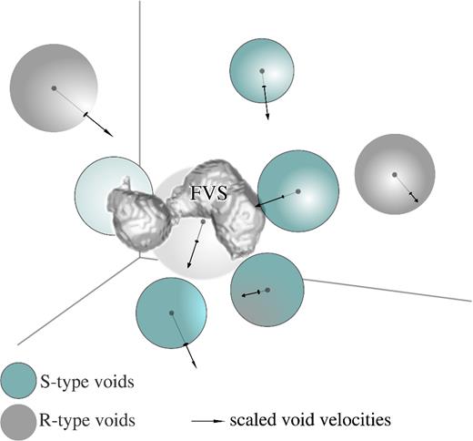
A visualization of a group of void–FVS pairs, including all the voids (represented as spheres) that have the FVS (in the centre of the figure) as their closest one. Arrows are scaled representations of the void velocity vector, with dotted segments located inside or behind voids. This example corresponds to a subset of data from the simulation. Other FVSs and voids in the neighbourhood are not shown for simplicity. Darker spheres represent R-type voids and delineated spheres represent S-type voids. The latest are typically closer and moving towards the FVS.

Open in new tabDownload slide

Here, we focus on the relation between the positions and dynamics of voids relative to FVSs. The most common used statistic to quantify the relative distributions of two types of points is the two-point cross-correlation function, defined as the excess probability of finding a pair of objects at a given separation compared to that expected from a random distribution. However, neither voids nor FVSs can easily be represented by a point location. Voids are characterized by a centre and a radius or scale. Moreover, FVSs do not have a simple shape and a centre cannot be clearly defined.

We define a procedure to quantify the relative clustering of voids and FVSs as follows: if the locations of voids and FVSs are both random and independent, the probability for a randomly placed sphere to be in contact with both types of structures should equal the product of the probability that the sphere touches a void times the probability of touching an FVS. These measures certainly depend on the size of the sphere, but if the distributions of the two types of structures are completely uncorrelated, the two probabilities are expected to be roughly the same. If, on the other hand, they are different, it would indicate a systematic tendency of either correlation (positive excess) or anticorrelation (negative excess) with respect to FVSs.

Figure 2.

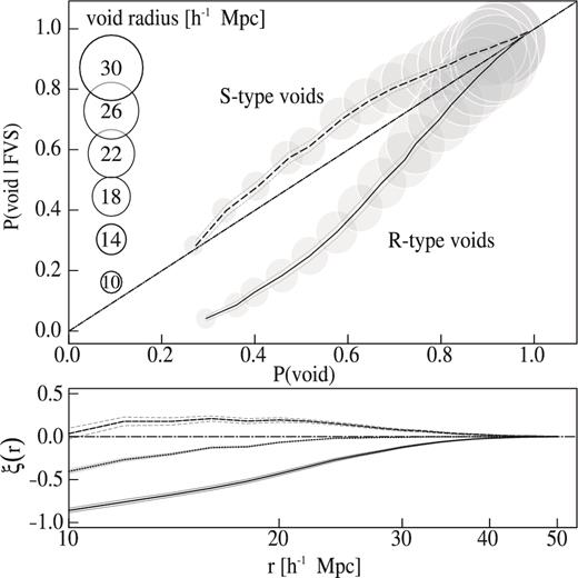
Spatial distribution of voids with respect to FVSs, in the simulation. Upper panel: the curves show the conditional probability, P(void|FVS), of finding a randomly placed sphere containing simultaneously void and FVS volume fractions, as a function of the probability P(void) that the sphere contains a fraction of void volume, in spite of the presence of FVS. If the locations of voids and FVSs were independent, P(void|FVS) ≃ P(void) for any value of sphere radius (dot-dashed line indicating a one-to-one relation). The upper curve corresponds to the results for S-type voids and the lower curve to R-type voids. Circle radii scale linearly with the radius of the random spheres. Uncertainties are computed using Jackknife resamplings. Bottom panel: void–FVS correlation function ξ(r). We use the definition of ξ(r) − ξ_void-FVS(r) given in equation (4). S-type voids exhibit a positive correlation in a wide range of scales, consistent with their denser environment. On the other hand, R-type voids and FVSs are anticorrelated, with a stronger signal than that of S-type voids. The central curve corresponds to the full sample of voids, without separating by type.

Open in new tabDownload slide

In the bottom panel of this figure, we show the void–FVS correlation function ξ_void-FVS(r) for S-type voids (upper curve, dashed line), R-type voids (bottom curve, solid line) and the combined sample of voids including both types (dotted line). It follows the definition of the correlation function given in equation (4). It is worth noticing that FVSs represent a small fraction of the total simulation box volume (nearly 4 per cent; see Luparello et al. 2011) while voids comprise almost 20 per cent of the volume.

3.2 Dynamics of voids relative to FVSs

In the previous section, we showed that there is a tight relation between the locations of voids of different types and the locations of FVSs. Moreover, this geometrical property in the distribution of the largest scale structures should also have a dynamical counterpart. The arguments presented in Section 1 suggest that the large-scale flows are closely related to the evolution of the largest scale structures, and consequently a dynamical connection between voids and FVSs is expected. Although the choice of the spherical approximation of voids is suitable, FVSs cannot be described with simple geometrical objects, which implies that quantities such as relative distance, position or velocity between those two types of structures are not straightforward to compute.

Here, we adopt a simple approach that takes into account basic dynamical principles and allows to study the joint dynamical behaviour of voids and FVSs. To analyse the dynamic of FVS–void pairs, as the first step we identify the nearest FVS for each void. Since the FVSs have complex shapes, we consider the core region of each FVS, defined as the volume covered by the highest density cells. As we mentioned in Section 2.3, in the identification of these structures we have used a physically motivated threshold on luminosity overdensity (Luparello et al. 2011), following the criteria calibrated on simulations by Dünner et al. (2006). According to this procedure, we chose a ratio of luminosity density, ρ_lum, relative to the mean satisfying |$\rho _{\rm lum} / \overline{\rho }_{\rm lum}>5.5$| to define the boundaries of an FVS in a 3D grid-averaged smoothed density field estimation. Thus, since the densest region of the FVSs roughly matches the central region, we define as the central, denser component of an FVS all cells having |$\rho _{\rm lum} / \overline{\rho }_{\rm lum}>6.3$| (corresponding to the median of the luminosity density distribution of FVS cells). The distance between a void and an FVS is then defined as the distance between the void centre and the closest cell of the densest core of the FVS. For each of the closest void–FVS pair, we compute their relative position and velocity. To this aim, we define the velocity of the closest FVS cell as the average of the velocities of the galaxies inside a sphere centred in the high density cell and with radius equal to the distance between the void centre and this cell. The void velocity is then taken relative to their corresponding closest high density cell. The angle between these relative position and velocity vectors, θ, allows to study the flow on to FVSs.

Figure 3.

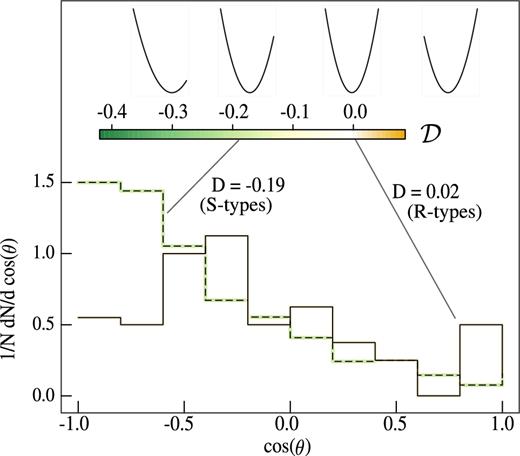
Normalized histograms of the distribution of cos(θ), where θ is the angle between the relative velocity and the relative position of the void–FVS system (see the text for details), for subsamples of R-type voids (dotted line) and for S-type voids (solid line) in the simulation. These subsamples were chosen in order to show the different values of |$\mathcal {D}$|⁠. One sample comprises R-type voids with a separation from the FVS greater than d > 40 h⁻¹ Mpc and M<10¹⁴h⁻¹ M_⊙. The sample of S-type voids is restricted to d < 40 h⁻¹ Mpc and M >10^14.2 h⁻¹ M_⊙. On the top of the figure, we show a scale indicating the values of the dipole coefficient |$\mathcal {D}$| for both samples. We also show, for reference, model distributions for different values of the dipole coefficient (−0.4, −0.2, 0 and 0.2, respectively).

Open in new tabDownload slide

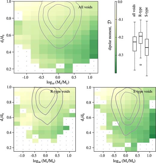
In the upper panel of Fig. 4, we show the dipole moment |$\mathcal {D}$| of the cos (θ) distributions in bins of FVS mass M₁ and void–FVS distance d₁. As shown in this figure, the higher negative values of the dipole (that indicates an infall signal for the pairs) mainly occurs when the voids are located close to an FVS. This statistical excess is significant even at distances as large as 50 h⁻¹ Mpc. However, it is important to note that besides the low number of objects, the higher values of |$\mathcal {D}$| correspond to the most massive FVSs. In grey, we show the level curves of the number of pairs of FVS–void which correspond to the 25, 50 and 75 per cent of the sample. White bins, with a central dot, do not contain any pair. For the rest of the matrix, we applied a smoothing kernel using a top-hat window of two bins each side (ignoring empty bins). The colour scale indicates the values of the |$\mathcal {D}$| statistic defined in equation (5). The limits of this scale are the same as the colour scale in Fig. 3, which gives a picture of the degree of anisotropy that corresponds to the different values of the |$\mathcal {D}$| statistic. In the left- and right-hand lower panels of Fig. 4 we show the dipole moment for R-type and S-type voids, respectively. Box plots correspond to the distributions of |$\mathcal {D}$| for each sample. There is a stronger infall signal for S-type voids, which is noticeable up to nearly 25 h⁻¹ Mpc of void–FVS separation. Also, in agreement with the results of the previous section, it can be noticed that S-type voids tend to be located closer to superstructures than R-type voids.

Figure 4.

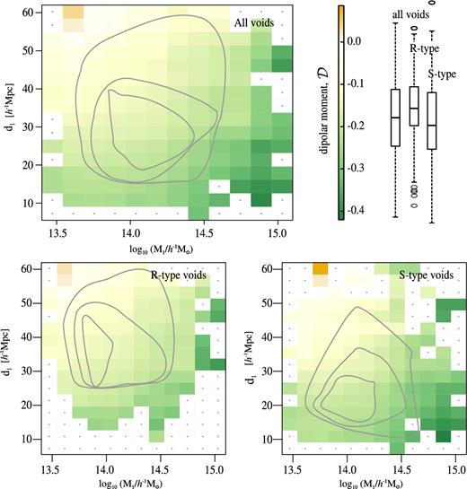
Dependence of the dipole moment on FVS mass and void–FVS separation in the simulation data. We show 2D histograms of the dipole moment estimator |$\mathcal {D}$| (encoded in colour) for the distribution of cos(θ) in bins of FVS mass and void–FVS distance. Positive values of cos(θ) correspond to the positive velocity components on the FVS-void direction (see the text for its definition), which indicates that the void is moving away their closest FVS. We show in the upper panel the full sample of void–FVS pairs and in the bottom left-hand and right-hand panels the R- and S-type voids, respectively. Box plots correspond to the distributions of |$\mathcal {D}$| for each sample. Contour levels are shown for the number of objects contributing to the signal in each bin and correspond to 25, 50 and 75 per cent of the pairs.

Open in new tabDownload slide

However, these results are obtained taking into account only the nearest FVS to each void. The possible presence of other structures at similar distances leads us to take into account the influence of at least the second nearest structure. To this aim, we compute the relative distance between the void and their nearest FVS (d₁) and the void and their second nearest FVS (d₂), and the ratio of the corresponding FVSs distances and masses. Following the same scheme of Fig. 4, in Fig. 5 we show the dipole moment as a function of the relative distances and masses. The data shown in these figures are not exactly the same due to different mass and distance limits, which produce slightly different box plots. Here, we can see that if the nearest FVS is remarkably closer to the void there is a clear infall signal and this intensifies if the nearest FVS is much more massive than the second one. In this figure, we distinguish R- and S-types showing S-type voids preferentially located closer to their nearest superstructure. In Fig. 6, we show the cumulative distributions of void–FVS distances (bottom and right scales) for R/S-types and for different void radius intervals (10.0 < R_v/(Mpc h^{− 1}) < 12.5 with dotted lines, 12.5 < R_v/(Mpc h⁻¹) < 15.0 with thin solid lines and 15.0 < R_v/(Mpc h⁻¹) < 17.5 with thick solid lines. The histograms show the distributions of void radii for the two void types (upper scale, with arbitrary normalization), with filled bars for S-types and empty bars for R-types. The shifts in the cumulative distributions are larger considering void type, indicating that it is not dominated by void-size segregation. Also, in S-type voids we can see that the infall signal grows when the mass of their nearest FVS (M₁) is greater than the mass of the second one (M₂).

Figure 5.

2D histograms of the dipole moment estimator |$\mathcal {D}$| for the distribution of cos(θ), in bins of the ratios of masses and distances between the closest and the second closest FVS to each void. This estimator is computed for the closest void–FVS pair. Box plots and contour levels are analogous to those of Fig. 4.

Open in new tabDownload slide

Figure 6.

Cumulative distributions of void–FVS distances (bottom and right scales) for R/S-types and for different void radius intervals (10.0 < R_v[h⁻¹ Mpc] < 12.5 with dotted lines, 12.5 < R_v[h⁻¹ Mpc] < 15.0 with thin solid lines and 15.0 < R_v[h⁻¹ Mpc] < 17.5 with thick solid lines). The histograms show the normalized distributions of void radii for R-types (empty bars) and S-types (filled bars). It can be clearly seen that the difference in the FVS-void distance cumulative distributions is dominated by void type and not by void size.

Open in new tabDownload slide

3.3 Galaxies in void shells

In order to study the influence of the large-scale flows on galaxies, we analyse the velocity field related to the spatial configuration of the systems. To this aim, we use SAM central galaxies and identify their nearest FVS to calculate their relative projected velocity. Our sample comprises 79 403 galaxies, out of which 1996 are located in R-void shells and 3364 in S-void shells. We also distinguish between galaxies located in void shells or elsewhere and we restrict to galaxy–FVS distances in the range 10–40 h⁻¹ Mpc. In the upper panel of Fig. 7, we show the mean projected velocity, V cos(θ), of galaxies in void shells as a function of their relative angle, ϕ, with respect to the direction that connects the void centre and the nearest FVS, as outlined in the scheme. The location of a galaxy in the void shell with respect to the FVS direction is given by cos (ϕ). Galaxies in the cap facing the FVS have cos (ϕ) > 0 and galaxies opposite to the FVS, have cos (ϕ) < 0, as indicated in the figure axis. We use a sign convention where negative values of V cos(θ) correspond to galaxies that are moving towards the FVS. Negative values of cos (ϕ) correspond to a galaxy–void–FVS configuration (as shown in the scheme), while positive values to void-galaxy–FVS. It should be noticed that we are using the densest cells in the FVS definition so that the cell in the scheme represents the closest cell in the subset |$\rho _{\rm lum} / \overline{\rho }_{\rm lum}>6.3$|⁠. It can be appreciated in this figure that galaxies in R-type void shells may overcome the infall of the void on to the FVS when the galaxies are located in the direction opposite to the superstructure. When galaxies are facing directly to the superstructure, they exhibit the same infall pattern, irrespective of residing in R- or S-type void shells. We notice that this infall is stronger than that of galaxies elsewhere at the same galaxy–FVS distance due to void dynamics.

Figure 7.

Upper panel: mean projected velocity, V cos(θ), for SAM central galaxies in void shells (solid lines: R-types; dashed lines: S-types) along the direction to the closest FVS as a function of the cosine of the angle ϕ between the position of the galaxy and the void centre–FVS direction. SAM galaxies outside voids are shown with a horizontal dotted line. Bottom panel: velocity difference between galaxies in void shells of R/S types. The curves show the R−S velocity difference of galaxies in void shells projected on to the direction from the void centre to the FVS, as a function of cos (ϕ). The angle ϕ gives the relative position of the galaxies with respect to the FVS direction and is shown in the scheme of the upper panel. The thick solid line gives the results for SDSS data, with uncertainties computed through Jackknife resampling. The dotted line corresponds to the simulation. The uncertainty region provides a 2σ measure of cosmic variance associated with the SDSS volume.

Open in new tabDownload slide

4 OBSERVATIONAL RESULTS

In this section, we analyse spatial correlations and dynamics of voids and FVSs for data in the SDSS catalogue. As shown in Fig. 2, we show in the upper panel of Fig. 8 the conditional probability of finding a randomly placed sphere that jointly contain parts of FVSs and voids of S-types (upper curves) or R-types (lower curves), as a function of the probability that a sphere of the same size contacts at least part of voids. We remark the good agreement between observations and the simulation (Fig. 2), in spite of the fact that the observational results correspond to redshift space measurements, due to the large distances involved. Since the volume of the SDSS data is much smaller than the volume of the simulation, we computed the quantities previously defined in equations (1)–(4), in regions of the simulation with the same SDSS volume. We show with grey curves the corresponding relations for eight independent regions in the simulation box. The spread of these curves as a function of P(void) allows a judgement of the cosmic variance that affects the calculation of the probabilities. The grey shaded regions around black curves are the Jackknife uncertainties for the data. In the bottom panel of this figure, we show the corresponding void–FVS correlation function for SDSS data. As can be seen, the results obtained for SDSS data are consistent with those of the simulation. We find that the same general trends obtained in the full simulation box (Fig. 2) are suitably reproduced for SDSS data.

Figure 8.

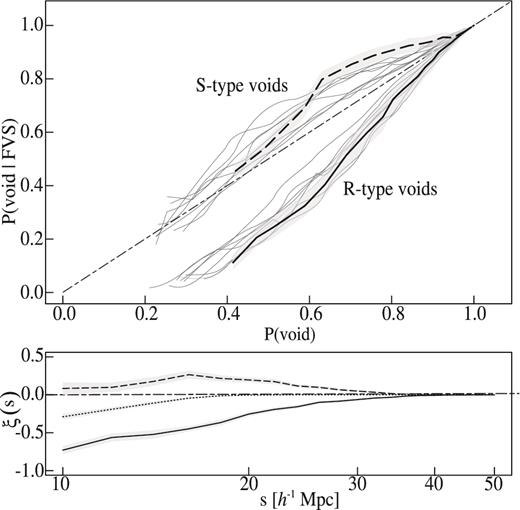
Spatial distribution of voids with respect to FVSs, in the SDSS data. Upper panel: conditional probability of finding a randomly placed sphere containing void and FVS volume fractions simultaneously; P(void | FVS) as a function of the probability that the same sphere contains a fraction of void volume P(void). The shaded regions indicate Jackknife resampling uncertainties. The grey curves correspond to random regions within the simulation with the same volume than SDSS sample. The bottom panel shows the corresponding void–FVS correlations in a similar way to Fig. 2.

Open in new tabDownload slide

In Fig. 9, we show the histograms of cos (θ) in four subsamples to show the effects of mass and distance to the closest FVSs. For reference, we show the corresponding values of the dipole moment |$\mathcal {D}$| which should be considered in the context of Fig. 5 that gives the same analysis in the simulation taking advantage of the larger statistics. In panel (a), we show voids located at a distance to the closest FVS, smaller than 60 per cent of the distance to the second closest FVS satisfying a total luminosity ratio of at least 0.6. These restrictions take into account the results shown in Fig. 5 for the simulation box and corresponds to the bottom-right corner, where the dipole moment signal has the larger amplitude. In this case, there is a clear prevalence of negative values of cos(θ), which is consistent with a negative value of the dipole moment. In panel (b), we show the histogram of cos(θ) for voids closer than 20 h⁻¹ Mpc to FVSs that have a total luminosity of at least 10¹³ L_⊙. Similarly to the previous subsample, this region is selected from the upper panel of Fig. 4 corresponding to the bottom-right corner of the plot. We also considered two additional restrictions corresponding to voids closer than 20 h⁻¹ Mpc to FVSs and a total luminosity up to 10¹³ L_⊙ (in panel (c) of Fig. 9) and to voids associated with luminous FVSs (L > 10¹³ L_⊙) separated by a distance greater than 30 h⁻¹ Mpc (panel (d)). This limiting mass was chosen so that the signal-to-noise ratio is high and taking into account the results in the simulation (Fig. 4) that indicates more massive FVSs have a more noticeable dipole moment. We argue that the infall patterns observed in the simulation box are also reproduced in the SDSS data despite its much smaller volume and the linearized velocity field approximation.

Figure 9.

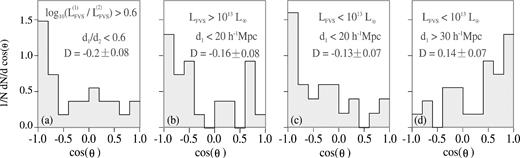
Histograms of the cos(θ) for different samples of voids in SDSS. (a) Voids that are at a distance to the closest FVS smaller than 60 per cent of the distance to the second closest FVS and also satisfying the ratio of the total luminosities of the two closest FVS >0.6, (b) voids closer than 20 h⁻¹ Mpc to FVSs having a total luminosity of at least 10¹³ L_⊙, (c) voids closer than 20 h⁻¹ Mpc to FVSs having a total luminosity up to 10¹³ L_⊙ and (d) voids near FVSs with L < 10¹³ L_⊙ separated by a distance greater than 30 h⁻¹ Mpc. We show the values of the dipole moments corresponding to each panel, with bootstrap resampling error estimates.

Open in new tabDownload slide

In the bottom panel of Fig. 7, we show the velocity pattern for the infall of galaxy groups in void shells on to FVSs. Our sample comprise 189 and 293 groups in R- and S-type void shells, respectively, in the 10–40 h⁻¹ Mpc galaxy–FVS distance range. The curves show the projected R–S velocity difference of groups in void shells on to the direction from the void centre to the FVS as a function of the location of the group. The angle ϕ between the relative position of the group and the FVS direction is as indicated in the scheme of Fig. 7. The dotted line is the resulting difference for the simulation. The solid line corresponds to SDSS data, with error bar indicating Jackknife resampling uncertainties. The region around the curve of the simulation gives an estimation of cosmic variance in order to compare the observations. It is computed from many randomly placed regions within the simulation with the same volume by using SDSS data and corresponds to a 2σ uncertainty.

5 DISCUSSION

In this work, we have explored the void–superstructure spatial cross-correlations and their influence on the large-scale velocity flows. To this end, we have studied the velocity field associated with galaxies in void shells to deepen our understanding of the supercluster–void network evolution.

Our void and superstructure catalogues are defined according to Ruiz et al. (2015) and Luparello et al. (2011), respectively. Therefore, voids correspond to spherical regions with an integrated total density of 10 percent and the mean value up to the void radius, and superstructures are derived from a smoothed luminosity field that isolates the highest density regions. These two definitions rely on physical grounds, namely the void sample has a constant integrated tracer density within void radii and superstructures correspond to future virialized systems in the accelerating Λ cold dark matter scenario.

In order to study the spatial correlations between voids and superstructures, we defined a modified version of the correlation which is usually applied to point data. This allows to measure the tendency of voids to be located at a given distance from a superstructure and detect if they are preferentially located near FVSs or avoiding them. We find that while voids-in-clouds (S-types) are preferentially located near superstructures, voids-in-voids (R-types) are likely to avoid them. This is somewhat related to the selection of voids according to their environment, but we find that it has also dynamical implications when considered in the context of the large-scale structure, manifested on the infall of voids which are close to FVS independently of void type.

We also explored galaxies in void shells and how the presence of a nearby superstructure affects its dynamics. Galaxies in S- and R-type void shells within 40 h⁻¹ Mpc infall on to superstructures except for galaxies opposite to superstructures in R-type void shells. Moreover, we find a stronger infall for galaxies residing in void shells facing the closest superstructure than galaxies at the same relative distance elsewhere. We have analysed the similarity of the simulation results and those inferred from the SDSS galaxy catalogue. In spite of the SDDS smaller observational volume and linear velocity approach and the fact that the Millenium simulation cosmological parameters differ from more recent observational estimates (Planck Collaboration et al. 2016), the general trend agreement is encouraging.

Large-scale flows may be analysed into different contexts (see for instance Shandarin 2011; Shandarin, Habib & Heitmann 2012; Cautun et al. 2014, and references therein). In our study, galaxy motions in void shells can be thought as a combination of shell expansion (Paz et al. 2013), void bulk motion (Lambas et al. 2016) and the infall on to superstructures (this work). The magnitude of these effects are comparable and need to be taken into account in simple models for galaxy motions. Our findings go along with the scenario proposed by Tully et al. (2008, 2014) where the presence of underdense regions significantly contribute to the velocity flow of galaxies in the local universe.

Acknowledgments

This work was partially supported by the Consejo Nacional de Investigaciones Científicas y Técnicas (CONICET) and the Secretaría de Ciencia y Tecnología, Universidad Nacional de Córdoba, Argentina.

Plots were made using r software and post-processed with Inkscape. This research has made use of NASA's Astrophysics Data System.

Funding for the SDSS and SDSS-II has been provided by the Alfred P. Sloan Foundation, Participating Institutions, National Science Foundation, US Department of Energy, National Aeronautics and Space Administration, Japanese Monbukagakusho, Max Planck Society and Higher Education Funding Council for England. The SDSS website is http://www.sdss.org/. The SDSS is managed by the Astrophysical Research Consortium for the Participating Institutions. The Participating Institutions are the American Museum of Natural History, Astrophysical Institute Potsdam, University of Basel, University of Cambridge, Case Western Reserve University, University of Chicago, Drexel University, Fermilab, Institute for Advanced Study, the Japan Participation Group, Johns Hopkins University, Joint Institute for Nuclear Astrophysics, Kavli Institute for Particle Astrophysics and Cosmology, Korean Scientist Group, Chinese Academy of Sciences (LAMOST), Los Alamos National Laboratory, Max-Planck-Institute for Astronomy (MPIA), Max-Planck-Institute for Astrophysics (MPA), New Mexico State University, Ohio State University, University of Pittsburgh, University of Portsmouth, Princeton University, United States Naval Observatory, and University of Washington.

REFERENCES