


Abstract
We present predictions of spectral energy distributions (SEDs), from the UV to the FIR, of simulated galaxies at z = 0. These were obtained by post-processing the results of an N-body+hydro simulation of a cosmological box of side 25 Mpc, which uses the Multi-Phase Particle Integrator (MUPPI) for star formation and stellar feedback, with the grasil-3d radiative transfer code that includes reprocessing of UV light by dust. Physical properties of our sample of ∼500 galaxies resemble observed ones, though with some tension at small and large stellar masses. Comparing predicted SEDs of simulated galaxies with different samples of local galaxies, we find that these resemble observed ones, when normalized at 3.6 μm. A comparison with the Herschel Reference Survey shows that the average SEDs of galaxies, divided in bins of star formation rate (SFR), are reproduced in shape and absolute normalization to within a factor of ∼2, while average SEDs of galaxies divided in bins of stellar mass show tensions that are an effect of the difference of simulated and observed galaxies in the stellar mass–SFR plane. We use our sample to investigate the correlation of IR luminosity in Spitzer and Herschel bands with several galaxy properties. SFR is the quantity that best correlates with IR light up to 160 μm, while at longer wavelengths better correlations are found with molecular mass and, at 500 μm, with dust mass. However, using the position of the FIR peak as a proxy for cold dust temperature, we assess that heating of cold dust is mostly determined by SFR, with stellar mass giving only a minor contribution. We finally show how our sample of simulated galaxies can be used as a guide to understand the physical properties and selection biases of observed samples.
1 INTRODUCTION
The current ΛCDM cosmological model is able to reproduce a number of fundamental observations, such as temperature fluctuations in the cosmic microwave background, Hubble diagram of distant supernovae, large-scale distribution of visible matter in the Universe, evolution of galaxy cluster abundances (e.g. Conroy, Wechsler & Kravtsov 2006; Springel, Frenk & White 2006; Vikhlinin et al. 2009; Betoule et al. 2014; Planck Collaboration XVI 2014). While this is the context in which galaxy formation takes place, a complete theory of galaxy formation continues to be elusive and our understanding of the physical processes that lead to the observed properties of galaxies is far from satisfactory (e.g. Silk & Mamon 2012; Primack 2015).
On the theoretical side, the problem of galaxy formation has been faced with the two main techniques of semi-analytic models and hydrodynamic simulations. This last technique has progressed rapidly thanks to the development of more sophisticated numerical algorithms and to the increasing computational power (e.g. Springel 2016). However, even the current computing power makes it impossible to resolve the wide range of scales needed to describe the formation of a galaxy in cosmological environment from first principles. As a consequence, processes like star formation, accretion of matter on to a supermassive black hole, and their energetic feedbacks, must be included into the code through suitable sub-resolution models. Early attempts to produce realistic galaxies, reviewed in Murante et al. (2015), were not successful due to a number of problems, the most important being the catastrophic loss of angular momentum. The Aquila comparison project (Scannapieco et al. 2012) demonstrated that at that time none of the tested codes was able to produce a really satisfactory spiral galaxy in a Milky-Way–sized dark matter halo with quiet merger history: most simulated galaxies tended to be too massive and too compact, with rotation curves sharply peaking at ∼5 kpc. It was suggested in that paper that the crucial process for a successful simulation is effective stellar feedback. That paper triggered a burst of efforts to improve sub-grid models in order to solve the discrepancies with observations. Different authors (e.g. Brook et al. 2012; Doménech-Moral et al. 2012; Aumer et al. 2013; Obreja et al. 2013; Stinson et al. 2013; Cen 2014; Hopkins et al. 2014; Vogelsberger et al. 2014; Schaye et al. 2015; Agertz & Kravtsov 2016; Marinacci, Pakmor & Springel 2016), using different codes, hydro scheme and sub-resolution models, are now able to produce late-type spiral galaxies with realistic properties: extended discs, flat rotation curves, low bulge-to-total ratios.
In Murante et al. (2015), our group presented cosmological simulations of individual disc galaxies, carried out with gadget3 (Springel 2005), including a novel sub-resolution model MUlti-Phase Particle Integrator (MUPPI) for star formation and stellar feedback. Using initial conditions of two Milky-Way–sized haloes (one being the Aquila Comparison halo), the paper presented late-type galaxies with properties in broad agreement with observations (disc size, mass surface density, rotation velocity, gas fraction) and with a bar pattern developing at very low redshift and likely due to marginal Toomre instability of discs (Goz et al. 2015). Simulations of small cosmological volumes of side 25 and 50 Mpc (H0 = 72 km s−1 Mpc−1), obtained using the same code of Murante et al. (2015), were presented in Barai et al. (2015). In that paper, the main properties of outflows generated by the feedback scheme (velocity, mass load, geometry) were investigated and quantified, showing broad agreement with observational evidence.
Simulations directly provide predictions on physical quantities like stellar masses, gas masses or star formation rates (SFRs), while most observed quantities are related to radiation emitted in given bands of the electromagnetic spectrum. Comparisons of model galaxies with observations can be carried out either by using physical quantities obtained from observations or by synthesizing observables from the simulation itself. While the first approach is easier to carry out once quantities like stellar masses, SFRs or gas masses are available for large samples of galaxies, it is clear that exploiting the full extent of panchromatic observations can produce much tighter constraints on models. Moreover, many assumptions on the stellar initial mass function (IMF), galaxy SFR history and dust attenuation are needed to infer physical quantities from observed ones, and these assumptions would better be made on the model side.
To properly synthesize observables from a simulation snapshot it is necessary to compute radiative transfer of starlight through a dusty interstellar medium (ISM), thus producing both attenuation of optical–UV light and re-emission in the FIR (see e.g. the recent review by Jones 2014). Observations across the electromagnetic spectrum reveal that galaxy spectral energy distributions (SEDs) strongly depend on the relative geometry of stars and dust, as well as on the properties of dust grains (e.g. Fritz et al. 2012). This complexity produces results that are not easily represented by simple approximations, as shown, e.g., by Fontanot et al. (2009a) even in the idealized case of semi-analytic galaxies where geometry is represented by a simple bulge/disc system.
It is only in recent years that the full SEDs of simulated galaxies have been studied, using different approaches to follow the transfer of radiation through the ISM and to calculate a global radiation field, and hence dust re-emission. Examples of codes for 3D radiative transfer are the following: sunrise (Jonsson, Groves & Cox 2010), skirt (Camps & Baes 2015), radishe (Chakrabarti & Whitney 2009), art2 (Li et al. 2008), all using Monte Carlo techniques and dart-ray (Natale et al. 2014), a ray-tracing code. Only few codes take into account structure on scales of star-forming regions, or include emission lines. sunrise includes the treatment of star-forming regions using the dust and photoionization code mappingsIII (Groves et al. 2008). The same approach is adopted by Camps et al. (2016) for particles in star-forming regions. Several authors have performed broad-band radiative transfer modelling for simulations of isolated or cosmological galaxies (Jonsson et al. 2010; Narayanan et al. 2010; Scannapieco et al. 2010; Hayward et al. 2011, 2012, 2013; Guidi, Scannapieco & Walcher 2015; Hayward & Smith 2015; Natale et al. 2015; Saftly et al. 2015).
In this work, we use the grasil-3d code (Domínguez-Tenreiro et al. 2014) to post-process a sample of 498 simulated galaxies obtained in a cosmological volume of side 25 Mpc presented by Barai et al. (2015). This code, based on grasil formalism (Silva et al. 1998), performs radiative transfer of starlight in an ISM that is divided into diffuse component (cirrus) and molecular clouds, which are treated separately on the ground that the molecular component is unresolved in such simulations. Therefore, in order to treat the very important dust reprocessing in molecular clouds, grasil-3d introduces a further sub-resolution modelling of these sites of star formation, on the lines of the original grasil. Other features inherited by the original code are a self-consistent computation of dust grain temperatures under the effect of UV radiation, re-emission of dust in the IR and a model of polycyclic aromatic hydrocarbons (PAHs). grasil-3d has been used to study the IR emission of simulated galaxies (Obreja et al. 2014) and galaxy clusters (Granato et al. 2015).
This paper is devoted to the study of panchromatic SEDs of our simulated galaxies at z = 0. The choice of redshift is motivated by the high quality of observations in the local Universe (Boselli et al. 2010; Gruppioni et al. 2013; Cook et al. 2014b,a; Clark et al. 2015; Groves et al. 2015), which allows a more thorough comparison. We will concentrate on the average SED of galaxies, trying to reproduce the selection of observed samples used for the comparison, and on the scaling relations of several basic quantities (like stellar mass, SFR, atomic and molecular gas masses, gas metallicities) among them and with FIR luminosity. As a result, we will show that, despite the existence of several points of tension with observations, the panchromatic properties of simulated galaxies resemble those of observed ones, to the extent that they can be used as a guide to understand the physical properties and selection biases of observed samples.
The paper is organized as follows. Section 2 presents the simulation code, the sub-resolution model used, the run performed, the grasil-3d code and the post-processing performed with it to produce SEDs for our galaxies. Section 3 presents the observational samples used for the comparison with data. Section 4 is devoted to the comparison of simulation results to observations. First, the global properties of the simulated sample at z = 0 are presented. Then average galaxy SEDs, in bins of stellar mass or SFR are shown to closely resemble observed ones. We then quantify the correlation of IR luminosities, from Spitzer to Herschel bands, with physical galaxy properties. Section 5 gives the conclusions.
2 SIMULATIONS
2.1 Simulation code
Simulations were performed with the Tree-PM+SPH gadget3 code, non-public evolution of gadget2 (Springel 2005). Gravity is solved with the Barnes & Hut (1986) Tree algorithm, aided by a Particle Mesh scheme on large scales. Hydrodynamics is integrated with an SPH solver that uses an explicitly entropy-conserving formulation with force symmetrization. No artificial conduction is used in this simulation (see e.g. Beck et al. 2016).
Star formation and stellar feedback are implemented using the sub-resolution model MUPPI, described in its latest features in Murante et al. (2015). Loosely following Monaco (2004), it is assumed that a gas particle undergoing star formation samples a multiphase ISM, composed of cold and hot phases in pressure equilibrium.
SN feedback is distributed in both thermal and kinetic forms, within a cone whose axis is aligned along the direction of the least resistance path (i.e. along the direction of minus the local density gradient) and within the particle's SPH smoothing length (see Murante et al. 2015 for full details). There is no active galactic nucleus (AGN) feedback in this version of the code.
Star formation is implemented with the stochastic model of Katz, Weinberg & Hernquist (1996) and Springel & Hernquist (2003), where a new star particle is spawned with a probability that depends on the stellar mass accumulated in one hydro time-step. Each star particle represents a simple stellar population (SSP) with a given IMF from Kroupa, Tout & Gilmore (1993) in the mass range (0.1–100) M⊙. Its chemical evolution is treated as in Tornatore et al. (2007): the stellar mass of the particle is followed since its birth (spawning) time, accounting for the death of stars and stellar mass-losses. The code tracks the production of different species: He, C, Ca, O, N, Ne, Mg, S, Si, Fe and a further component of generic ‘ejecta' containing all other metals. It takes into account yields from type Ia SNe (Thielemann et al. 2003), type II SNe (Chieffi & Limongi 2004) and asymptotic giant branch (AGB) stars (Karakas 2010). Such mass-losses are distributed to neighbouring gas particles together with the newly produced metals. The yields we use in this simulation are updated with respect to Barai et al. (2015). Radiative cooling is implemented by adopting cooling rates from the tables of Wiersma et al. (2009), which include metal-line cooling by the above-mentioned chemical elements, heated by a spatially uniform, time-dependent photoionizing background (Haardt & Madau 2001). Gas is assumed to be dust-free, optically thin and in (photo)ionization equilibrium.
2.2 SED synthesis with grasil-3d
Domínguez-Tenreiro et al. (2014) presented the radiative transfer code grasil-3d that post-processes the output of a simulation to synthesize the panchromatic SED of the galaxy. It is based on the widely employed GRASIL (GRAphite and SILicate) model (Silva et al. 1998; Silva 1999; Granato et al. 2000), which self-consistently computes the radiation field of a galaxy, emitted by stars and attenuated by dust, and the temperature of dust grains heated by the radiation itself. While the original code was applied to galaxies composed of idealized bulge and disc components, grasil-3d is applied to the arbitrary geometry of a simulated distribution of star particles. We refer the reader to the Domínguez-Tenreiro et al. (2014) paper for an exhaustive discussion of this code. Its main features are summarized below, focusing on the few modifications that we introduced to interface it with the output of our version of gadget3.
grasil-3d treats the ISM as divided into two components: optically thick molecular clouds (hereafter MCs), where stars are assumed to spend the first part of their life, and a more diffuse cirrus component. This separation, which is well founded in the observed properties of young stars, produces an age-selective dust extinction, with the youngest and most UV-luminous stars suffering the largest extinction. The physical quantity that regulates this division is the escape time tesc of stars out of the MC component. Inside MCs, starlight is subject to an optical depth τ ∝ δΣMC that is proportional to the cloud surface density ΣMC. Both the original grasil code and grasil-3d require two parameters to describe MCs (assumed to be spherical): their mass MMC and their radius RMC. However, all the results depends only on their surface density, which is a combination of the two parameters: |$\Sigma _{\rm {MC}} = M_{\rm MC}/R_{\rm MC}^2$| (see Silva et al. 1998 for details). In the following, we will use the MC mass as a free parameter, while keeping RMC fixed at 15 pc, a rather typical value for Galactic giant molecular clouds. We stress that the specific value of this parameter is immaterial, it only determines the relation between MC mass and surface density.
Gas and stellar mass densities are constructed by smoothing particles on a Cartesian grid, whose cell size is set by the force softening of the simulation. For gas mass, we used cold (T < 105 K) and multiphase gas particles. The original code uses a sub-resolution model to estimate the molecular fraction of a gas particle. A different strategy is applied in our case, where the molecular gas mass is computed by MUPPI using equation (1).
However, the stochastic star formation algorithm does not guarantee that molecular gas is associated with the youngest stars, so the association of star particles with MCs, a working assumption of grasil-3d, is subject to unphysical fluctuations.
We modified grasil-3d to read molecular fraction of gas particles directly from the simulation output. Atomic gas is simply identified with the cirrus component. For the MC component, grasil-3d computes the density of stars younger than tesc, then redistribute the molecular mass proportionally to that density, so as to guarantee perfect coincidence of the two components. To compute unattenuated starlight, we adopt a Chabrier (2003) IMF. The version of grasil-3D used in this paper is based on models of simple stellar populations (SSPs) by Bruzual & Charlot (2003), so we could not simply replicate the choice of Kroupa et al. (1993) made in the simulation. But the two IMFs are so similar that we do not expect this difference to have any impact on the results.
Dust is assumed to consist of a mixture of silicates and graphites, where the smaller carbonaceous grains, with size lower than 100 Å, are assumed to have PAH properties (either neutral or ionized). The dust model used for the diffuse cirrus is that proposed by Weingartner & Draine (2001); Draine & Li (2001); Li & Draine (2001), updated by Draine & Li (2007), a model originally calibrated to match the extinction and emissivity properties of the local ISM. For small grains, use has been made of the MW3.1_60 model in table 3 of Draine & Li (2007), with a PAH-dust mass fraction q_PAH = 4.58 (i.e. the Galactic value around the Sun). This q_PAH value is also consistent with observational data for other normal galaxies (i.e. no low-metallicity ones), as can be seen, for example, in Draine et al. (2007, fig . 20) and Galliano et al. (2008, figs 25 and 29). The PAH ionization fraction has also been taken from Draine & Li (2007). This model is similar to the BARE-GR-S model introduced by Zubko, Dwek & Arendt (2004). For MCs, the original mixture used by Silva et al. (1998) is assumed, calibrated against the local ISM and later on updated to fit the MIR emissions of a sample of actively star-forming galaxies by Dale et al. (2000, see Vega et al. 2005, 2008 for more details). In particular, PAH in MCs have been depleted by a factor of 1000 relative to their abundance in the diffuse component.
In this paper, we refer to original papers for a justification of the assumptions made in the dust model choice, and make no attempt to test the effects of changes in dust parameters, with the exception of dust emissivity index β. In fact, in Appendix A3, we test the results of changing this canonical value β = 2 adopted here and the recent determination of β = 1.62 ± 0.10 (Planck Collaboration XVI 2014). This affects the sub-mm side of the SEDs but does not greatly affect the conclusions presented here.
While dust mass and molecular fraction are fixed by the simulation as explained above, two parameters need to be decided, namely the escape time tesc and τ (the latter being represented by variations of MC mass MMC at fixed radius RMC of 15 pc). In Appendix B, we show the robustness of resulting SEDs to variations of these parameters around their reference values. Finally, in Appendix A1, we test the stability of results to the exact choice of grid size, and on the choice of aperture to define which particles belong to the galaxy.
2.3 Simulation run
The simulation, called MUPPIBOX in this paper, represents a cosmological periodic volume of Lbox = 25 comoving Mpc (H0 = 72 km s−1 Mpc−1), sampled by Npart = 2563 DM particles and as many gas particles in the initial conditions. Initial gas particle mass is mgas = 5.36 × 10⁶ M⊙. The Plummer-equivalent softening length for gravitational forces is set to Lsoft = 2.08 comoving kpc up to z = 2, then it is held fixed at Lsoft = 0.69 kpc in physical units from z = 2 up to z = 0. The simulation is very similar to the M25std presented in Barai et al. (2015), but with improved yields and slightly different parameters for the MUPPI sector, to absorb the differences induced in the cooling rate by the different metal compositions: fb, out = 0.2, fb, kin = 0.5, Pkin = 0.02.
To select galaxies, we proceed as in Murante et al. (2015) and Barai et al. (2015). The simulation is post-processed with a standard friends-of-friends algorithm and with the substructure-finding code SubFind (Springel et al. 2001) to select main haloes and their substructures. Galaxies are associated with substructures (including the main haloes), their centre is defined using the position of the most bound particle. Star and cold (T < 105 K) or multiphase gas particles that stay within a fiducial distance Rgal = 0.1Rvir (a tenth of the virial radius of the host main halo) constitute the visible part of the galaxy; they will be named galaxy particles in the following. The reference frame of each object is aligned with the inertia tensor of all galaxy particles within a fiducial distance of 8 kpc from the galaxy centre, to avoid misalignments due to close galaxies. The Z-axis is aligned with the eigenvector corresponding to the largest eigenvalue of the inertia tensor and on the direction of the star angular momentum, while the other axes are aligned with the other eigenvectors so as to preserve the property |$\hat{X} \times \hat{Y} = \hat{Z}$|. Whenever a disc component is present, aligning with the inertia tensor is equivalent to aligning the Z-axis with the angular momentum of stars.
Galaxy morphologies are simply quantified through the B/T, bulge-over-total ratio. Star particle circularities are defined as |$\epsilon = J_{z}/J\rm _{circ}$|, where Jz is the specific angular momentum along Z-axis, and |$J_{{\rm circ}} = r\sqrt{(GM(<r))/r}$| angular momentum of a circular orbit at the same distance. The bulge mass is estimated as twice the mass of counter-rotating particles, the disc mass is assumed to be the remaining stellar mass. This simple procedure is known to overestimate B/T with respect to fitting a synthetic image of the galaxy, reproducing the procedure performed by observers (Scannapieco et al. 2010). Other bulge definitions and mass measurements are possible (see e.g. Doménech-Moral et al. 2012; Obreja et al. 2013).
We consider galaxies with stellar mass >2 × 10⁹ M⊙ within |$R\rm _{gal}$|. This way each object is resolved with at least ≃ 2 × 10³ star particles. Below this mass, the stellar mass function is observed to drop, so this is a conservative estimate of the completeness limit mass of the simulation. With this selection, the sample amounts to 498 objects. All quantities (masses, luminosities, etc.) are computed on galaxy particles within Rgal; in Appendix A2, we discuss how galaxy SEDs change when we adopt another definition of aperture radius, inspired by the Petrosian radius (Petrosian 1976). SEDs do depend on galaxy inclination, so they were not computed using the reference frame aligned with the galaxy inertia tensor, but in a frame aligned with the box reference frame. This way the line of sight is along the Z-axis of our box, yielding an essentially random orientation for each galaxy.
3 OBSERVATIONAL SAMPLES USED FOR THE COMPARISON
We want to compare predicted SEDs of simulated galaxies to pan-chromatic observations of local galaxies. To this aim, we have selected observational samples that provide SEDs as well as recovered physical properties of observed galaxies (stellar masses, SFRs, gas and dust masses, etc.).
A first step in the analysis consists in the comparison of overall SED shapes, once a common normalization is adopted. This is done by grouping galaxies in bins of stellar mass and comparing the median of their predicted near-UV to far-IR SEDs with the results of two local samples, namely Local Volume Legacy (LVL; Cook et al. 2014a,b) and PACS Evolutionary Probe (PEP; Gruppioni et al. 2013). In this comparison, all SEDs will be normalized to the 3.6 μm flux, so the test will only be sensitive to the overall SED shape and not to its normalization. The IR part of SEDs will then be compared to the results of the Herschel Reference Survey (HRS) of Boselli et al. (2010), by grouping galaxies according to several physical quantities. Finally, tests of scaling relations of physical properties (gas and dust mass) and observable properties (FIR luminosity) will be performed using the Herschel-ATLAS Phase-1 Limited-Extent Spatial Survey (HAPLESS) sample (Clark et al. 2015) and the sample by Groves et al. (2015). These samples are described below.
To be consistent with the adopted stellar mass threshold of simulated galaxies, we will always select observed galaxies above a stellar mass limit of 2 × 10⁹ M⊙.
3.1 LVL sample
LVL (Cook et al. 2014a,b) consists of 258 nearby galaxies (D ≤ 11 Mpc), considered as a volume-limited, statistically complete and representative sample of the local Universe. Galaxies are selected with mB < 15.5 mag (Dale et al. 2009) and they span a wide range in morphological type, but clearly the sample is dominated by dwarf galaxies due to its volume-limited nature. LVL SEDs cover the range from GALEX FUV band to Herschel MIPS160 band. Physical properties like stellar mass and SFRs have been obtained through SED fitting techniques, we refer to the original papers for all details.
3.2 PEP sample
PEP (Gruppioni et al. 2013) is a Herschel survey that covers the most popular and widely studied extragalactic deep fields: COSMOS, Lockman Hole, EGS and ECDFS, GOODS-N and GOODS-S (see Berta et al. 2010; Lutz et al. 2011, for a full description). Galaxies are selected with flux densities ≥5.0 and ≥10.2 mJy at 100 and 160 μm, respectively. SEDs cover the range from U-band to SPIRE500 Herschel band. Being interested in the local Universe, we selected galaxies with z < 0.1. Physical properties of PEP galaxies are obtained with SED fitting technique using magphys (da Cunha, Charlot & Elbaz 2008). This code uses a Bayesian approach to find, at a given redshift, the template that best reproduces the observed galaxy fluxes. We use spectroscopic redshifts provided by PEP for all galaxies in our sample. SED templates are obtained from libraries of stellar population synthesis models of Bruzual & Charlot (2003) with a Chabrier (2003) IMF and a metallicity value that can be in the range of 0.02–2 Z⊙. As for the SFR history, magphys assumes an exponentially declining (SFR ∝ exp (−γt)) to which random bursts are superimposed. The probability distribution function of the star formation time-scale is p(γ) = 1 − tanh (8γ − 6), which is uniform between 0 and 0.6 Gyr−1 and then drops exponentially to zero at 1 Gyr−1. The age of the galaxy is another free parameter, with an upper limit provided by the age of the Universe at the chosen redshift. The code outputs probability distribution functions of physical parameter values (stellar mass, SFR) that give best-fitting SEDs. We adopt median values, which are a more robust estimator, while the 1σ uncertainty is given by half of the difference between the 16th and 84th percentiles.
3.3 HRS sample
HRS (Boselli et al. 2010) is a volume-limited sample selected between 15 and 25 Mpc (H0 = 70 km s−1 Mpc−1), complete for K ≤ 12 (total Vega magnitude) for late types and K < 8.7 for early types. For the late types, this corresponds to a stellar mass limit of ∼109 M⊙, smaller than our limit by a factor of ∼2. It contains 322 galaxies, 62 early-types and 260 late-types. IR SEDs of the HRS galaxies range from 8 to 500 μm, where MIR photometry is obtained by Spitzer/IRAC and WISE images plus archival data from Spitzer/MIPS, and FIR photometries are obtained from Herschel/PACS, Herschel/SPIRE and IRAS (Ciesla et al. 2014). We used HRS infrared SED templates available to the community via the HEDAM1 website.
3.4 HAPLESS sample
HAPLESS (Clark et al. 2015) consists of 42 nearby galaxies (15 < D < 46 Mpc), taken from the H-ATLAS Survey. The sample spans a range of stellar mass from 7.4 to 11.3 in log M⋆, with a peak at 108.5 M⊙, and specific SFR from −11.8 to −8.9 in log yr−1. Most galaxies have late-type, irregular morphology. HAPLESS provides masses and temperatures of cold and warm dust for its galaxies, obtained by fitting two modified blackbodies to the FIR SEDs.
3.5 Groves sample
Groves et al. (2015) presented a sample collected from KINGFISH (Herschel IR), HERACLES (IRAM CO) and THINGS (VLA HI) surveys (Walter et al. 2008; Leroy et al. 2009; Kennicutt et al. 2011). The matched data sets give 36 nearby galaxies with average distance of 10 Mpc, ranging from dwarf galaxies to massive spirals, that are dominated by late-type and irregular galaxies. Stellar masses span the range from 106.5 to 1010.5 M⊙, with a median log M⋆/M⊙ of 9.67. SFRs cover approximately 4 orders of magnitudes from 10−3 to 8 M⊙ yr−1.
4 COMPARISON OF SIMULATED AND OBSERVED GALAXY SAMPLES
4.1 Global properties of the simulated sample
We start from showing the range of variation of the main galaxy physical properties, that is necessary to assess the statistical properties of the sample. Fig. 1 shows the stellar mass, atomic, molecular and total gas masses, dust masses and B/T distributions of the 498 simulated galaxies at z = 0. From the histograms, we find that ≃80 per cent of the sample is composed of galaxies with total stellar mass lower than 1010 M⊙, and ≃ 90 per cent of the atomic and molecular hydrogen is locked in those galaxies. The median value for dust mass is |${\rm {\rm l}og} (M\rm {_{dust}}/{\rm M}_{\odot }) \simeq 7$| and for B/T ∼ 0.5.

Distribution of the main physical properties of simulated galaxies. From left to right, and from top to bottom: stellar mass M⋆, total (cold and multiphase) gas mass Mgas, atomic gas mass |$M_{{\rm H\,\small {i}}}$|, molecular gas mass |$M_{{\rm H}_2}$|, dust mass Mdust and bulge-to-total ratio B/T.
The range of values for these physical properties is realistic, but there are a few points of tension with observations: the stellar mass function is steeper than the observed one, though the statistics is poor to assess the significance of this disagreement; the few massive galaxies (M★ > 3 × 10¹⁰ M⊙) present in this volume tend to be star-forming and with low B/T, and this can be ascribed to the lack of AGN feedback in this code implementation.
To compare SFRs with observations, we should take into account the range of stellar ages to which the SFR indicators used are sensitive, with values going from a few to ≈100 Myr (e.g. Kennicutt 1998; Calzetti et al. 2005; Calzetti 2013). There are two ways to recover SFRs of simulated galaxies. One can take the instantaneous SFR produced by the sub-resolution model at the output time, or one can consider the number of star particles spawned by the stochastic star formation algorithm in a given time interval. To give an example, at the resolution of our simulation an SFR of 1 M⊙ yr−1 will produce one star particle of 1.34 × 10⁶ M⊙ each 1.34 Myr. As a consequence, a proper average of SFR would require a time of order ∼100 Myr to properly suppress shot noise, the problem being more severe at lower SFRs. We have verified that the instantaneous and averaged SFRs show a very good correlation, with a scatter that increases with decreasing age intervals used for the average SFR. For this reason we use the largest age interval of 100 Myr to compute average SFRs, with the caveat that some indicators may be sensitive to smaller age intervals.
In Fig. 2, we show how well the physical properties of our simulated galaxies resemble observed ones. It is clear that this comparison is not completely consistent, because the quantities extracted from observations and simulations are subject to different selection criteria; comparisons in terms of observables will be presented later. The upper-left panel of Fig. 2 shows the main sequence of star-forming simulated galaxies (e.g. Elbaz et al. 2007, 2011; Noeske et al. 2007; Peng et al. 2010) for the MUPPIBOX sample. This has been obtained by a linear regression, performed with the robust method of Cappellari et al. (2013), of the simulated galaxies in the (log–log) M⋆ − SFR plane, shown as grey points. The fit is reported as a blue line, the shaded area gives the 1σ error on the normalization. The scatter of simulated galaxies around the main sequence is of order of 0.3 dex, compatible with observations. The same fitting procedure has been applied to the LVL, PEP, Groves and HAPLESS samples that are reported in the same figure (in this case we do not show the single galaxies). In the figure, we also report the fit to the main sequence measured in the HRS sample as a black line; in this case, we do not show an uncertainty on the relation. The lower sub-panel shows the residuals of simulated galaxies with respect to the mean relation as a function of the galaxy B/T. This is shown to highlight possible dependencies on galaxy morphology; in this case, we obtain that early-type galaxies tend to stay below the relation, as expected. The figure shows an overall consistency of the main sequence of star-forming galaxies between simulations and observations. The simulated relation is however steeper than that found in some of the samples, especially the HRS one, and this leads to some disagreement above 1010 M⊙. Indeed, all simulated galaxies in the sample have significant SFR, no passive galaxy is found even at high masses. This excess of star formation is a likely effect of the lack of AGN feedback in this simulation. At the same time, the least massive galaxies tend to be below the main sequence of observations (with the exception of LVL survey) by ∼0.5 dex, a typical behaviour of dwarf galaxies in a LCDM model (Fontanot et al. 2009b; Weinmann et al. 2012).
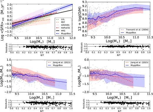
Upper-left panels: main sequences, in the M⋆ − SFR plane, of star-forming galaxies. For LVL, PEP, Groves and HAPLESS samples, and for the MUPPIBOX simulated sample, main sequences were obtained by a linear regression (in the log–log plane) using the robust estimator of Cappellari et al. (2013). The plot reports the obtained regression as a line and the error on its normalization as a shaded area. The black line marks the HRS fit, that has been provided by Ciesla et al. (2014). Simulated galaxies are shown in the background as grey points. The lower sub-panel, in this and all other figures, gives for the MUPPIBOX sample the residual of each galaxy with respect to the main relation as a function of B/T; this is given to highlight possible dependencies on galaxy morphology. Upper right panels: distribution of galaxies in the M⋆ − 12 + log (O/H) plane. Grey points give simulated galaxies, dashed red and solid blue lines show the median value of Tremonti et al. (2004) and of the MUPPIBOX sample, filled regions contain 68 per cent of the data (16th and 84th percentiles). Lower panels: distribution of galaxies in the |$M_{{\rm H\small {\,i}}}/M_\star -M_\star$| (left) or |$M_{{\rm H}_2}/M_\star -M_\star$| (right) plane. Grey points give simulated galaxies, dashed red and solid blue lines show the median value of Jiang et al. (2015), obtained using SMT, AMIGA-CO and COLD GASS samples, and of the MUPPIBOX sample, filled regions contain 68 per cent of the data (16th and 84th percentiles).
The upper right panel of Fig. 2 shows the gas metallicity of simulated galaxies as a function of M⋆. We also report as a continuous line the median values in bins of stellar mass chosen so as contain 30 galaxies, while the shaded area gives the 16th and 84th percentiles. A similar style is used to report the observational determination of Tremonti et al. (2004), relative to SDSS galaxies at z ∼ 0.1. For simulated galaxies, to derive the oxygen abundance we compute the mass-weighted average of oxygen mass of galaxy gas particles, and recast it in terms of O/H, assuming a solar value of 8.69 (Allende Prieto, Lambert & Asplund 2001). Simulated galaxies show the same trend as observations of increasing metallicity at larger stellar mass, but we find a global offset of ∼0.1 dex. At large stellar masses (M⋆ ≳ 1011 M⊙), this is likely due to the lack of quenching of cooling and star formation by AGN feedback, while the offset is much less evident at the 1010 M⊙ mass scale (apart from a few high-metallicity outliers). Metallicities are offset by up to 0.2 dex in the low-mass end of this relation. The lower sub-panel shows again the residuals of simulated galaxies with respect to the mean relation as a function of the galaxy B/T; no trend is visible in this case.
Next, we consider the abundance of atomic and molecular gas, as a function of stellar mass. We compare this to the determination of Jiang et al. (2015), who combined the STM (Groves et al. 2015), AMIGA-CO (Lisenfeld et al. 2011) and COLD GASS (Saintonge et al. 2011; Catinella et al. 2012) surveys. The lower panels of Fig. 2 show the location of simulated galaxies in the |$M_{{\rm H\,\small {i}}}/M_\star -M_\star$| (left-hand panel) and |$M_{{\rm H}_2}/M_\star -M_\star$| (right-hand panel) planes. As for the other panels of the same figure, we show simulated galaxies as grey dots, and the average of the simulated (same binning as for the stellar mass–gas metallicity relation) and observed relations with 16th and 68th percentiles denoted as a shaded area. Lower panels show again residuals of simulated galaxies versus B/T. Besides a broadly good agreement in the stellar mass range from 1010 to 1010.5 M⊙, atomic gas tends to be low in simulated galaxies, especially at small stellar masses, where the relation flattens and the mass ratio saturates at unity values, at variance with the observed relation. The relation with molecular gas is reproduced in a much better way, with some possible average overestimate. Looking at residuals, we notice that many outliers with low gas masses have early type morphologies; these objects may be absent in the observed sample due to selection. Following Jiang et al. (2015), we computed Spearman's correlation coefficients for these correlations, obtaining values of −0.40 for |${\rm H\,\small {i}}$| and −0.23 for H2, to be compared with −0.72 and −0.48 given in that paper.
This analysis shows that the simulated galaxy sample provides objects with properties that are broadly consistent with observations. This is in line with the findings of other simulation projects, like the Illustris (Vogelsberger et al. 2014) and EAGLE simulation (Schaye et al. 2015), where good agreement of simulated galaxies with observations at z = 0 extends to molecular and atomic gas, obtained in post-processing (Genel et al. 2014; Lagos et al. 2015; Bahé et al. 2016). However, our massive galaxies show a lack of proper quenching and small galaxies are too massive, passive, metallic and with low atomic gas content.
4.2 Average SEDs from UV to FIR
As explained in Section 2.2, radiative transfer in a dusty medium, performed by grasil-3d, requires to specify the escape time of stars from MCs, tesc, and the MC optical depth through their putative mass MMC (this enters in the computation only through MC mass surface density, and |$R\rm _{MC}$| is fixed to 15 pc). It has been shown several times (Silva et al. 1998; Granato et al. 2000, 2015) that GRASIL is able to reproduce normal star-forming galaxies at low redshift by assuming tesc in the range of 2–5 Myr and RMC ∼ 15 pc for an MMC = 106 M⊙ cloud. We thus adopt tesc = 3 Myr and MMC = 106 M⊙. In order to assess the impact of variations of these parameters on the resulting SEDs, we proceed as follows. We compute galaxy SEDs using tesc = 2, 3, 4 and 5 Myr, and MMC = 105, 106 and 107 M⊙. We divide the sample into three bins of stellar mass: 9.3–9.5, 9.5–10 and 10–10.5 in |${\rm {\rm l}og} \,M_\star /{\rm M}_{\odot }$|, excluding the few most massive galaxies that are affected by lack of quenching. For each mass bin and for each choice of the two parameters, we compute average SEDs, and compare them with the average SED of LVL and PEP samples, subject to the same mass limit. Details of these analyses are reported in Appendix B. This analysis shows that results are rather robust for variations of MMC, while tesc has a sizable effect in the MIR and, to a lesser extent, in the FUV. The adopted values give very good results in many mass bins, confirming their validity.
Having set grasil-3d parameters, we can now address the agreement of predicted galaxy SEDs with observed ones. In order focus on SED shapes, we perform this comparison by normalizing all the λLλ SEDs to their value at the 3.6 μm Spitzer/IRAC1 band, where the emission is dominated by old stars. As an alternative choice, we normalized the SEDs to their total FIR luminosity, integrated from 8 to 1000 μm. With respect to the first choice, the resulting SEDs showed, as expected a lower scatter in the FIR, compensated by some scatter at 3.6 μm. With these two normalization choices, we checked that average SEDs show the same qualitative trends versus other parameters; we will show in the following results obtained with the first choice.
Fig. 3 shows the average, normalized SED of galaxies in the simulated sample, compared with the median LVL and PEP SEDs. The number of objects is reported in each panel. Coloured areas give the scatter in the observed SEDs, quantified by the 16th and 84th percentiles. The four panels give the average SED for the whole sample (upper-left panel) and for three bins of stellar mass, as indicated above each panel. The LVL and PEP samples are selected in a different way, based on optical or FIR observations in the two cases and their SEDs show some differences, though they are generally compatible within their scatter. The agreement of simulated and observed SEDs is very good at all stellar masses. In the upper-left panel, the median SED of simulated galaxies lies always between the two observational medians. Even the PAH region is found within the observed range, while some underestimate is appreciable in the FUV, though the median curve is still within the 1σ observed range. Considering the average SEDs in bins of stellar mass, tension is visible in the smallest stellar mass bin; this is the stellar mass range for which discrepancies with observations were noticed in Section 4.1. Here, the average SED is underestimated in the range from 30 to 100 μm and in the UV, where it lies on the 16th percentile. The agreement is much better in the two higher mass bins: some underestimation in the UV bands is still present in the middle stellar mass bin, while the galaxies in the most massive stellar mass bin agree very well with observation, with only some overestimation limited to ∼ 20-30 μm, a range that is very sensitive to the exact value of the tesc parameter (see Appendix B).

Median SEDs (λLλ) of galaxies with M⋆ > 2 × 10⁹ M⊙ (upper-left panel) and in three bins of stellar mass as indicated above each panel, normalized to unity at the 3.6 μm IRAC1 band. Blue continuous line: simulated galaxy SEDs, obtained with grasil-3d using best-fitting parameters tesc = 3 Myr, and MMC = 106 M⊙. They are compared with the median SED of LVL (dot–dashed purple line) and PEP (dashed orange line) samples. Coloured areas give their 1σ uncertainty, obtained using the 16th and 84th percentiles. Every plot reports the number of galaxies in the MUPPIBOX, PEP and LVL samples.
To understand the origin of the underestimation of UV light, we address the FUV − Ks colour and correlate it with galaxy gas richness |$M_{{\rm H\,\small {i}}}/M_\star$| and metallicity to understand whether FUV reddening is caused by unproper SED synthesis or simply by the higher metallicities of galaxies of low mass. Because the LVL sample does not provide gas or dust masses, we use the HAPLESS sample; we restrict ourselves to |${\rm H\,\small {i}}$| gas mass because HAPLESS does not give molecular masses, and we use |$M_{\rm dust}/M_{\rm H\,{\rm \small {i}}}$| as a proxy for metallicity. Fig. 4 shows that observed and simulated galaxies lie on the same broad relation of FUV − Ks versus gas richness |$M_{{\rm H\,\small {i}}}/M_\star$|, with galaxies with lower metallicities being in general more gas-rich and less attenuated. The figure also reports the Spearman correlation coefficient for the two relations, for MUPPIBOX (cS) and HAPLESS (cO) galaxies, that turn out to be very similar. This test shows that the same FUV − Ks colours are obtained for galaxies with the same gas richness, so the difference in the average SEDs is induced by physical differences in input galaxy properties.
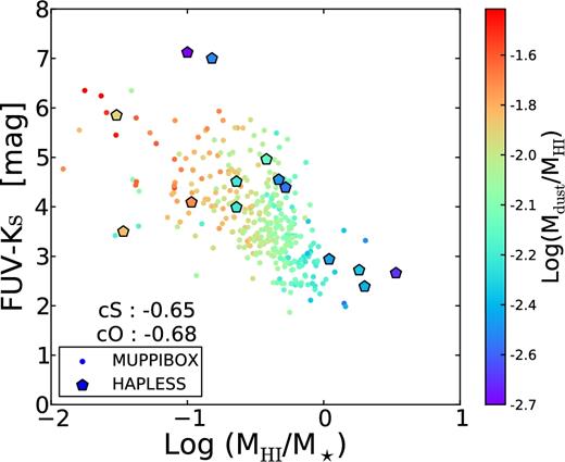
FUV − Ks colour versus gas fraction |$M_{{\rm H\,\small {i}}}/M_\star$|; points are colour-coded with |$M_{\rm dust}/M_{\rm {\rm H\small {\,i}}}$|. cS and cO show the Spearman coefficients for MUPPIBOX and HAPLESS samples, respectively.
We further test our SEDs in the range from 8 to 1000 μm by comparing them to the highly complete HRS sample, this time checking SED normalizations and not only their shapes. For this comparison, we use the results of Ciesla et al. (2014), who computed average SEDs for subsamples binned by stellar mass, SFR, dust mass, metallicity and morphological type. We show here results for bins in stellar mass and SFR; we recall that the stellar mass limit of HRS is ∼109 M⊙, a factor of ∼2 lower than our resolution limit, so the comparison with SEDs binned in stellar mass will be limited to M⋆ > 2 × 10⁹ M⊙, while the lower SFR bins will be affected by this mild mismatch in limiting mass. Fig. 5 shows the average SEDs for three bins of stellar mass (upper panels) and of SFR (lower panels); sample definition is given above each panel. Here, the blue continuous line gives the median SED of the simulated sample; this time we report the scatter of simulated galaxies, computed using the 16th and 84th percentiles. HRS SEDs are given by red dashed lines; Ciesla et al. (2014) do not give scatter for their SEDs. The comparison in bins of stellar mass (upper row of panels in the figure) confirms the trend of Fig. 2 of an underestimate of SFR (and thus of IR luminosity) for small galaxies: the normalization at the FIR peak is down by a factor of three for the smallest galaxies (from 9.5 to 10 in |${\rm {\rm l}og} \,M_\star /{\rm M}_{\odot }$|), of two for the intermediate mass bin (from 10 to 10.5), while a modest overestimate is present for the largest galaxies. SED shapes are very similar to the observed ones, peak positions are closely reproduced with the exception of the smallest galaxies where dust is colder; we will show below that this is a consequence of the lower level of star formation. The scatter of model galaxies, which was not shown in Fig. 3 for sake of clarity, is somewhat higher than what found in observations, especially at smaller masses.
![Comparison between median SEDs of simulated galaxy sample (blue continuous lines) and HRS (red dashed lines) for galaxies in various bins of stellar mass (first row) or SFR (second row). The blue filled region marks the 1σ uncertainty of the simulated sample, defined by the 16th and 84th percentiles. Above each panel we report the selection criterion used to define the subsample, while the number of simulated galaxies (MUPPI [number]) is reported in each figure.](https://oup.silverchair-cdn.com/oup/backfile/Content_public/Journal/mnras/469/4/10.1093_mnras_stx869/1/m_stx869fig5.jpeg?Expires=1750498713&Signature=BEqw~703jWyCP6nuDeXgyaGuw~yz2gYIfRAxnU3UjHqOCWsN3k913X0eGdLR2-rAAIso663gyNhxSysTR52~TdlGXkIdtHonIQERB5KvjqkrPegLSSGPF2xz8gCoZC22ahdP~WHc4-ZVAP5NOqPeSlLGZRDjQHLfXlOHiiNa1puGnSOny09w9LRw7su3LBIzBTrYUQRuOt5bP13QL5PGLQownsD-tjiIMbB51TcLtpgHryoiXj6bvMlxrDqW1tW8FZ8hUWdvoD5ZqcklBa2NtXU4prWHXVHxN2tYXgNNUunk2tWJdYkqmC-zwcC7fvKn4tx6Fkfs6kDC1qfHzFLoUg__&Key-Pair-Id=APKAIE5G5CRDK6RD3PGA)
Comparison between median SEDs of simulated galaxy sample (blue continuous lines) and HRS (red dashed lines) for galaxies in various bins of stellar mass (first row) or SFR (second row). The blue filled region marks the 1σ uncertainty of the simulated sample, defined by the 16th and 84th percentiles. Above each panel we report the selection criterion used to define the subsample, while the number of simulated galaxies (MUPPI [number]) is reported in each figure.
When galaxies are divided in bins of SFR (the second row in Fig. 5) differences in normalization are much lower, while the change in SED shape is broadly reproduced by grasil-3d. This shows that SFR is the main driver of IR light. The galaxies with lowest SFR are those where the agreement is worst, but this is the bin that is most populated by the smallest galaxies and most affected by the different stellar mass limit. We also find that scatter is dominated by galaxies with low SFR.
4.3 Correlation of IR luminosity with galaxy physical properties
After having quantified the level of agreement of simulated SEDs with observations, we consider here the correlation of IR/sub-mm luminosity with global properties of MUPPIBOX galaxies. This is done to understand to which physical quantity IR light is most sensitive, and which bands best trace that given quantity. We consider here bands from 3.6 to 500 μm, covering Spitzer and Herschel ones plus a fine sampling of the MIR region from 8 to 24 μm. For each simulated galaxy, we compute its luminosity and correlate it with atomic gas mass |$M_{{\rm H\small {\,i}}}$|, molecular gas mass |$M_{{\rm H}_2}$|, SFR, dust mass Mdust and stellar mass M⋆.
These quantities are of course all strongly correlated among themselves, so they will all correlate with IR luminosity. For each correlation, we compute Spearman and Pearson correlation coefficients, since they show the same behaviour, we restrict ourselves to the Spearman one. Fig. 6 shows these correlation coefficients. IR light best correlates with SFR up and beyond the ∼ 100 μm peak, with |$M_{{\rm H}_2}$| giving just slightly lower coefficients before taking over at ∼ 160 μm. The best correlation with SFR is obtained at 8.0 μm. Crocker et al. (2013) showed that only about 50 per cent of the emission at 8 μm from a galaxy is dust-heated by stellar populations 10 Myr or younger, and about 2/3 by stellar populations 100 Myr or younger, so the correlation is possibly enhanced by our choice of averaging SFR over 100 Myr. At longer wavelengths luminosity has a better correlation with molecular and, eventually, dust mass, though the correlation with SFR remains very significant. Rest-frame 24 μm, deep in the PAH region, is found to be the worst band to trace SFR. Correlation with atomic gas mass is always weaker, though coefficients stay above a value of 0.65; the same is true for correlation with dust mass, with the exception of sub-mm wavelengths of 500 μm, where it becomes slightly more significant than that with SFR.

Spearman correlation coefficients of IR luminosity in Spitzer (IRAC and MIPS) and Herschel (PACS and SPIRE) bands with |$M_{\rm H_2}$| (dot–dashed red line), |$M_{\rm H\,{\rm \small {i}}}$| (dashed blue line), SFR (continuous black line), Mdust (dotted violet line) and M⋆ (double-dot–dashed green line).
The fact that luminosities beyond the IR peak, at ∼160 μm, show very good correlation with SFR was noticed by Groves et al. (2015). Conversely, the increase of the correlation coefficient with gas mass at long wavelengths suggests that this sub-mm emission, dominated by cold dust, is not driven exclusively by the most massive stars. For instance, Calzetti et al. (2007) found that stochastically heated dust can trace both young and more evolved stellar populations.
To strengthen our interpretation of these results, we show in Fig. 7 the correlations of IR luminosity with H2 gas, total gas and dust masses. Data are taken from the Groves and HAPLESS samples; we use IR luminosities at 500 and 250 μm, respectively, to be consistent with the data available for the two surveys. The upper and middle panels show the correlation of L500 with H2 gas mass and total gas mass; correlation coefficients are reported in the panels. In each panel, we show linear fits (in the log–log space) of samples, performed with the Theil–Sen algorithm that is robust to outliers. Points are colour-coded with gas metallicity, data are taken from the Groves sample. The correlation with molecular gas is consistent, in normalization, slope and scatter, with the sparse observational evidence: the slope of simulated and Groves samples are, respectively, 0.85 ± 0.03 and 1.03 ± 0.53. The two lowest points in the Groves sample are galaxies at low metallicities; apart from these outliers, the scatter does not seem to correlate with metallicity in either samples. Indeed, the residuals of simulated galaxies do not show a correlation with gas metallicity. We tested that, using dust emissivity index β = 1.6 in place of 2, the correlation between |$M_{{\rm H}_2}$| and L500 is shallower, in worse agreement with the Groves data.
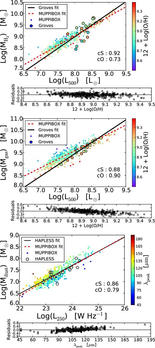
Correlation between IR luminosity and galaxy physical properties, for simulated galaxies and for galaxies from the Groves and HAPLESS samples. In the first two panels, data are colour-coded with gas metallicity, according to the colour bar on the right, while in the lower panel colour coding follows λpeak. Black continuous and red dashed lines give linear fits of the relations in the log–log plane, each panel reports the Spearman correlation coefficients for the simulation (cS) and for the observations (cO). Residuals of simulated galaxies are shown below each panel against gas metallicity (first two panels) and λpeak (bottom panel). Top panel: L500 luminosity against molecular mass |$M_{{\rm H}_2}$|. Middle panel: L500 against total gas mass |$M\rm {_{gas}}= M_{H{\rm \small {\,i}}} + M_{H_2}$|. In these two cases, data are from the Groves sample. Bottom panel: L250 against dust mass Mdust, data taken from the HAPLESS sample.
Conversely, correlation with total gas mass of MUPPIBOX galaxies shows systematic differences from the data; the tension is marginal, as the measured slopes are 0.75 ± 0.03 and 0.98 ± 0.18 for the simulated and observed samples, respectively. Galaxies in the Groves sample appear consistent with the lower envelope of the simulated relation. The figure shows a clear correlation of residuals of simulated galaxies with gas metallicity. Moreover, galaxies in the Groves sample appear to have systematically higher metallicities. We noticed from Fig. 2 that simulated galaxies tend to have higher gas metallicities and lower |${\rm H\,\small {i}}$| gas content than observed ones, and this is especially true for the small galaxies that dominate the sample in number. Groves galaxies have metallicities typically larger than |$12+{\rm {\rm l}og\,}({\rm O/H})\sim 8.9$|, that is, at +1σ of the Tremonti et al. (2004) relation. Therefore, the difference in metallicity cannot be due to the bias in metal content of simulated galaxies but is an observational bias, presumably due to the fact that low-metallicity galaxies tend to be CO-blind and so are not present in this sample. If we limit ourselves to galaxies in the same metallicity range >9.0, the slope changes to 0.78 ± 0.02 and the two slopes become consistent at 1σ.
Besides, our simulations predict that lower metallicity galaxies will be, at fixed total gas mass, less luminous at 500 μm, though this effect is less evident when molecular gas is used. In light of the results of Fig. 6, where gas and dust masses were found to correlate better with L500 than SFR, we conclude that this behaviour is due to the reprocessing of starlight by the diffuse component, whose dust content scales with metallicity.
The lower panel of Fig. 7 shows the correlation of L250 with dust mass. Data are taken from the HAPLESS sample, where dust masses were estimated from SED fitting. The simulated and observed data sets show very good agreement in the degree of correlation between the two quantities, the slopes being 0.63 ± 0.03 and 0.60 ± 0.19, respectively. Again, the agreement worsens when a dust emissivity index β = 1.6 is used. Clark et al. (2015) noticed that residuals on this relation correlate with the temperature of the cold dust component, obtained by fitting the SED with two modified black bodies of higher and lower temperature. grasil-3d computes dust temperatures in a self-consistent way, but obtains a whole range of values. We prefer to use the position of the ∼ 100 μm peak, λpeak, of the IR emission as a proxy of the average temperature of the cold dust component, larger values denoting lower temperatures. Simulated galaxies are thus colour-coded with λpeak. A clear dependence of residuals on the position of the peak is visible, with colder dust having lower 250 μm luminosity at fixed dust mass; this is the expected behaviour of a (modified) blackbody. Moreover, we did not find any significant dependence of residuals on gas metallicity.
4.4 On the position of the FIR peak
An issue addressed by Clark et al. (2015) is the source of heating of cold dust. The general idea is that the colder component of dust is prevalently heated by old stellar populations (e.g. Draine et al. 2007; Kennicutt et al. 2009), even though the exact geometry of the galaxy will influence the details. The results of Fig. 6 are also in line with the idea that colder components, dominating the longest wavelengths, are less well correlated with SFR, as if young stars were not any more the main source of energy. To verify this hypothesis, Clark et al. (2015) considered the correlation of cold gas temperature, obtained by fitting the SED with two modified black bodies for cold and warm dust, with proxies of light coming from young stars or from the bulk of stellar mass. For the first quantity they chose the ratio of SFR, measured from GALEX FUV and WISE 22 μm fluxes, and the estimated dust mass, while for the second quantity they chose the ratio between the Ks-band luminosity, a proxy of stellar mass and dust mass. They showed that the correlation of cold dust temperature with SFR/Mdust is higher than that with |$L_{K_{\rm s}}/M_{\rm dust}$|. We repeat their analysis, using again the position of the FIR peak, λpeak, as a proxy of cold dust temperature, and the quantities SFR/Mdust and M⋆/Mdust to mark the relative role of young and old stars. We recall again that SFRs are averaged over 100 Myr. Fig. 8 shows the resulting correlations. In this case, we do not report the HAPLESS data, because the quantities they use are inconsistent with ours. None the less, we recover their result: λpeak correlates well with the SFR per unit dust mass, while the correlation with the ratio of dust and stellar mass is visible only in galaxies with the highest M⋆/Mdust ratio. This is confirmed by the correlation coefficient reported in the panels. We conclude that in our simulated galaxies, while the role of SFR is less prominent in setting the temperature of the colder dust components and then the IR luminosity in the sub-mm range, young stars (with ages <100 Myr) are still the largest contributors to the radiation field responsible for dust heating (see also Silva et al. 1998).

Correlation of λpeak with SFR per unit dust mass (left-hand panel) and stellar mass per unit dust mass (right-hand panel). Points denote MUPPIBOX galaxies, colour coding is based on gas metallicity, as given by the colour bar. Each panel reports the correlation coefficient of the points.
5 SUMMARY AND CONCLUSIONS
We presented predictions of panchromatic SEDs of simulated galaxies at z = 0, obtained with a modified version of the TreePM-SPH code gadget3 that implements chemical evolution, metal cooling and the novel sub-resolution model MUPPI (Murante et al. 2015) for feedback and star formation, but contains no AGN feedback. Simulations were post-processed using the grasil-3d code (Domínguez-Tenreiro et al. 2014), a radiative transfer code that is based on grasil formalism (Silva et al. 1998; Silva 1999; Granato et al. 2000). In MUPPI, the molecular fraction of a gas particle is computed on the basis of its pressure, as in equation (1), based on the phenomenological relation of Blitz & Rosolowsky (2006). In grasil-3d stars younger than a time tesc are modelled as embedded in MCs with a given optical depth, while radiative transfer is computed taking into account the atomic gas, or cirrus component. The two codes share the rationale with which they divide the computation into resolved and sub-resolution elements. Post-processing by grasil-3d was then performed using the molecular fraction produced by the simulation. However, molecular gas was re-distributed around star particles younger than tesc, produced by a stochastic star formation algorithm, to ensure the coincidence of the two components in a way that is consistent with model assumptions.
In this paper, we addressed the Universe at z = 0, where high-quality data are available. We first checked that the 498 galaxies produced by our code in a cosmological volume of 25 Mpc (H0 = 72 km s−1 Mpc−1) present properties such as stellar masses, SFRs (averaged over 100 Myr), gas metallicities, atomic and molecular gas masses, dust masses, B/T ratios in broadly agreement with observations. Consistently with other simulation projects (e.g. Genel et al. 2014; Vogelsberger et al. 2014; Lagos et al. 2015; Schaye et al. 2015; Bahé et al. 2016), galaxy properties are realistic, though at tension with observations both at masses below 1010 M⊙, where galaxies are more passive, metallic and less gas rich than observed ones (a well-known problem of galaxy formation in ΛCDM; Fontanot et al. 2009b; Weinmann et al. 2012), and at masses above 1011 M⊙, where the lack of AGN feedback produces blue massive galaxies.
Our main results are the following:
The SEDs of simulated galaxies resemble the observed ones, from FUV to sub-mm wavelengths. We checked this by comparing average SEDs, in bins of stellar mass or SFR, with data from LVL (Cook et al. 2014b,a), PEP (Gruppioni et al. 2013) and HRS Boselli et al. (2010); Ciesla et al. (2014) samples. The comparison with LVL and PEP, which are subjected to different selection biases, was performed by normalizing SEDs to the same 3.6 μm flux, while the comparison with HRS was done considering also the normalization. SED comparison confirms that the escape time of stars from their MCs should be relatively short, tesc = 3 Myr. Simulated and observed SEDs show some disagreement only for the smallest galaxies, where tension with observations is higher and their variation of shape follow the same trends with stellar mass and SFR. An excess of attenuation in the FUV is interpreted as the result of excessive gas metallicities in simulated galaxies.
We quantified, using the Spearman coefficient, the correlation of IR luminosities in Spitzer and Herschel bands, from 3.6 to 500 μm, with stellar mass, SFR, molecular gas mass, atomic gas mass and dust mass. The correlation with stellar mass drops for λ > 5 μm, and SFR is the quantity that best correlates with IR luminosity up to 160 μm, while at longer wavelengths tighter correlations are shown by molecular gas and, eventually, dust masses. This is a sign that the cold dust components receive non-negligible contributions by old stars. The best correlation of IR luminosity with SFR is found at 8 μm, while at 24 μm PAH emission causes a decrease of the correlation coefficient. Dust and atomic gas masses show the worst correlations, though dust mass overtakes SFR at 500 μm.
We used Groves and HAPLESS samples to further investigate the correlation of IR luminosity and gas or dust masses. We found very good agreement with data, with the exception of atomic masses. However, we found the difference to be due to a bias of Groves galaxy in favour of high-metallicity ones. This shows that, despite the mild tension with observations, simulated samples can be used to understand the physical and selection properties of observed galaxy samples.
We confirm the findings of Clark et al. (2015) that the scatter in the relation between L250 and Mdust is due to varying temperature of cold dust, using the position of the IR peak λpeak as a proxy for the temperature of cold dust. We further showed that λpeak is determined by SFR more than stellar mass. Together with the correlation trends discussed above, this implies that although the colder dust components that dominate sub-mm emission are heated non-exclusively by young stars (<100 Myr), their contribution remains the most prominent one. This is partially in contrast with the canonical picture in which cold dust is heated by evolved stellar populations (e.g. Draine et al. 2007; Kennicutt et al. 2009).
These results demonstrate the ability of our hydrodynamical simulation code to produce galaxies that, at z = 0, resemble the observed galaxies in our local Universe not only in their physical, structural parameters but also in their observational manifestations. The point in common between our hydro code and the grasil-3D radiative transfer solver is a description of physics at sub-kpc scales through sub-grid models, MUPPI on the hydro side and the treatment of MCs and dust on the grasil-3D side. Our tests show that this combination works well: tensions of simulated galaxy SEDs with respect to observations can be understood as the result of tensions in their structural parameters, while a good degree of predictivity is shown in our detailed comparison of simulations and data of local galaxies. This work can be seen as a validation test to use these simulations as a tool to gain insight into observed galaxies and to extend the predictions to high redshift. This will allow on the one hand to better constrain simulation results by performing comparisons in terms of observables, instead of physical quantities, like stellar masses or SFRs, recovered through techniques that require a number of assumptions that should better be done on the theory side. On the other hand, it will allow us to forecast the results of future surveys and to understand at a deeper level which observables are best suited for constraining the history of galaxies.
Acknowledgments
We thank D. Cook, C. Gruppioni and X.-J. Jiang for providing their data, and Volker Springel who provided us with the non-public version of the gadget3 code. We acknowledge useful discussions with L. Silva, D. Calzetti, Raffaella Schneider, F. Fontanot, P. Barai, G. De Lucia, C. Mongardi and A. Zoldan.
This work is supported by the PRIN-INAF 2012 grant ‘The Universe in a Box: Multi-scale Simulations of Cosmic Structures'. The simulations were carried out at the ‘Centro Interuniversitario del Nord-Est per il Calcolo Elettronico' (CINECA, Bologna), with CPU time assigned under University-of-Trieste/CINECA and ISCRA grants; the analysis was performed on the facility PICO at CINECA under the ISCRA grant IscrC_GALPP.
We thank the MICINN and MINECO (Spain) for grants AYA2009-12792-C03-03 and AYA2012-31101 from the PNAyA. AO was financially supported through a FPI contract from MINECO (Spain).
Parts of this research were conducted by the Australian Research Council Centre of Excellence for All-sky Astrophysics (CAASTRO), through project number CE110001020. This work was supported by the Flagship Allocation Scheme of the NCI National Facility at the ANU.
This research has made use of ipython2 (Perez & Granger 2007), scipy3 (Jones et al. 2001), numpy4 (van der Walt, Colbert & Varoquaux 2011) and matplotlib5 (Hunter 2007).
REFERENCES
APPENDIX A: TESTS ON grasil-3d
This appendix is devoted to study in more detail the effects on the galaxy SED of (i) the grid size adopted by grasil-3d to perform the radiative transfer calculation, (ii) the aperture size to identify galaxies and (iii) the impact of the dust emissivity index on the FIR emission.
To perform these tests we use two galaxies, a normal one (ID12318) and a recent merger (ID3); both stellar masses are close to the median value of MUPPIBOX sample. We also use the massive late-type galaxy (GA1), extracted from a zoom-in simulation and fully described in Murante et al. (2015) and Goz et al. (2015) (their lower resolution case); its mass resolution and force softening are comparable to those of MUPPIBOX. In Table A1, we list the main characteristics of the three selected galaxies. All the quantities marked by (Rgal) are evaluated within the galaxy radius, taken as 1/10 of the virial radius of the host halo, while by (RP) within the Petrosian radius defined in Section A2. Gas mass includes, as in the main text, multiphase gas particles and single-phase ones with temperature lower than 105 K.
Basic characteristics of selected galaxies. Column 1: simulation name; Column 2: galaxy radius (kpc), set to 1/10 of the virial radius; Column 3: Petrosian radius (kpc), defined in equation (A2); Column 4: B/T ratio inside the galaxy radius; Column 5: B/T ratio inside the Petrosian radius; Column 6: total galaxy stellar mass (M⊙), inside the galaxy radius; Column 7: total galaxy stellar mass (M⊙), inside the Petrosian radius; Column 8: total galaxy gas mass (M⊙), inside the galaxy radius; Column 9: total galaxy gas mass (M⊙), inside the Petrosian radius; Column 10: total galaxy dust mass (M⊙), evaluated by grasil-3d, inside the galaxy radius; Column 11: total galaxy dust mass (M⊙), evaluated by grasil-3d, inside the Petrosian radius.
| Galaxy | R(gal) | R(P) | B/T|${_{(R_{\rm gal})}}$| | B/T|${_{(R_{\rm P})}}$| | M|$_{\star {(R_{\rm gal})}}$| | M|$_{\star {(R_{\rm P})}}$| | |$M{}{_{{\rm {gas}} (R_{{\rm gal}})}}$| | M|${_{{\rm {gas}} (R_{\rm P})}}$| | M|${_{{\rm {dust}} (R_{\rm gal})}}$| | M|${_{{\rm {dust}} (R_{\rm P})}}$| |
|---|---|---|---|---|---|---|---|---|---|---|
| GA1 | 30.37 | 12.41 | 0.22 | 0.23 | 1.35 × 10¹¹ | 1.15 × 10¹¹ | 2.44 × 10¹¹ | 1.84 × 10¹⁰ | 2.69 × 10⁸ | 1.89 × 10⁸ |
| ID12318 | 9.39 | 6.52 | 0.49 | 0.53 | 4.31 × 10⁹ | 3.76 × 10⁹ | 1.65 × 10⁹ | 1.14 × 10⁹ | 1.48 × 10⁷ | 1.03 × 10⁷ |
| ID3 | 17 | 4.43 | 0.34 | 0.59 | 5.1 × 10⁹ | 1.85 × 10⁹ | 2.45 × 10⁹ | 7.12 × 10⁸ | 2.01 × 10⁷ | 4.95 × 10⁶ |
A1 Stability with grid size
Force softening sets the space resolution of the simulation. grasil-3d uses a Cartesian grid to compute the density of star and gas components, whose size is clearly set by softening to within a factor of order unity.

The variation on the SED, defined as in equation (A1), in function of the wavelength for the GA1 galaxy. The grid size is set to two times (red line) and four times (blue dashed line) the force softening of the simulation.
On ID12318 galaxy and ID3 merger, we found that the SED is mostly unaffected when using grids of one or two softening lengths, with the exception of variations of at most 10 per cent in the PAH region. On the contrary, grid sizes of four times the force softening, showed significant variations of the SED up to ≃ 20 per cent in the FUV, ≃ 50 in the PAH region and ∼30 per cent at the FIR peak. We extended this test to the average SED of the whole MUPPIBOX sample, showing negligible variations when the grid is set to one or two softening lengths.
We concluded that results are very stable as long as the grid size is ≤2 softening lengths. Computational times are very sensitive to the value of the grid, so we used the softening length to compute SEDs for our main results, but used two softening lengths to perform the robustness test of grasil-3d parameters (Section 4.2).
A2 Choice of galaxy aperture
We post-processed using grasil-3d these galaxies selecting their galaxy particles within RP. We then checked how galaxy SEDs change when the galaxy particles are selected within Rgal = 0.1Rvir or RP. The Petrosian aperture translates in a lower luminosity at all wavelengths, so its effect is quantified by the change in stellar and gas masses. More massive galaxies, M⋆ ≳ 1011 M⊙ tend to have extended stellar haloes, so their luminosities have a more marked dependence on aperture (this is found in observed galaxies as well, as shown for instance by Bernardi et al. 2013). In fact, the stellar mass of GA1 decreases by 17 per cent from Rgal to RP, while the lower mass galaxy ID12318 changes by 14 per cent. For the peculiar ID3 object, the Petrosian aperture leads to the exclusion of the merger and the stellar mass of the resulting object decreases by nearly a factor of 3.
A3 Modified blackbody emission
where Bλ(Tdust) is a blackbody at temperature Tdust and β is the dust emissivity index. This approach is based on laboratory experiments; these however show temperature-dependent spectral slope variations (Boudet et al. 2005). The most recent results also show that the emissivity index varies with wavelengths (Coupeaud et al. 2011) and suggest 1.5 < β < 2.5 (see discussion in Jones 2014). grasil-3d employs the canonical approach by Draine & Lee (1984), which yields a power-law decline β = 2, while recent Planck observations of MW dust in the diffuse ISM (Planck Collaboration XVI 2014) indicate a dust emissivity index β = 1.62 ± 0.10. We tested on the GA1 galaxy that, adopting the lowest value β = 1.6, the SED is basically unaffected below the peak at λpeak ≃ 100 μm, while above the luminosity is enhanced by about 60 per cent at ≃500 μm. The SEDs of ID12318 and ID3 galaxies were much less affected by this change. As we mentioned in the main text, the correlations of IR luminosity with H2 and dust masses show a worse agreement with data when β = 1.6 is used.
APPENDIX B: DEPENDENCE OF SEDS ON grasil-3d PARAMETERS
We divide LVL, PEP and our MUPPIBOX samples in different stellar mass bins (columns in Fig. B1), and for each of them we post-process with grasil-3d the simulated galaxies, at fixed |$M\rm _{MC}$| (rows in Fig. B1), employing different values for |$t\rm _{esc}$|. We used grid values equal to twice the softening for this test (see Appendix A1) in order to save computational time. In these plots, masses are in M⊙, |$t\rm _{esc}$| in Myr and the resulting SEDs are normalized to the IRAC1 band (3.6 μm). In every plot, orange and violet dot–dashed lines represent the median value for PEP and LVL samples, respectively, while the corresponding filled regions show the 1σ uncertainty obtained using the 16th and 84th percentiles and, finally, the continuous colour lines show the median values of MUPPIBOX galaxies for different escape times |$t\rm _{esc}$|.

Dependence of SEDs on grasil-3d parameters. In the column on the left, the galaxies are selected in the mass range of 9.3 < log (M⋆) < 9.5 M⊙, on the middle in the mass range of 9.5 < log (M⋆) < 10 M⊙ and on the right in the mass range of 10 < log (M⋆) < 10.5 M⊙, for MMC = 105 M⊙ (top row), MMC = 106 M⊙ (middle row) and MMC = 107 M⊙ (bottom row). In each plot, all the SEDs are normalized to the IRAC1 band (3.6 μm), continuous colour lines show the median values for different tesc, while orange and violet dot–dashed lines represent the median value for PEP and LVL samples, respectively, and finally the corresponding filled regions give the 1σ uncertainty. Every plot reports the number of galaxies in the MUPPIBOX, PEP and LVL samples.
We explore reasonable ranges for tesc (2, 3, 4, 5 Myr), and MMC (105–106–107 M⊙), as adopted in previous works (e.g. Silva et al. 1998; Granato et al. 2000; Domínguez-Tenreiro et al. 2014; Obreja et al. 2014; Granato et al. 2015). As expected, with tesc increasing from 2 to 5 Myr at fixed |$M\rm _{MC}$|, the UV emission decreases, but the MC cloud emission increases and, at the same time, the cirrus emission in the PAH region decreases. Hence, the net result is that the emission increases from the PAH region up to ∼100 μm, leaving the peak unaffected. On the other hand, as |$M\rm _{MC}$| increases from 105 up to 107 M⊙ at fixed tesc, the cirrus emission is unaffected, but the bulk of the MC emission moves to longer wavelengths (lower dust temperature) due to the increased optical depth. The net result is a decreased emission in the PAH region but a higher IR peak.
Now we discuss the results for every mass bin, represented by the columns in Fig. B1.
Left column – 9.3 < log (M⋆) < 9.5 M⊙:
From FUV up to mid-IR (∼10 μm) there is not substantial variation among different values of |$M\rm _{MC}$| which, on the contrary, mostly affect the IR peak. The PAH emission is considerably enhanced by the highest value tesc = 5 Myr, even if for |$M\rm _{MC}$| = 107 M⊙ the bulk of the MC emission is considerably shifted at lower frequency due to the increased optical depth, depleting for all the available tesc the PAH emission.
Middle column – 9.5 < log (M⋆) < 10 M⊙:
The global trend reflects what has been already discussed for the previous mass bin. The SEDs with values tesc = 3–4 Myr are quite well in agreement with PEP and LVL samples in the PAH region, except for the highest value |$M\rm _{MC}$| = 107 M⊙.
Right column – 10 < log (M⋆) < 10.5 M⊙:
The SEDs with lower values tesc = 2–3 Myr are better in agreement with PEP and LVL samples in the PAH region.
In all the explored mass bins, the highest |$M\rm _{MC}$| = 107 M⊙ appears to overestimate the optical depth enhancing the IR-emission and at the same time to decrease the PAH emission. |$M\rm _{MC}$| = 106 M⊙ fits better in all the mass bins the PEP and LVL's median values. Furthermore, the best values for the escape time are low-intermediate ones, i.e. tesc = 2–3 Myr.
In Fig. B2, we show the results for all the galaxies (log M⋆ > 9.3 M⊙). tesc = 3 Myr fits better the median PEP and LVL's values in the PAH region. There is not substantial difference between 105 and 106 M⊙ for the |$M\rm _{MC}$|.

Dependence of SEDs on grasil-3d parameters. In all plots, only galaxies with log (M⋆) > 9.3 M⊙ and |$M\rm _{MC}$| = 105 M⊙ (left), |$M\rm _{MC}$| = 106 M⊙ (middle), |$M\rm _{MC}$| = 107 M⊙ (right) are taken into account. In each plot, all the SEDs are normalized to the IRAC1 band (3.6 μm), continuous colour lines show the median values for different tesc, while orange and violet dot–dashed lines represent the median value for PEP and LVL samples, respectively, and finally the corresponding filled regions give the 1σ uncertainty. Every plot reports the number of galaxies in the MUPPIBOX, PEP and LVL samples.
This test shows that the dependence of SEDs on the value of MMC is modest, while tesc influences the FUV bands and, especially, the MIR region dominated by the PAH lines, down to ∼ 30 μm. The values adopted in the paper of tesc = 3 Myr is a very good compromise value.
