


Abstract
In the next decade, new astrophysical instruments will deliver the first large-scale maps of gravitational waves (GWs) and radio sources. Therefore, it is timely to investigate the possibility to combine them to provide new and complementary ways to study the Universe. Using simulated catalogues appropriate to the planned surveys, it is possible to predict measurements of the cross-correlation between radio sources and GW maps and the effects of a stochastic GW background on galaxy maps. Effects of GWs on the large-scale structure (LSS) of the Universe can be used to investigate the nature of the progenitors of merging black holes, the validity of Einstein's general relativity, models for dark energy and detect a stochastic background of GW. The results obtained show that the galaxy–GW cross-correlation can provide useful information in the near future, while the detection of tensor perturbation effects on the LSS will require instruments with capabilities beyond the currently planned next generation of radio arrays. Nevertheless, any information from the combination of galaxy surveys with the GW maps will help provide additional information for the newly born GW astronomy.
1 INTRODUCTION
The detection by the Laser Interferometer Gravitational-Wave Observatory (LIGO) instrument of gravitational waves (GWs; GW150914, Abbott et al. 2016a and GW151226, Abbott et al. 2016d) from the merger of binary black holes (BBHs) opened up a new window to study our Universe. In the first few months following the first detection, GWs have been used to test general relativity in a new way (Abbott et al. 2016c), the speed of GWs (Bettoni et al. 2017; Blas et al. 2016; Collett & Bacon 2017; Kahya & Desai 2016) and alternative cosmological models such as the one where the dark matter is made of primordial black holes (e.g. Bird et al. 2016).
Currently and for the foreseeable future, the main way to detect GWs is by the use of laser interferometers, on Earth and in space. Several alternatives have been proposed, and they involve detecting the effect of GWs on other observables, such as Pulsar timing arrays (Lorimer & Kramer 2005), the effect of GWs from inflation on the cosmic microwave background (CMB; Kamionkowski & Kovetz 2016), and the effect of GWs on the large-scale structure (LSS) of the Universe (Guzzetti et al. 2016).
The presence of tensor modes during the early epochs of the Universe modifies the power spectrum of primordial scalar perturbations (Jeong & Kamionkowski 2012), while at late times the presence of a GW background leads to several effects, including projection effects due to the perturbation of space–time by GWs on the galaxy distribution (Jeong & Schmidt 2012; Schmidt & Jeong 2012a), the CMB (Dodelson, Rozo & Stebbins 2003; Cooray, Kamionkowski & Caldwell 2005; Book, Kamionkowski & Souradeep 2012a) and the 21-cm background (Pen 2004; Book, Kamionkowski & Schmidt 2012b).
At the same time, radio surveys for cosmology are entering a new phase of exponential expansion on both quantity and quality of data available (Norris et al. 2013), with the construction of several instruments, including the Australian Square Kilometre Array Pathfinder (ASKAP; Johnston et al. 2008) and the design definition of the Square Kilometre Array (SKA1). Radio galaxy surveys with such instruments will be able to detect galaxies over a large redshift range, a wide area of the sky, and down to a very low flux limit.
Radio surveys such as NVSS have been used in the past to perform cosmological analyses (see e.g. Nolta et al. 2004; Raccanelli et al. 2008; Xia et al. 2010; Bertacca et al. 2011); future surveys will have a wider redshift range and orders of magnitude and more objects observed, so it is expected they will improve the precision of cosmological measurements (Raccanelli et al. 2012). All this, combined with the fact that effects of GWs on LSS are largest at very large scales, makes it very timely to start an investigation of the combination of GW with radio galaxy maps.
This paper investigates the possibility to use future radio galaxy surveys to contribute to GW astronomy. By measuring the position and correlation of galaxies, or cross-correlating their number counts with GW maps, it will be possible to detect direct or indirect effects of GWs coming from the merger of massive compact objects or the early stages of the Universe.
GW astronomy is still in its infancy but it is predicted to grow quickly, and the coincidental exponential increase in radio survey capabilities makes it very interesting to analyse how to best combine the two fields. Therefore, it is timely to try to understand if the combination of observations of radio sources and GWs can give useful additional information about cosmological models and parameters currently investigated.
We will present forecasts of the constraints on cosmological models and parameters that will be possible to obtain both by cross-correlating future GW maps with galaxy catalogues from a variety of planned radio surveys, and by analysing the effect of GWs on position, distribution and correlation of such galaxy catalogues. Recently, ideas about cross-correlation of LSS with GW maps have been explored in e.g. Camera & Nishizawa (2013), Oguri (2016), Namikawa, Nishizawa & Taruya (2016a), Raccanelli et al. (2016c).
The structure of the paper is as follows. In Section 2, we introduce the radio galaxy surveys we consider. In Section 3, we present the studies that will be enabled by cross-correlating GW with galaxy maps, in particular angular correlations to determine the progenitor of BBH mergers in Section 3.1 and constraints on cosmic acceleration models by using lensing effects on radial correlations in Section 3.2. In Section 4, we investigate the effects of GWs on the LSS; we predict measurements that will be possible to obtain by using cosmometry in Section 4.1 and the cosmic rulers methodology in Section 4.2. We then summarize our findings and conclude in Section 5.
2 FORTHCOMING RADIO GALAXY SURVEYS
In this paper, we focus on forthcoming radio galaxy surveys; we consider the Square Kilometre Array (SKA; Maartens et al. 2015) and its pathfinders (Norris et al. 2013), in particular the cosmology survey Evolutionary Map of the Universe (EMU; Norris et al. 2011) with the ASKAP instrument. We will consider both radio continuum and H i spectroscopic cases.
We model radio surveys by using the prescription of Wilman et al. (2008); catalogues are generated from the S-cubed simulation,2 using the SEX and SAX for continuum and H i surveys, respectively. We then apply a cut to the simulated data to reflect the assumed flux limit for different cases. More details on the underlying modelling and planned surveys can be found in Wilman et al. (2008); Jarvis et al. (2015); Abdalla et al. (2015). Finally, for all surveys we assume fsky = 0.75. We expect that for some measurements, in particular the detection of GW effects using only radio surveys, the area, redshift range and number density required will often be surpassing the specifications of planned instruments. Therefore, we include in our predictions instruments with futuristic capabilities, which will be used to understand if those measurements will be possible even in principle.
Although radio continuum surveys do not have in principle redshift information, there are a variety of techniques that could enable the possibility to divide the galaxy catalogue into redshift bins. A detailed comparison of methodologies is beyond the scope of this paper, where we assume the clustering-based redshift (CBR) information proposed in Ménard et al. (2013). We will assume the possibility to divide the catalogue into bins using the CBR technique following Kovetz, Raccanelli & Rahman (2017).
2.1 EMU
At its completion, ASKAP will consist of 36 12-m antennas spread over a region 6 km in diameter. EMU is an all-sky radio continuum survey that will cover the whole southern sky, extending as far north as +30°, with a sensitivity of 10 μJy beam−1 rms, over a frequency range of 1130–1430 MHz. It will be a particularly fast survey, thanks to the phased-array feed (PAF) at the focus of each antenna, which gives ASKAP a 30 deg2 of instantaneous field of view. It is expected to detect ∼70 million galaxies, which will make it the largest radio galaxy survey so far.
2.2 SKA
The SKA is an international multipurpose next-generation radio interferometer that will be built in phases (SKA1 and SKA2) in the Southern hemisphere in South Africa and Australia; it will cover a frequency range of 350 MHz–15 GHz, have a central core of ∼200 km diameter, with three spiral arms spreading over 3000 km and a total collecting area of about 1 km2. SKA is a facility that is planned to last for around 50 yr, and it will continuously scan the sky, producing a vast amount of data. Among many types of observations delivered by such instruments, we focus here on surveys that will detect individual galaxies, neglecting e.g. intensity mapping surveys. On longer time-scales, one can envisage significant improvements with respect to the instruments planned at the moment.
2.2.1 Radio continuum
Being unaffected by dust, radio continuum emissions can be used to detect SFGs and AGN up to very high redshift. Radio continuum surveys with the SKA will observe 30 000 deg2 out to extremely high redshift, detecting ∼108 galaxies in SKA1 and ∼109 in SKA2.
In the top panel of Fig. 1, we show the predicted redshift distributions for continuum surveys. We show three different flux limits Slim: (i) 50 μJy, corresponding to a 5σ detection for sources with the planned full EMU survey; (ii) an SKA-like 1μJy limit, and (iii) a futuristic distribution including all sources down to 1 nJy. In the legend, we also include the total number of objects per square degree, that corresponds to ≈8500, 135 000, 550 000, respectively.

Number of sources per deg2, as a function of redshift, for different flux limits. Top panel: radio continuum surveys; bottom panel: H i galaxy surveys. In the legend is the total number of objects. Distributions taken from the S3 simulation.
2.2.2 H i
While current H i galaxy surveys are not competitive with wide optical ones, technological advancements that will be implemented in the SKA will allow for dramatically faster survey speeds, making it possible to map the galaxy distribution out to high redshifts over large areas, therefore enabling measurements of ultra-large scales. Once the full SKA2 will be in place, it will provide what has been called the ‘billion galaxy survey’, that will be the biggest spectroscopic galaxy survey to date, detecting ∼109 galaxies over 30 000 deg2 out to z ∼ 2.
In the lower panel of Fig. 1, we plot the predicted redshift distributions for H i surveys. Again, we show three different cuts in sensitivity: (i) 5 μJy, corresponding roughly to the planned sensitivity of the SKA2 galaxy survey, (ii) a more optimistic 1 μJy, and once again (iii) a futuristic distribution including sources down to 1 nJy.
In order to keep our results as general as possible, we define surveys in terms of full sky surveys with the above flux limits. The two cases of Slim = 1 nJy are shown as a proof of principle of what very futuristic surveys could in principle achieve. In addition, in order to investigate what can be done in the future (and possibly helping the planning of future instruments), we will in some cases study what instrument specifications would allow specific measurements.
2.2.3 Bias
The S3 simulation provides us with a source catalogue where sources are identified by type; each of these has a different prescription for the bias, as described in Wilman et al. (2008). We use the models of Raccanelli et al. 2012 (for continuum surveys) and of Santos et al. 2015 (for H i surveys) to assign the bias to sources at different flux limits. In Fig. 2, we show an example of the bias used for continuum and H i galaxy surveys with a flux limit of 10 μJy.
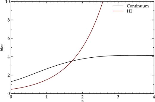
Bias for the radio continuum (black) and H i (red) galaxy surveys for an example flux limit of 10 μJy.
3 GALAXY–GW CROSS-CORRELATIONS
One of the most used observables in the analysis of galaxy surveys is the galaxy power spectrum (or correlation functions). It is possible to extract a trove of information from radial and angular correlations (see e.g. Raccanelli et al. 2013, 2015b, 2016d), both by auto-correlating galaxies and by cross-correlating galaxies from different galaxy surveys (see e.g. Bacon et al. 2015) or with other observables, such as CMB temperature maps (see e.g. Bertacca et al. 2011; Raccanelli et al. 2015a). A summary of cosmological measurements from auto- and cross-correlations using radio continuum surveys can be found in Raccanelli et al. (2012).
In this section, we focus on cross-correlations of radio galaxy with GW maps, both by correlating samples in the same redshift range to investigate properties of BBH mergers, and by looking at radial cross-correlations in different redshift bins, in order to detect the lensing of GWs by foreground galaxies, and use this measurement to constrain models that explain the cosmic acceleration.
In Section 3.1, we briefly summarize the methodology for determining the nature of BBH progenitors, presented in Raccanelli et al. (2016c), and present updated forecasts.
Radial cross-correlations can be used to test models of dark energy and modified gravity, as first suggested by Cutler & Holz (2009) and then further studied in Camera & Nishizawa (2013); in Section 3.2, we will analyse this technique in the context of radio surveys correlated with BBH mergers.
3.1 Angular cross-correlations
The angular cross-correlation of galaxy catalogues with the GW maps is a natural way to investigate properties of the progenitors of compact objects whose mergers give rise to the GWs detected by laser interferometers, such as the hypothesis that BBH trace matter inhomogeneities (Namikawa et al. 2016a), or to constrain the distance–redshift relation (Oguri 2016).
In a similar way, Raccanelli et al. (2016c) recently suggested that the cross-correlation of star-forming galaxies (SFG) with GW maps can constrain the cosmological scenario in which the dark matter is comprised of primordial black holes (PBHs).
PBHs were first studied in Zel'dovich & Novikov (1967); Hawking (1971); Carr & Hawking (1974), and a vast literature on the topic was then produced. The possibility that they could make up the dark matter was first investigated in Garcia-Bellido, Linde & Wands (1996); Nakamura et al. (1997). However, these models were predicting PBHs of relatively small masses (∼1 M⊙), that were subsequently ruled out by microlensing experiments (Wyrzykowski et al. 2011).
Recently, the LIGO detection of the merger of BBHs of larger masses (∼20–30 M⊙) suggested that these objects might be quite common. Interestingly enough, the combination of observational constraints from microlensing and disruption of wide binaries (Wyrzykowski et al. 2011; Monroy-Rodríguez & Allen 2014) rule out the possibility of PBHs as DM for BHs with masses below ∼10 M⊙ and above ∼80 M⊙, but leave open the window in between.3
Therefore, Bird et al. (2016) suggested that PBHs of 30 M⊙ comprise the dark matter; other suggestions including models with a wider mass distribution have been then studied in Clesse & García-Bellido (2017); Sasaki et al. (2016); for a recent more general review on PBHs as DM, see Carr, Kuhnel & Sandstad (2016). In addition, calculations of the formation of binary systems of such objects and their merger rate overlaps with estimates based on the first aLIGO observations. Given the ongoing difficulty in detecting weakly interacting massive particles, this model recently attracted a lot of attention and it is therefore important to develop methods to test it, and more generally determine the nature of BBH progenitors.
In this work, we follow the same formalism of Raccanelli et al. (2016c), but using an updated (including the most recent LIGO data) merger rate of 1–10 Gpc−3 yr−1, and a wider redshift range, with |$z_{\rm max}^{\rm H\,{\small i}}=3$| and |$z_{\rm max}^{\rm cont}=5$|, for H i and continuum radio surveys, respectively.
A key element to determine the nature of the progenitors of BH–BH mergers is represented by the value of the halo bias of the mergers’ hosts. While we expect that mergers of objects at the endpoint of stellar evolution will be hosted by galaxies that contain the majority of stars, and therefore be hosted in haloes of ∼1011 − 12 M⊙, almost all mergers of PBH binaries would happen in haloes of <106 M⊙, as shown in Bird et al. (2016). Crucially, these two types of haloes will have very different values of the bias. In particular, we assume that galaxies that host stellar GW binaries have similar properties of the SFG galaxy sample. Hence, we assume that |$b^{\rm Stellar}_{GW} = b_{\rm SFG}$|, taking its redshift dependence as in Ferramacho et al. (2014). On the other hand, the bias of the small haloes that host most of the PBH mergers is expected to be ≲0.5, roughly constant with redshift, within our considered range (Mo & White 1996). Hence, considering that the bias of SFGs is predicted to be b(z) > 1.4, we set, for the threshold granting a detection, Δb = bSFG − bGW ≳ 1; this value should in reality increase with redshift, making our choice conservative.
It is worth noting that this scenario can be also tested by using the eccentricity of the binaries’ orbits before merging (Cholis et al. 2016); other ways to constrain properties of BBH mergers can be found in e.g. Kushnir et al. (2016), Stone, Metzger & Haiman (2017).
To predict the precision with which one can test models for the nature of the BBH progenitors, we consider the effective correlation amplitude, Ac ≡ r × bGW, where r is the cross-correlation coefficient of equation (2). The cross-correlation coefficient r parametrizes the extent to which two biased tracers of the matter field are correlated (Tegmark & Peebles 1998). This factor accounts for the fact that the two sources are not necessarily correlated, and its value ranges from 0 (totally uncorrelated) to 1 (perfectly correlated). In this context, an example could be the following: if sources of GW are astrophysical, for example coming from globular clusters, they would be originated in SFGs. However, if for any dynamical process they are ejected out of their host galaxy, then the correlation coefficient would be equal to the fraction of remaining merging binaries. This effect is not important unless very high angular resolution is achievable. However, given that this number is also completely degenerate with the other amplitudes, we will constrain the combined quantity Ac defined above.
Given that an important source of uncertainty is given by the galaxy bias, we compute a 2 × 2 Fisher matrix for the parameters {Ac, bg}, using a prior on the galaxy bias corresponding to a precision of 1 per cent in its measurement; measurements of the bias can be obtained either by fitting the amplitude of the auto-correlation of galaxy bias, or by other probes such as measurements of the bispectrum (Gil-Marín et al. 2015) or the cross-correlation with CMB-lensing (see e.g. Vallinotto 2012). Moreover, we assume the bias to be scale-independent and limit our analysis to linear scales.
We consider four different configurations of GW detectors, all assumed to observe the full sky. Raccanelli et al. (2016c) showed that the minimum angular scale to which the GW events can be localized plays an important role in improving the constraints on the galaxy–GW cross-correlation, as does the maximum redshift observable. An accurate determination of the value of ℓmax(=180°/θ) for all experiments and events is beyond the scope of this paper. Therefore, based on e.g. Finn (2010), Namikawa, Nishizawa & Taruya (2016b), we choose the specifications as shown in Table 1.
Specifications of GW detectors used in this paper. For cross-correlations with the Einstein Telescope, we use zmax = 2 for H i and zmax = 5 for continuum radio surveys.
| Experiment | ℓmax | zmax |
|---|---|---|
| aLIGO + VIRGO | 20 | 0.75 |
| LIGO-net | 50 | 1.0 |
| Einstein Telescope | 100 | 5 (2) |
| Einstein Telescope binned | 100 | 5 (2) |
| Experiment | ℓmax | zmax |
|---|---|---|
| aLIGO + VIRGO | 20 | 0.75 |
| LIGO-net | 50 | 1.0 |
| Einstein Telescope | 100 | 5 (2) |
| Einstein Telescope binned | 100 | 5 (2) |
When correlating GW maps from the Einstein Telescope (ET), we use zmax = 2 for H i surveys and zmax = 5 for continuum surveys; for the continuum case, we assume we can bin sources into bins of width Δz = 1, at the price of discarding 90 per cent of the sources (see Kovetz et al. 2016 for details). Considering the difficulty in determining a very precise redshift of GW events at high redshift, we take the safe assumption of having bins of Δz = 1 also for the H i case.
In Fig. 3, we show our predicted constraints. We show forecasts for the different GW interferometers setups, after 5 yr of collecting data, correlated with radio surveys. Vertical bars show the constraints when varying the merger rate |$\mathcal {R}\in [1,10]$|. Horizontal lines show the required precision in measurements of Ac to test the cases where the fraction of DM made of PBHs, fPBH, is <1. In the cases of aLIGO and the expanded LIGO-net, correlating with continuum or H i surveys will not make a difference. When using ET data, on the other hand, the maximum redshift used for galaxy surveys will make a difference, thus we show separate results for the correlations GW-radio galaxy for H i and continuum.
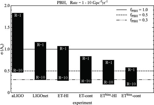
Forecast errors on the cross-correlation amplitude, Ac, for different fiducial experiment sets and varying merger rates. Each column corresponds to a GW detector experiment, for merger rates from 1 to 10 Gpc−3yr−1. The horizontal lines show the expected difference in the cross-correlation between primordial and stellar binary progenitors, for three different values of the percentage of DM made of PBHs.
As one can see, already in the case of aLIGO, if the merger rate will be towards the largest limits currently allowed by observations, one should be able to detect the signature of PBHs as DM within a few years. In the more futuristic cases of correlations of ET maps with binned continuum radio surveys, we can expect to have a few σ detection in the case of fPBH = 1, or detect the effects of a small fraction of DM consisting of PBHs.
3.2 Cosmic magnification
Gravitational lensing causes light rays to be deflected by large-scale structures along the line of sight, introducing distortions in the observed images of distant sources (Turner, Ostriker & Gott 1984). Even though surface brightness is conserved, the sources behind a lens are magnified in size, hence inducing an increase in the total observed luminosity of a source. Therefore, sources that are just below the flux threshold of a given survey will be magnified and become detectable, and so the observed number density of sources is increased. On the other hand, lensing causes the stretching of the observed field of view, leading to a dilution of the number density. The net result of these two competing effects depends on the slope of the source number count as a function of the sources luminosity, and the effect is called magnification bias. Observationally, we can detect the effects of magnification by cross-correlating two galaxy surveys with disjoint redshift distributions, as the observed number counts can be modified as explained above, and the intrinsic galaxy clustering is negligible for long radial correlations. The implications of this effect for the observed galaxy angular correlation function were investigated in e.g. Villumsen, Freudling & da Costa (1997), Kaiser (1998). Cosmic magnification has been suggested as a probe for cosmology by Matsubara (2000) and has been subsequently studied in a variety of works (see e.g. Hui, Gaztañaga & Loverde 2007; Loverde, Hui & Gaztañaga 2008). Cosmic magnification was first detected by Scranton et al. (2005), who cross-correlated foreground SDSS LRGs with a background of SDSS quasars, and then e.g. in the Canada–France–Hawaii-Telescope Legacy Survey (Hildebrandt, van Waerbeke & Erben 2009), and Herschel (Wang et al. 2011).
The effect of cosmic magnification has been recently investigated in even more detail in the context of large-scale contributions to the observed galaxy correlation (see e.g. Montanari & Durrer 2015; Cardona et al. 2016; Raccanelli et al. 2016b,d). Lensing of GWs, in the case of NS–NS mergers, where the source has optical counterparts, has been considered as a probe to constrain models for cosmic acceleration (Cutler & Holz 2009; Camera & Nishizawa 2013), showing very promising results for future GW detectors. Gravitational lensing also affects the astrophysical parameter estimation of the binary mergers (see e.g. Laguna et al. 2010; Bertacca et al. 2017; Dai & Venumadhav 2017; Dai, Venumadhav & Sigurdson 2017), but this will not affect our study, at least at a first order.
Here, we investigate the possibility to cross-correlate foreground galaxies that act as lenses with a background of GWs. By taking redshift bins sufficiently wide and separated, there will be no need to have a precise estimation of the redshift of BH–BH mergers. Such measurement will allow additional and independent tests of general relativity and dark energy models, in a way that is independent from current tests using galaxy surveys alone or in combination with the CMB, hence providing a very interesting measurement.
We will make use again of the same formalism of equation (2), but we will correlate bins at different redshifts, and compute the uncertainty using equation (6). We use the predicted values of magnification bias as in Wilman et al. (2008), Camera, Maartens & Santos (2015), for continuum and H i, respectively.
3.2.1 Cosmological model constraints
In Fig. 4, we show forecasts of the constraints on parameters for the dynamical dark energy model. We plot constraints as a function of the minimum scale used ℓmax and for two different values of the BBH merger rate R = 50, 150.
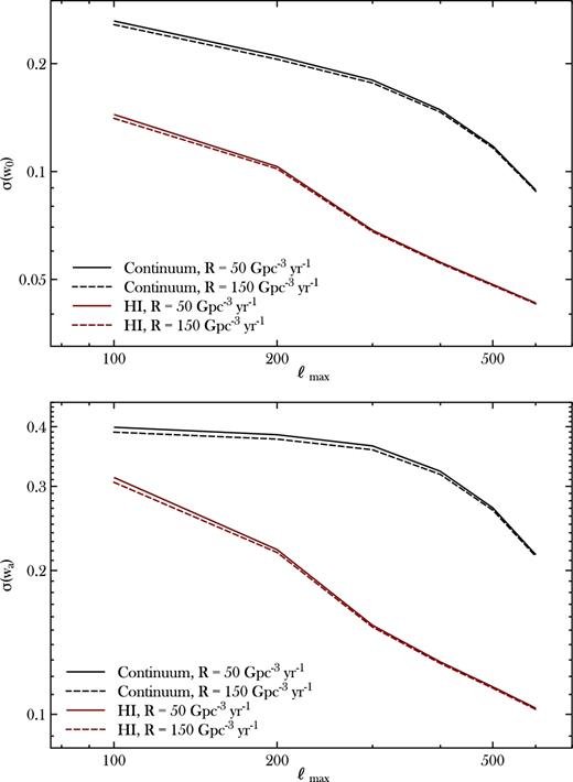
Predicted constraints on dynamical dark energy parameters, as a function of the minimum scale used ℓmax and for two different values of the BBH merger rate R. Black lines show forecasts for continuum surveys, red lines for H i spectroscopic ones.
We use the cross-correlation of foreground galaxies that act as lenses for background GWs. The main shot noise contribution comes from the GW number counts, therefore we select a larger bin for them than the one(s) for galaxies. In the continuum case, given that redshift information will allow only wide bins in z, we correlate a 0 < z < 1 bin of galaxies with a 1 < z < 3 bin of GWs. We show the predicted errors on dark energy parameters for this case with black lines. In the case of the H i surveys, high-precision redshifts will be available, therefore we cross-correlate galaxies from four z-bins with Δz = 0.25 in the range 0 < z < 1, with a background of GWs at 1 < z < 3. Results for this case are shown with red lines.
Results are virtually independent on the flux limits, as results are shot noise limited from the GW bin but will not change once ng in equation (6) is reasonably large.
As expected, the constraining power increases in the case of more bins (and so more correlations); moreover, increasing the maximum multipole used considerably improves the constraining power of this observable, as lensing is more powerful on small scales.
In Fig. 5, we show the same predictions but for the modified gravity parameters of equation (18)–(19); results and considerations about what part of the experiment parameter space increases the constraining power are similar.
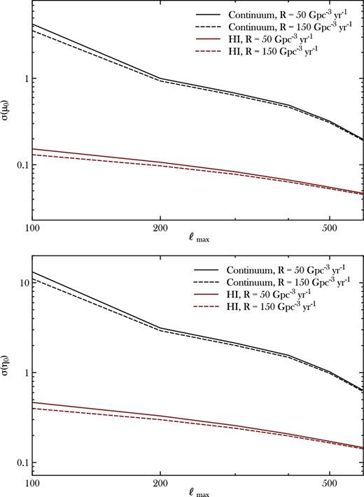
Same as Fig. 4 but for modified gravity parameters.
For dark energy parameters, when using H i surveys, in the case of a conservative ℓmax ≈ 100, constraints will be somewhat comparable to current ones, while in the optimistic case of ℓmax = 600 they will be competitive with current best constraints (Samushia, Percival & Raccanelli 2012; Samushia et al. 2013, 2014; Alam et al. 2016) and even future ones from the combination of CMB and redshift-space distortions (Raccanelli et al. 2015b).
The situation is similar but even more positive for the modified gravity constraints. Our results show that, again, H i surveys will provide better constraints than continuum ones, given the larger number of correlations measured (and small shot noise even when bins are smaller, due to the very large number density of future radio surveys). Even when using ℓmax = 100, measurements of lensing of GWs from radio galaxies could provide constraints stronger than current Planck (Planck Collaboration XIV 2016) and competitive with future (Zhao et al. 2015) limits. However, in this case, increasing ℓmax would allow an improvement in the constraining power that is significative but not dramatic (mostly because in these models, deviations from GR are largest at large scales). Nevertheless, these results show that radial cross-correlations galaxy–GWs can be a very powerful instrument for testing deviations from Einstein's GR.
In any case, any measurements resulting from the cross-correlation galaxy–GW and lensing of GWs will represent a very important, independent and complementary check to results obtained with e.g. galaxy surveys or CMB.
It is important to note that the constraints presented here are purely indicative, and it is likely that a careful optimization could improve them. Possible ways to increase the constraining power can come from a targeted choice of number, width and redshift centre of the bins, the choice of specific galaxy populations with an optimal redshift distribution and bias; additionally, the multitracer technique would improve the constraints by a factor of a few. A detailed investigation of that is however beyond the scope of this paper.
4 GW BACKGROUND
A stochastic gravitational wave background (SGWB) is a key prediction of inflationary cosmology (see e.g. Maggiore 2000), so that its detection is one of the main goals of astrophysics. This can be sought either via direct or indirect measurements, as the presence of the SGWB would have left imprints on different observables.
We can divide the effects of an SGWB on cosmological observables into early- and late-time effects. Early Universe effects include modifications to the BBN process, in particular Deuterium abundance (Pagano, Salvati & Melchiorri 2016) and imprints on the CMB: both temperature and polarization of CMB photons are affected by the SGWB, in particular the formation of a B-mode pattern in the polarization (Kamionkowski, Kosowsky & Stebbins 1997; Seljak & Zaldarriaga 1997; Polnarev, Miller & Keating 2008).
Regarding late-time effects, the presence of a GW background modifies the statistics of primordial curvature perturbations and creates tidal effects that affect clustering of structures (Masui & Pen 2010; Schmidt & Jeong 2012a; Dai, Jeong & Kamionkowski 2013; Schmidt, Pajer & Zaldarriaga 2014). Moreover, the presence of tensor perturbations causes projection effects that change the observed matter density field (Jeong & Schmidt 2012) and causes a distortion of galaxy shapes (Dodelson et al. 2003; Dodelson 2010; Schmidt & Jeong 2012a).
Furthermore, GWs have an effect on local light signals propagating from closer objects; this effect could be captured by pulsar timing array observations (see e.g. Joshi 2013).
A measurement and characterization of the SGWB power spectrum will allow tests of early universe models (even though it has been seen as a possible experimental confirmation for inflation, primordial GWs can also be generated in alternative models such as ekpyrotic models (Ben-Dayan 2016; Ito & Soda 2016)), and constrain fundamental parameters such as the tensor-to-scalar ratio r (Smith, Kamionkowski & Cooray 2006a, 2008). In principle, however, the GW background could be sourced by a variety of events, including not only GWs produced during inflation, but also high-z mergers of compact objects (Regimbau & Mandic 2008; Regimbau 2011; Zhu et al. 2011; Cholis 2016; Dvorkin et al. 2016a,b; Mandic, Bird & Cholis 2016), the non-linear gravitational collapse of DM haloes (Carbone, Baccigalupi & Matarrese 2006), and possibly other phenomena, depending on details of the cosmological model (for a recent review, see Guzzetti et al. 2016).
Therefore, several theoretical and experimental efforts are underway for the direct and indirect measurement of the SGWB. The main observables that are used to try to detect the SGWB are (i) direct detection of GWs; (ii) B-modes of polarization in the CMB; (iii) pulsar timing array experiments; (iv) the anisotropy in the galaxy correlation function; (v) correlations of weak gravitational lensing; (vi) intensity mapping experiments probing the dark ages.
The direct detection of the SGWB will be attempted by a number of ground-based experiments that have been proposed, starting with a planned expansion of the LIGO network, with new LIGO nodes in India (IndIGO; Unnikrishnan 2013) and Japan (KAGRA; Aso et al. 2013). Future GW detectors include the ET (Punturo et al. 2010) and the space instrument eLISA (Klein et al. 2016). However, these instruments could detect the SGWB only in the case of non-single-field slow-roll inflation models, that predict a blue inflationary power spectrum (Guzzetti et al. 2016). In order to detect a scale-invariant inflationary power spectrum, more futuristic instruments (Crowder & Cornish 2005), such as the planned DECI-Hertz Interferometer Gravitational wave Observatory (DECIGO; Kawamura et al. 2011) and BBO (Corbin & Cornish 2006), designed primarily to detect the primordial SGWB, are required (Moore, Cole & Berry 2015).
As for the indirect detection, several ground-, balloon- and space-based CMB polarization experiments are under construction or have been proposed (Crill et al. 2008; Bouchet et al. 2011; Kogut et al. 2011; Eimer et al. 2012; Matsumura et al. 2013; Ade et al. 2014; André et al. 2014; Calabrese et al. 2014), and pulsar timing array experiments are underway (McLaughlin 2013; Manchester et al. 2013; Janssen et al. 2015; Lentati et al. 2015).
Current observational upper limits on ΩGW include (i) the constraint ΩGW ≲ 10−13 for 10−17Hz ≲ f ≲ 10−16 Hz from large angular scale fluctuations in the cosmic microwave background temperature (Buonanno 2007); (ii) the combination of cosmological nucleosynthesis and cosmic microwave background constraint gives ΩGW(f) ≲ 10−5 for f ≳ 10−15 Hz (Smith, Pierpaoli & Kamionkowski 2006b; Pagano, Salvati & Melchiorri 2016); (iii) the pulsar timing limit provided by EPTA, ΩGW < 1.2 × 10⁻⁹ for f = 2.8 × 10⁻⁹ Hz (Lentati et al. 2015); (iv) joint analysis of LIGO and Virgo provides an upper limit of ΩGW < 5.6 × 10⁻⁶ for f ∼ 100 Hz (Aasi et al. 2014), and the most recent aLIGO analysis gave |$\Omega _{\rm GW} = 1.1_{-0.9}^{+2.7} \times 10^{-9}$| for f = 25 Hz (Abbott et al. 2016b) and ΩGW < 1.7 × 10⁻⁷ for f = 20–85 Hz (Abbott et al. 2017); (v) limits from very long baseline interferometry radio astrometry of quasars of ΩGW ≲ 10−1 for 10−17 Hz ≲ f ≲ 10−9 Hz (Gwinn et al. 1997) and ΩGW ≲ 4 × 10⁻³ for f ≲ 10−9 Hz (Titov, Lambert & Gontier 2011); (vi) ΩGW ≲ 10−3 for 10−16 Hz ≲ f ≲ 10−10 Hz from the observed galaxy correlation function (Linder 1988). In Fig. 6, we show these constraints in a plot as an illustration.
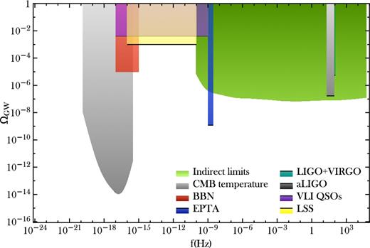
Current constraints on the stochastic GW background.
From CMB data, the joint analysis of Planck, BICEP2 and Keck Array data provides an upper bound of r0.05 < 0.09 at 95 per cent C.L. at frequencies f ∼ 10−17 Hz (Ade et al. 2016).
For more details on the SGWB, see the review articles Allen (1997); Maggiore (2000); Buonanno (2007), and more recently Guzzetti et al. (2016); for a recent review on the search of GWs from inflation using the CMB, see Kamionkowski & Kovetz (2016).
In this paper, we focus on effects of the SGWB on the LSS; a background of GWs will leave an imprint in the angular correlation of galaxies on large scales, and introduce correlations of galaxy shapes. However, LSS measurements will provide weaker constraints than the CMB. Realistically, CMB experiments will measure r, and if its value is not negligible (around the upper limit of current constraints), LSS could confirm or at least support those measurements.
4.1 Cosmometry
As suggested by Linder (1986); Braginsky et al. (1990); Kaiser & Jaffe (1997), a stochastic GW background causes the apparent positions of distant sources to fluctuate, with angular deflections of order the characteristic strain amplitude of the GWs, and these fluctuations may be detectable with high-precision astrometry. Estimates of the upper limits obtainable on the GW spectrum ΩGW(f), at frequencies of order f ∼ 1 yr−1 are available in literature, and they generally predict constraints comparable with the ones from pulsar timing (see e.g. Jaffe 2004; Book & Flanagan 2011).
In this paper, we extend those predictions to future radio surveys and try to understand what are the instrument requirements needed to make cosmological radio galaxy high-z astrometry, which we call ‘cosmometry’, competitive with other methods and possibly have a detection of the effects of an SGWB.
4.1.1 Effect of an SGWB on galaxy positions
Here, we investigate limits on ΩGW that will be possible to set by using cosmometry from future radio surveys. In Figs 7 and 8, we show predicted upper limits on ΩGW as a function of angular resolution, observing time and number of objects observed. We focus on GWs with a period of 1 year. We also indicate the SKA VLBI configuration in two different configurations, where we call SKAVLBI-1 a survey detecting 107 objects and SKAVLBI-2 a survey detecting 109 objects, in both cases with an angular resolution of 10 μarcsec and over 10 yr of observations. Different models of inflation predict different amplitude and scale dependence of the SGWB (see e.g. Guzzetti et al. 2016). As can be seen from Fig. 6, cosmometry constraints could be competitive with current ones, but it would be difficult to reach the single field slow-roll inflation prediction of ∼10−15. However, the background due to primordial or supermassive black hole binaries could be detected (see e.g. Abbott et al. 2017; Clesse & García-Bellido 2016).

Predicted precision in the measurements of ΩGW from cosmometry analyses, as a function of the number of objects and years of observation, assuming an angular resolution of 10 μarcsec. See text for the details about the assumed experiment.
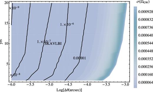
As in Fig. 7 but as a function of the angular resolution and years of observation, assuming 107 objects. See text for the details about the assumed experiment.
We can see that, in order to detect the SGWB from changes in galaxy positions, extremely precise measurements will be needed. Even with a very optimistic SKA in VLBI configuration, a detection of GWs from inflation is virtually out of reach. However, configurations with baseline lengths up to 10 000 km in length are being considered (Paragi et al. 2015), therefore very precise measurements might be possible in a (relatively) near future. In any case, limits set with this methodology are complementary to the ones set by e.g. direct detection of GWs, making results from forthcoming instruments useful and interesting.
4.2 Cosmic rulers
In this section, we investigate the possibility of using LSS standard rulers to detect the effects of a background of GWs; we make use of the ‘cosmic rulers’ formalism (Schmidt & Jeong 2012b), and investigate if future radio surveys will be able to detect the SGWB by using either the anisotropy of the two-point galaxy correlation or galaxy ellipticities, as first suggested by Jeong & Schmidt (2012); Schmidt & Jeong (2012a). We will briefly review the methodology introduced in the above series of paper, that we will use to obtain our results, and then show forecasts for measurements that will be possible to obtain with future radio surveys. Note that, apart from a slightly different notation and some rearrangements, all the results here coincide with the ones in the cited ‘cosmic rulers’ series. For a direct translation between the two notations, one can compare Bertacca et al. (2012) with Jeong, Schmidt & Hirata (2012).
4.2.1 Galaxy clustering
In the context of a general relativistic description of the observed galaxy clustering (see e.g. Yoo, Fitzpatrick & Zaldarriaga 2009; Bertacca et al. 2012; Jeong, Schmidt & Hirata 2012), a series of effects need to be considered as corrections to the standard, Newtonian, formalism, which includes only scalar perturbations to the matter density field and redshift-space distortions (RSD). In a similar way, GWs (tensor perturbations) affect, on the largest scales, the clustering statistics via volume and magnification effects.
Differences in the effect of tensor perturbations from scalar ones were first noted in Kaiser & Jaffe (1997): in particular, tensor modes redshift away, so that their contribution to the clustering of LSS tracers is dominated by contributions close to the time of emission; instead, scalar perturbations grow, and the deflection is amplified by transverse modes (Jeong & Schmidt 2012).
GWs are waves in the transverse (∂ihij) and traceless (|$h^i_{\,i}$|) components of the metric perturbation, defined in the FRW Universe in terms of the spatial components of the metric by gij = a2(δij + 2hij).
Throughout, we will assume a tensor-to-scalar ratio of r = 0.09 at k* (consistent with current upper limits), which together with our fiducial cosmology determines the amplitude |$\Delta _T^2$|.
Errors in the angular correlations are computed as in equation (6), and they are proportional to the amplitude of the correlations, cosmic variance and the number density of objects. Hence, given a galaxy survey, the best chance to detect the effect of tensor perturbations would be, as pointed out in Jeong & Schmidt (2012), by looking at the effects on radial cross-bin correlations. In the context of the full observed galaxy correlations, radial correlations are dominated by cosmic magnification terms (Raccanelli et al. 2016b), that can be orders of magnitude larger than the Newtonian prediction (Raccanelli et al. 2016d). However, magnification terms depend on the magnification bias s; therefore, if one selects a sample of galaxies with s = 0.4, it is clear from equation (11) that the magnification contribution is cancelled. Moreover, as mentioned above, tensor perturbation effects on LSS are larger closer to the time of emission, so that high-redshift bins are the most useful. Therefore, radio continuum surveys with the CBR technique provides the ideal scenario.
Unfortunately, even in the most optimistic cases with high-z sources and small shot noise, tensor perturbations remain undetectable. In Fig. 9, we show the signal-to-noise ratio, defined as |$(C_\ell ^{\rm tot}-C_\ell ^{\mathfrak {t}})/\sigma _{C_\ell }$|, for the case of the Slim = 1 nJy continuum survey. As pointed out above, radial cross-bin correlations at high-z are the most promising ways to detect this signal, so we computed forecasts by using radio continuum surveys with five bins centred at z = {2, 3, 4, 5, 6}. The plot shows the SNR for the first 20 multipoles ℓ, for different cross-bin radial correlations.
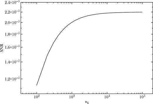
Signal-to-noise ratio for tensor perturbation contributions (assuming r = 0.09) to the observed galaxy two-point correlation function.
Our results show that even in the case of negligible shot noise and high-z correlations, the total SNR achievable will not reach 0.0001. While in principle the multi-tracer technique and optimization on the number of bins, galaxy populations, bias and other parameters can significantly increase the SNR, it appears clear that it is very unlikely any survey built in the foreseeable future could allow a robust measurement using this observable.
4.2.2 Clustering fossils
In principle, another way of measuring effects from primordial GWs has been developed in Jeong & Kamionkowski (2012); Dai et al. (2016), where it is shown how to search a galaxy survey for the imprint of primordial scalar, vector, and tensor fields. However, such effects require an extremely futuristic galaxy survey and measurements in the highly non-linear regime or higher order correlations; in this paper, we do not focus on detailed modelling of non-linearities nor higher order correlations, hence we leave a careful investigation of this formalism to a future work.
4.2.3 Weak lensing
Now we turn our focus on effects of tensor perturbations on the correlation of galaxy ellipticities, referring again to the ‘cosmic rulers’ formalism, and in particular we follow Schmidt & Jeong (2012a); Schmidt et al. (2014). In the unperturbed case, one would expect galaxy ellipticities to be uncorrelated, but unlike in the case of the galaxy correlation function, shear is a tensorial quantity, and thus there is a possible intrinsic contribution correlated with the GW background; this can be thought as analogous to the intrinsic alignment effect present for scalar perturbations. Scalar perturbations contribute only to the E-mode component (at linear order), while tensor perturbations also contribute to the B-mode. Hence, the curl-mode of the correlation of galaxy ellipticities can be used to detect a stochastic GW background. In the rest of this section, we summarize what is the effect of a background of GWs to the correlation of ellipticities, and study what are the minimum experiment configurations required to detect the effect of such background, assuming r = 0.09.
The results are obtained by calculating the combined SNR of correlations of |$C_\gamma ^{BB}(\ell )$| at redshift bins centred at z = {2, 3, 4, 5, 6, 7, 8}, assuming an almost flat N(z) as in the continuum 1 nJy case of Fig. 1. In Fig. 10, we show the combination of σe and |$\bar{n}_g$| required to have a 1σ detection of the GW background with r = 0.09.
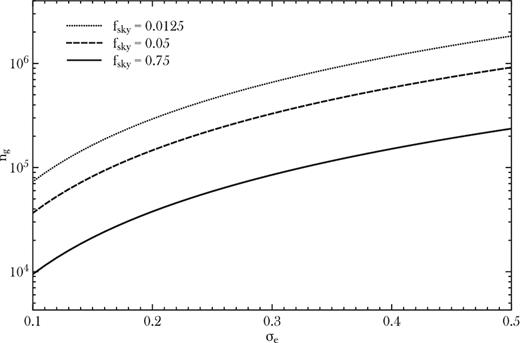
Minimum number of galaxies per deg2 per bin needed to detect GWs from inflation with r = 0.09, using the correlation of galaxy ellipticities, as a function of intrinsic ellipticity error σe, for three different sky coverage values. See text for details.
We compute our results for three different survey areas, fsky = {0.0125, 0.05, 0.75}. Of course, a smaller area surveyed would require a larger minimum number density, but very large number densities could be more easily achievable with dedicated deep surveys focusing on a smaller part of the sky.
In any case, for futuristic surveys as in Fig. 1, the most optimistic case used in this paper predicts around 104 sources per deg2, meaning that in order to have such detection, a survey should observe a total of ∼105 objects above z = 2, with σe ≈ 0.1 over 75 per cent of the sky, making it a very difficult target but somewhat more doable than the galaxy clustering case.
5 CONCLUSIONS
This work analysed a few possible ways to achieve this goal: by cross-correlating radio galaxy catalogues with GW maps, it is possible to determine properties of the progenitors of merging black hole binaries and forecast how the magnification of GWs by foreground radio sources allows us to test models that explain cosmic acceleration. Furthermore, it is in principle possible to detect the effects of a background of GWs, by measuring angular motion and large-scale correlations of galaxy distribution and lensing.
By using simulated catalogues resembling planned instruments, it was possible to show that the angular galaxy–GW cross-correlation can set stringent limits on properties of the progenitors of BBHs, testing formation models and the possibility that primordial black holes are in fact the dark matter.
Radial cross-correlations can be used to detect the magnification bias of GWs that are lensed by low-redshift galaxies, and future laser interferometers, paired with forthcoming radio galaxies, can provide constraints on dynamical dark energy and modified gravity parameters that are competitive with the ones obtained with galaxy surveys alone and in combination with the CMB.
On the other hand, the detection of a stochastic GW background on galaxy position and distribution presents a much greater challenge. Tensor perturbation effects on galaxy clustering remain orders of magnitude below errors in measurements of galaxy power spectra, even in the case of very futuristic galaxy surveys. The situation is slightly more optimistic for the correlation of lensing effects: in the case of a deep, full-sky survey with very precise shape measurements, it will be possible to measure the SGWB (provided that the tensor-to-scalar ratio r is not negligibly small). In any case, any measurements of GW effects coming from radio galaxy surveys or their correlation with GW detectors, would represent a valuable cross-check of other measurements and potentially provide new insights about cosmological models of current interest.
In summary, radio galaxy surveys can be used to provide information useful for GW astronomy and contribute studying the Universe in a new and complementary way.
Acknowledgments
I am indebted to Ely Kovetz for encouraging the development of this project and carefully reading the manuscript. I would like to thank Yacine Ali-Haïmoud, Ilias Cholis, Julian Munoz, Gianfranco de Zotti, Maria Chiara Guzzetti, Raul Jimenez and Licia Verde for commenting on the manuscript; Daniele Bertacca, Stefano Camera, Marc Kamionkowski, Sabino Matarrese, Prina Patel for useful discussions. I am supported by the John Templeton foundation.
CMB measurements have tentatively closed this window (Ricotti, Ostriker & Mack 2008), but the result is based on several untested assumptions and until a more detailed modelling is used, one should associate a large uncertainty with this limit. Hence, we defer this issue to further studies.
REFERENCES
