


Abstract
Emission geometries, including emission region heights, beam shapes and radius-to-frequency mapping, are important clues for pulsar radiation models. Multiband radio observations reveal this valuable information. In this paper, we study two bright pulsars, PSRs B0329+54 and B1642−03, and observe them at high frequencies: 2.5, 5 and 8 GHz. The newly acquired data, together with historical archives, provide an atlas of multifrequency profiles spanning from 100 MHz to 10 GHz. We study the frequency evolution of pulse profiles as well as radiation regions using these data. First, we fit the pulse profiles with Gaussian functions to determine the phase of each component, and then we calculate the radiation altitudes of different emission components and radiation regions. We find that the inverse Compton scattering (ICS) model can reproduce the radiation geometry of these two pulsars. However, for PSR B0329+54, the radiation can be generated in either an annular gap (AG) or a core gap (CG), while the radiation of PSR B1642−03 can only be generated in a CG. This difference is caused by the inclination angle and the impact angle of these two pulsars. The relationship between the beaming angle (the angle between the radiation direction and the magnetic axis) and the radiation altitude versus frequency is also presented by modelling the beam–frequency evolution in the ICS model. The multiband pulse profiles of these two pulsars can be described well by the ICS model combined with the CG and AG.
1 INTRODUCTION
Since the first pulsar was discovered in 1967 (Hewish et al. 1968), more than 2600 radio pulsars1 (Manchester et al. 2005) and 205 gamma-ray pulsars2 have been discovered. A variety of models have been proposed to explain their radiation processes (Beskin et al. 2015). However, until now, there has still been a question concerning pulsar radiation. Goldreich & Julian (1969) proposed that a rotating magnetic neutron star holds a charge-separated magnetosphere. Sturrock (1971) quickly realized that a photon with energy larger than 2mec2 can generate electron–positron pairs to produce radio emission by curvature radiation (CR). Since then, Ruderman & Sutherland (1975) have developed the Sturrock model. They have proposed that the first accelerating model, which is called the RS model, presents an accelerated region – a core gap (CG) model – above the polar cap of the pulsar to accelerate particles. These particles move out along the curved open magnetic field lines to produce radiation.
In recent years, Qiao et al. (2004) have presented other accelerating region models, such as the annular gap (AG) model, to understand particle acceleration. Qiao et al. (2004) have suggested that there is an AG accelerating region above the polar cap of pulsars around the CG. The boundary of the CG and the AG is the critical field line (CFL; Holloway 1975). In these two regions, radio emission is believed to be generated by an inverse Compton scattering (ICS) process between secondary relativistic particles and low-frequency waves (Qiao 1988a,b; Zhang & Qiao 1996; Qiao & Lin 1998). The ICS model can explain the pulse profiles with peaks numbering from one to five (Qiao & Lin 1998; Zhang et al. 2007), widening or narrowing profiles with increasing frequency, ‘mode changing’ behaviour (Qiao & Zhang 1996; Zhang, Qiao & Han 1997a; Zhang et al. 1997b) and polarization (Xu, Qiao & Han 1997; Xu et al. 2000; Xu, Qiao & Han 2001). In addition, this model, combined with the CG and the AG, can explain many observational phenomena at high-energy bands (Qiao et al. 2004; Lee et al. 2006a,b, 2009, 2010; Du et al. 2010, 2011; Du, Qiao & Wang 2012; Du, Qiao & Chen 2013; Du et al. 2015).
Multiband observations of pulsar are an effective tool for testing and constraining theoretical models. By analysing the observed multifrequency pulse profiles, the location, geometry and spectrum of pulsar emissions can then be determined so as to constrain theoretical models. In order to empirically classify the observational properties of radio pulsars, Rankin (1983, 1993) proposed that a radio beam usually consists of two hollow cones and a quasi-axial core. The debate between ‘core-cone’ beam models and other models (such as ‘patchy’ beams, fan beams, microbeam patterns, etc.) as well as multifrequency observed data has continued between many authors (e.g. Lyne & Manchester 1988; Kramer et al. 1994; Manchester 1995; Gil & Krawczyk 1996; Melrose & Gedalin 1999; Mitra & Deshpande 1999; Gangadhara & Gupta 2001; Han & Manchester 2001; Kijak & Gil 2002; Manchester et al. 2005; Karastergiou & Johnston 2007; Maciesiak & Gil 2011; Maciesiak, Gil & Ribeiro 2011; Maciesiak, Gil & Melikidze 2012; Beskin & Philippov 2012; Wang, Wang & Han 2012; Fonseca et al. 2014; Wang et al. 2014; Cerutti, Philippov & Spitkovsky 2016; Dyks et al. 2016; Pierbattista et al. 2016; Teixeira et al. 2016). Besides, some theoretical perspectives – for example, radio radiation beams are hollow and lack a core cone and pulse profiles at lower frequencies are wider than those at higher frequencies – have been challenged by a large number of observations. The great variety of pulse profiles and their frequency evolution indicate the high complexity of pulsar beam patterns.
The multifrequency pulse profile characteristics of PSRs B0329+54 and B1642−03 challenge some theoretical models (e.g. the CR model). PSR B0329+54 is one of the brighter pulsars in the northern sky. It has a spin period of P = 0.715 s (Hobbs et al. 2004). The pulse profiles of PSR B0329+54 have obvious central peaks (Rankin 1983, 1993), and the form of mean pulse profiles shows five (Kramer 1994) or even nine components (Gangadhara & Gupta 2001; Gupta & Gangadhara 2003; Chen et al. 2011). The pulse profiles of this pulsar show narrower profiles at higher frequencies. PSR B1642−03 has a spin period of P = 0.388 s (Manchester et al. 2005). The pulse profiles of PSR B1642−03 consist of a core and an inner cone component, and the pulse profiles at higher frequencies are wider than those at lower frequencies (Rankin 1983, 1993; Kramer 1994). The observed profile properties of these two pulsars can hardly be understood in certain theoretical models, such as the CR model. Furthermore, as far as we know, no attempt has been made to understand a broad-band pulse profile evolution within the framework of most models. Therefore, it is of great significance to carry out more multiband observations of pulse profiles in order to test and constrain pulsar radiation mechanism models.
The major aim of this paper is to investigate the evolution of pulse profiles over a frequency range of the order of 2 mag, and to study the pulsar radio radiation model, particularly the ICS model. In Section 2, we present the observed data of these sources collected from the on-line data base and the new observations by the Kunming 40-m telescope at the Yunnan Astronomical Observatory, Chinese Academy of Sciences (CAS) and by the Tianma 65-m telescope at the Shanghai Astronomical Observatory, CAS. In Section 3, we separate the emission components of the integrated pulse profiles of PSRs B1642−03 and B0329+54 by Gaussian fitting, we calculate their radiation altitudes and we present the radio radiation regions of these two sources. We give a discussion and our conclusions in Section 4.
2 OBSERVATION AND DATA REDUCTION
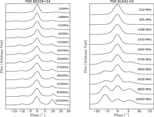
Multiband pulse profiles are very important for a detailed study of the frequency evolution of pulse profiles. For PSR B0329+54, there are 10 profiles at frequencies 143, 408, 610, 925, 1642, 1410, 4750, 4850, 8500 and 10 550 MHz (Kramer 1994; von Hoensbroech & Xilouris 1997; Gould & Lyne 1998; Pilia et al. 2016), while for PSR B1642−03, there are eight profiles at frequencies 610, 925, 1408, 1410, 1642, 4850, 4750 and 10 550 MHz (Seiradakis et al. 1995; von Hoensbroech & Xilouris 1997; Gould & Lyne 1998). The frequencies for PSR B1642−03 were obtained through the European Pulsar Network data base.3 In order to provide more profiles for the purpose of constraining theoretical models, we made observations of three profiles at frequencies 2256, 5030 and 8600 MHz. The pulse profiles at frequencies 5030 and 8600 MHz were obtained from observations using the Tianma 65-m telescope at the Shanghai Astronomical Observatory, CAS, at longitude 121|$_{.}^{\circ}$|1 E and latitude +30|$_{.}^{\circ}$|9 N. The data were folded through the Digital Backend System (Yan et al. 2015). The pulse profile at frequency 2256 MHz was obtained from observations using the Kunming 40-m telescope at the Yunnan Astronomical Observatory, CAS, at longitude 102|$_{.}^{\circ}$|8 E and latitude 25|$_{.}^{\circ}$|0 N (Hao et al. 2010). The data were folded through the Pulsar Digital Filter Bank 3 with parameters provided by psrcat,4 version 1.51 (Manchester et al. 2005). The radio-frequency interference (RFI) was removed manually with the software package psrchive5 (Hotan, van Straten & Manchester 2004; van Straten, Demorest & Oslowski 2012). The observed information is listed in Table 1.
Observational information.
| Center frequency (MHz) | Telescope | Bins | Bandwidth (MHz) | System temperature (K) | SEFDa (Jy) | Duration (s) |
|---|---|---|---|---|---|---|
| 2256 | Kunming 40 mb | 512 | 251.5 | 80 | 350 | 13035.326 |
| 5030 | Tianma 65 mc | 1024 | 800 | 20 | 25 | 1773.823 |
| 8600 | Tianma 65 mc | 1024 | 800 | 35 | 50 | 3600 |
3 MULTIBAND PROFILE ANALYSIS IN THE ICS MODEL
The beam shape and the acceleration regions are very important in order to constrain pulsar emission mechanisms. The emission beam contains two or three components, a centre cone (the core cone) and one or two nested cones (the inner and outer cones). We obtain the pulse profile when the emission beam sweeps across the line of sight. The core component and the inner and outer cone components correspond to the central peak and the peaks on the outside of the pulse profiles, respectively. Each component of the pulse profile is assumed to have a Gaussian shape and can be separated by Gaussian fitting (Wu, Xu & Rankin 1992; Kramer 1994; Wu et al. 1998). The cross-section structure of the emission beam can be deduced by the average pulse profile (Oster & Sieber 1977; Rankin 1983; Manchester 1995; Qiao & Lin 1998; Han & Manchester 2001). In the magnetosphere of pulsar, the open field line region is divided into two parts by the CFL. One part containing the magnetic axis is called the CG (Ruderman & Sutherland 1975) and the other part is the AG (Qiao et al. 2003a,b, 2004, 2007). The locations and shapes of the particle acceleration regions (CG and AG) above the polar cap can be determined by calculating the radiation altitude r (the distance from the pulsar centre to the radiation point) of each component of the pulse profile and the beaming angle θμ (the angle between the radiation direction and the magnetic axis).
3.1 Component separation with Gaussian fitting

Gaussian fitting of PSR B0329+54 multifrequency profiles. The black dots correspond to the observation data. Red solid and blue dashed lines correspond to the fitting curves and single Gaussian, respectively. Pink dots denote the residuals. The maximum pulse flux is normalized, and the profiles are aligned at the position of the central peak.
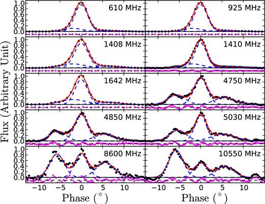
As for Fig. 1, but for PSR B1642−03.
Fitting curve evolution versus observation frequency.
Gaussian fitting parameters of PSR B0329+54. Note that f is the observing frequency and Ii, pi and wi are the intensity, peak position and standard deviation of the ith Gaussian component, respectively.
| f | i | pi | Ii | wi |
|---|---|---|---|---|
| (MHz) | ||||
| 143 | 1 | −16.767 ± 0.07 | 0.056 ± 0.002 | 1.766 ± 0.07 |
| 2 | −3.838 ± 0.19 | 0.126 ± 0.003 | 2.667 ± 0.13 | |
| 3 | 0.0 | 0.96 ± 0.01 | 1.322 ± 0.01 | |
| 4 | 4.208 ± 0.17 | 0.024 ± 0.003 | 1.126 ± 0.19 | |
| 5 | 11.769 ± 0.05 | 0.114 ± 0.002 | 2.604 ± 0.05 | |
| 408 | 1 | −13.397 ± 0.03 | 0.053 ± 0.001 | 1.262 ± 0.03 |
| 2 | −3.47 ± 0.06 | 0.148 ± 0.003 | 1.906 ± 0.05 | |
| 3 | 0.0 | 0.951 ± 0.004 | 1.299 ± 0.004 | |
| 4 | 3.395 ± 0.62 | 0.023 ± 0.001 | 5.788 ± 0.31 | |
| 5 | 9.847 ± 0.02 | 0.101 ± 0.001 | 1.27 ± 0.021 | |
| 610 | 1 | −12.53 ± 0.03 | 0.084 ± 0.001 | 1.57 ± 0.03 |
| 2 | −1.602 ± 0.17 | 0.295 ± 0.01 | 3.169 ± 0.07 | |
| 3 | 0.0 | 0.733 ± 0.01 | 1.308 ± 0.01 | |
| 4 | 7.377 ± 0.98 | 0.052 ± 0.003 | 3.651 ± 0.58 | |
| 5 | 9.606 ± 0.04 | 0.086 ± 0.01 | 1.209 ± 0.07 | |
| 925 | 1 | −11.966 ± 0.04 | 0.114 ± 0.002 | 1.581 ± 0.04 |
| 2 | −1.586 ± 0.33 | 0.335 ± 0.02 | 3.267 ± 0.14 | |
| 3 | 0.0 | 0.695 ± 0.02 | 1.301 ± 0.02 | |
| 4 | 6.84 ± 1.06 | 0.099 ± 0.01 | 3.37 ± 0.50 | |
| 5 | 9.486 ± 0.04 | 0.134 ± 0.01 | 1.208 ± 0.07 | |
| 1410 | 1 | −11.427 ± 0.04 | 0.159 ± 0.004 | 1.479 ± 0.04 |
| 2 | −1.123 ± 0.09 | 0.439 ± 0.01 | 3.281 ± 0.05 | |
| 3 | 0.0 | 0.585 ± 0.01 | 1.055 ± 0.02 | |
| 4 | 7.719 ± 0.23 | 0.152 ± 0.01 | 2.751 ± 0.15 | |
| 5 | 9.482 ± 0.03 | 0.17 ± 0.01 | 0.847 ± 0.05 | |
| 1642 | 1 | −11.365 ± 0.04 | 0.182 ± 0.004 | 1.596 ± 0.04 |
| 2 | −1.326 ± 0.18 | 0.495 ± 0.02 | 3.291 ± 0.09 | |
| 3 | 0.0 | 0.541 ± 0.02 | 1.18 ± 0.03 | |
| 4 | 7.338 ± 0.52 | 0.163 ± 0.01 | 2.962 ± 0.29 | |
| 5 | 9.375 ± 0.04 | 0.204 ± 0.02 | 1.08 ± 0.07 | |
| 2256 | 1 | −11.007 ± 0.05 | 0.173 ± 0.004 | 1.604 ± 0.05 |
| 2 | −1.298 ± 0.15 | 0.518 ± 0.02 | 3.188 ± 0.07 | |
| 3 | 0.0 | 0.516 ± 0.02 | 1.162 ± 0.03 | |
| 4 | 7.492 ± 0.44 | 0.159 ± 0.01 | 2.896 ± 0.26 | |
| 5 | 9.401 ± 0.05 | 0.182 ± 0.02 | 1.006 ± 0.07 | |
| 4750 | 1 | −10.542 ± 0.05 | 0.103 ± 0.003 | 1.708 ± 0.05 |
| 2 | −1.409 ± 0.18 | 0.531 ± 0.04 | 2.423 ± 0.06 | |
| 3 | 0.0 | 0.514 ± 0.04 | 1.341 ± 0.04 | |
| 4 | 6.481 ± 0.73 | 0.099 ± 0.003 | 3.754 ± 0.41 | |
| 5 | 9.423 ± 0.03 | 0.183 ± 0.01 | 0.988 ± 0.04 | |
| 4850 | 1 | −10.25 ± 0.02 | 0.121 ± 0.001 | 1.629 ± 0.02 |
| 2 | −1.403 ± 0.07 | 0.458 ± 0.01 | 2.586 ± 0.02 | |
| 3 | 0.0 | 0.579 ± 0.01 | 1.372 ± 0.01 | |
| 4 | 6.987 ± 0.24 | 0.099 ± 0.001 | 3.6 ± 0.15 | |
| 5 | 9.617 ± 0.01 | 0.223 ± 0.003 | 0.959 ± 0.01 | |
| 5030 | 1 | −10.262 ± 0.05 | 0.109 ± 0.002 | 1.768 ± 0.05 |
| 2 | −1.156 ± 0.06 | 0.548 ± 0.01 | 2.505 ± 0.03 | |
| 3 | 0.0 | 0.492 ± 0.01 | 1.149 ± 0.02 | |
| 4 | 7.734 ± 0.26 | 0.097 ± 0.004 | 3.35 ± 0.20 | |
| 5 | 9.6 ± 0.02 | 0.196 ± 0.01 | 0.847 ± 0.03 | |
| 8500 | 1 | −9.037 ± 0.16 | 0.093 ± 0.01 | 1.942 ± 0.18 |
| 2 | −0.352 ± 0.08 | 0.578 ± 0.09 | 2.184 ± 0.12 | |
| 3 | 0.0 | 0.413 ± 0.09 | 1.167 ± 0.10 | |
| 4 | 8.132 ± 0.74 | 0.076 ± 0.01 | 3.717 ± 0.58 | |
| 5 | 10.483 ± 0.04 | 0.244 ± 0.01 | 0.858 ± 0.05 | |
| 10 550 | 1 | −9.255 ± 0.08 | 0.111 ± 0.01 | 1.338 ± 0.08 |
| 2 | −0.098 ± 0.07 | 0.318 ± 0.04 | 2.861 ± 0.16 | |
| 3 | 0.0 | 0.676 ± 0.04 | 1.273 ± 0.04 | |
| 4 | 9.765 ± 0.18 | 0.125 ± 0.02 | 2.86 ± 0.28 | |
| 5 | 9.899 ± 0.02 | 0.522 ± 0.02 | 1.035 ± 0.03 |
Gaussian fitting parameters of PSR B1643−03. The parameters are the same as in Table 2.
| f | i | pi | Ii | wi |
|---|---|---|---|---|
| (MHz) | ||||
| 610 | 1 | −1.895 ± 2.52 | 0.114 ± 0.12 | 2.136 ± 0.73 |
| 2 | 0.0 | 0.946 ± 0.17 | 1.523 ± 0.05 | |
| 3 | 5.427 ± 0.76 | 0.034 ± 0.003 | 3.069 ± 0.48 | |
| 925 | 1 | −1.894 ± 2.35 | 0.114 ± 0.11 | 2.136 ± 0.68 |
| 2 | 0.0 | 0.946 ± 0.16 | 1.523 ± 0.05 | |
| 3 | 5.427 ± 0.71 | 0.034 ± 0.003 | 3.069 ± 0.45 | |
| 1408 | 1 | −1.991 ± 0.76 | 0.144 ± 0.03 | 2.886 ± 0.25 |
| 2 | 0.0 | 0.877 ± 0.04 | 1.619 ± 0.02 | |
| 3 | 5.664 ± 0.65 | 0.067 ± 0.01 | 3.249 ± 0.31 | |
| 1410 | 1 | −1.908 ± 0.99 | 0.145 ± 0.04 | 2.437 ± 0.33 |
| 2 | 0.0 | 0.886 ± 0.07 | 1.397 ± 0.04 | |
| 3 | 5.914 ± 0.88 | 0.048 ± 0.004 | 3.191 ± 0.57 | |
| 1642 | 1 | −1.896 ± 1.18 | 0.177 ± 0.05 | 2.959 ± 0.43 |
| 2 | 0.0 | 0.881 ± 0.07 | 1.471 ± 0.05 | |
| 3 | 6.201 ± 1.06 | 0.074 ± 0.01 | 2.778 ± 0.61 | |
| 4750 | 1 | −5.641 ± 0.08 | 0.34 ± 0.01 | 1.973 ± 0.09 |
| 2 | 0.0 | 0.937 ± 0.01 | 1.529 ± 0.04 | |
| 3 | 5.589 ± 0.15 | 0.247 ± 0.01 | 2.314 ± 0.15 | |
| 4850 | 1 | −5.526 ± 0.07 | 0.346 ± 0.01 | 1.877 ± 0.07 |
| 2 | 0.0 | 0.939 ± 0.01 | 1.506 ± 0.03 | |
| 3 | 5.497 ± 0.12 | 0.25 ± 0.01 | 2.281 ± 0.13 | |
| 5030 | 1 | −5.344 ± 0.07 | 0.38 ± 0.01 | 1.942 ± 0.08 |
| 2 | 0.0 | 0.912 ± 0.02 | 1.329 ± 0.03 | |
| 3 | 5.202 ± 0.20 | 0.239 ± 0.01 | 2.709 ± 0.20 | |
| 8600 | 1 | −5.697 ± 0.08 | 0.829 ± 0.03 | 1.693 ± 0.08 |
| 2 | 0.0 | 0.839 ± 0.03 | 1.482 ± 0.10 | |
| 3 | 5.578 ± 0.16 | 0.533 ± 0.03 | 2.102 ± 0.17 | |
| 10 550 | 1 | −5.798 ± 0.06 | 0.961 ± 0.03 | 1.676 ± 0.07 |
| 2 | 0.0 | 0.5 ± 0.03 | 1.542 ± 0.16 | |
| 3 | 5.665 ± 0.20 | 0.393 ± 0.02 | 2.069 ± 0.21 |
For PSR B0329+54, the integrated profiles can be separated into five (Kramer 1994) or even nine components (Gangadhara & Gupta 2001). In this work, however, we fit each observational pulse profile with five Gaussian components. For PSR B1642−03, we fit each pulse profile with three Gaussian components to obtain satisfied residual. As the fitting results in Figs 1–3 indicate, the integrated pulse profiles for PSR B0329+54 show narrower profiles at higher frequencies. Each integrated pulse profile of PSR B1642−03 has only a core and one inner cone component, and the pulse profiles at higher frequencies are wider than those at lower frequencies. These results coincide with the prediction by Qiao & Lin (1998) and Qiao et al. (2001) that slow-rotation pulsars prefer to be double-cone pulsars, whereas fast-rotation pulsars tend to show triple profiles.
3.2 Beam–frequency evolution
We geometrically calculated the different radiation altitudes of components in various frequencies, and simulated the evolutions of radiation altitudes and beaming angles versus frequency in the ICS model. First, the magnetic field of the pulsar was assumed to be dipole with the last open field line (LOF) tangential to the light cylinder; see Zhang et al. (2007) for detailed equations. Secondly, the radiation was assumed to come from the open magnetic field line with the radiation direction tangential to that line. The radius of the magnetic field line where the radiation comes from is a specific multiplied by that of the LOF. Thirdly, the radiation altitudes r = η−2Resin 2θ of radiation components at a certain frequency can be determined with the parameters in Tables 2 and 3 and the inclination angle α and the impact angle β in Fig. 4. Re is the maximum radius of the LOF. Obviously, for η = 1, the radiation is generated from the LOF. θ is the polar angle between the magnetic axis and the radiation altitude r. In our calculation, we used the values of α = 30° and β = 2|$_{.}^{\circ}$|1 (Rankin 1993) for PSR B0329+54, and α = 68|$_{.}^{\circ}$|2 and β = 1|$_{.}^{\circ}$|1 (Lyne & Manchester 1988) for PSR B1642−03.
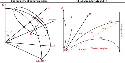
Left: the geometry of pulsar emission (Zhang et al. 2007). Ω and μ are the rotation axis and the magnetic axis. ζ, α, β = ζ − α and θμ are the angle of the observer's line of sight relative to the rotation axis, the magnetic inclination angle, the impact angle and the angle of radiation direction to the magnetic axis, respectively. ϕ represents the azimuth angle around the rotation axis and ψ is the angle between the magnetic field plane and the Ω–μ plane. C is the point at which we observe radiation when the line of sight sweeps the emission beam from A to B. Right: a simple diagram for the AG and the CG in the magnetosphere of a neutron star (NS) (Qiao et al. 2007). NCS represents the null change surface where Ω · B = 0. CFL and LOF denote the critical field line and the last open field line, respectively.
The simulated results of the ICS model are shown in Fig. 5 (PSR B0329+54) and Fig. 6 (PSR B1642−03), where the red and blue solid/dashed lines represent the observed waves going out from points A and A΄, respectively (see Fig. 7). Figs 5(a) and 6(a) present the beaming angle evolution in relation to radiation frequency, whereas Figs 5(b) and 6(b) show the evolution of the radiation altitude in relation to the radiation frequency. Using the ICS model to simulate the evolution of the radiation altitude and beaming angle versus radiation frequency, we obtained the parameter values of γ0 ∼ 2 × 10⁵ and k ∼ 0.329 for PSR B0329+54, and γ0 ∼ 1.6 × 10³ and k ∼ −0.02 for PSR B1642−03. Meanwhile, the field lines where the radiation comes from and the sparking points A and A΄ are also determined by the simulation. The foots of the field lines above the polar cap are located at 0.98 Rp for PSR B0329+54 and 0.46 Rp for PSR B1642−03. The locations of the sparking points above the polar cap are 0.98 Rp for PSR B0329+54 and 0.46 Rp for PSR B1642−03, where Rp = R1.5Ω0.5c−0.5 represents the polar cap radius defined by the foot of LOF; here, R, Ω and c are the pulsar radius, rotation angular velocity and light speed, respectively (Ruderman & Sutherland 1975). In Figs 5 and 6, the theoretical curve of the ICS model shows a down–up–downward trend, which is consistent with the conclusion of Qiao & Lin (1998); Zhang et al. (2007). For each profile, the radiation altitudes of the inner cone components are lower than those of the outer cone components. The radiation altitudes of the outer components decrease as the radiation frequency increases, whereas the radiation altitudes of inner cone components increase as the observing frequency increases.
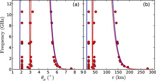
Simulated results of the beam–frequency evolution of PSR B0329+54 in the ICS model. Panels (a) and (b) present the evolution of the beaming angle θμ and the emission altitudes versus frequency, respectively. The red dots correspond to emission altitudes. The blue and red solid lines correspond to ICS fitting curves. The values of γ0 and k are set to 2 × 10⁵ and 0.329, respectively.
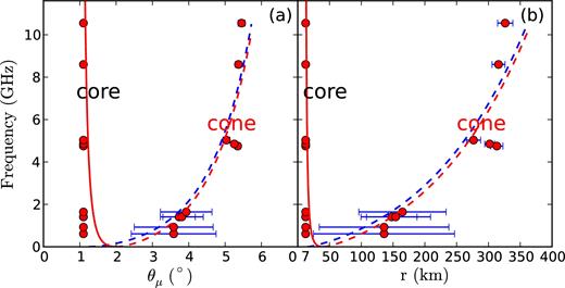
As for Fig. 5, but for PSR B1642−03 with γ0 = 1.6 × 10³ and k = −0.02. The fitting curves are plotted with solid curves for the core component and dashed curves for the cone component.
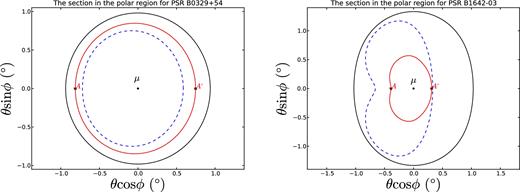
The black solid and blue dashed lines are the LOF and CFL, respectively. The region between the blue dashed line and the black solid line is the AG and the region surrounded by the blue dashed line is the CG. The red solid line is the magnetic field line where the radiation comes from. The red solid line is also the section of all the sparking points in the AG or the CG. The red star dots A and A΄ are the sparking points used in our calculation. For PSRs B0329+54 and B1642−03, the values of α are 30|$_{.}^{\circ}$|0 and 68|$_{.}^{\circ}$|2, respectively.
3.3 Radiation region
In an oblique rotator with a dipolar magnetic field, the shapes of the CG and the AG are a function of the pulsar period and inclination angle α (Qiao et al. 2004; Wang et al. 2006; Lee et al. 2006a). The CG and AG in the open magnetic field region are shown in Fig. 4. Qiao et al. (2004) point out that sparking may take place in these two gaps, which will lead to pair production and generate secondary particles. These particles would be accelerated in the CG or AG to produce radiation through the ICS process. The radiation region of the pulsar can be determined conclusively if the sparking point and the magnetic field line where the radiation comes from are determined; detailed calculation methods are given by Qiao et al. (2004), Wang et al. (2006) and Lee et al. (2006a).
We try to determine the radio radiation regions of PSRs B0329+54 and B1642−03 by using the simulated results in Section 3.2. The shapes and widths of the radiation regions above the polar cap are shown in Fig. 7. For PSR B0329+54, the section of the foots of the field lines where the radiation comes from (denoted by the red solid line) and the sparking points A and A΄ above the polar cap are located at the region between those of the LOF (black solid line) and the CFL (blue dashed line). We have also obtained a simulation of beam–frequency, although the simulation is not optimal considering the fact that the radiation was generated from the CG. Therefore, the CG and AG can be responsible for the radiation of PSR B0329+54. For PSR B1642−03, however, the section of the foots of the field lines where the radiation comes from (red solid line) and the sparking points above the polar cap are located at the region surrounded by the CFL, which means that the radiation of PSR B1642−03 is generated mainly from the CG.
4 DISCUSSION AND CONCLUSIONS
With the multi-Gaussian function, we separated the radiation components of the multiband radio pulse profiles of PSRs B0329+54 and B1642−03, and calculated the radiation altitude of each radiation component (r = 20–280 km for PSR B0329+54 and r = 10–330 km for PSR B1642−03). Then, we conducted further simulations over the evolutions of radiation altitudes and beaming angles using the ICS model, as well as obtaining the Lorenz factors (γ0 ≃ 105 for PSR B0329+54 and γ0 ≃ 103 for PSR B1642−03) and the energy loss factors of high-energy particles (k = 0.329 for PSR B0329+54 and k = −0.02 for PSR B1642−03). Finally, we received the radio radiation regions of the two sources.
It is suspected that the radio emission beam of pulsars may include core and multicone components (Rankin 1983, 1993; Lyne & Manchester 1988; Wu et al. 1992, 1998; Manchester 1995; Zhang et al. 2007). Now, the pulse profiles of PSRs B0329+54 and B1642−03 show obvious multipeak characteristics, which can be described by multi-Gaussian functions (five Gaussians for PSR B0329+54 and three Gaussians for PSR B1642−03; see Figs 1 and 2 for details), which supports the scenario of core and cone components. However, the formation and radiation mechanisms of multicomponents are still disputable. We find that the multicomponents of the two sources can be described well by the ICS model, which implies that the core and cone components may be generated by the same radiation mechanism. This is consistent with the conclusion of Lyne & Manchester (1988).
In most cases, the integrated pulse profiles of pulsars are extremely stable. However, in the case of a moding pulsar (Backer 1970; Helfand, Manchester & Taylor 1975; Wang, Manchester & Johnston 2007; Kijak et al. 1998; van Leeuwen et al. 2002; Redman, Wright & Rankin 2005), during an observation, if a mode change occurs, the observed profile will be different from the profile of any individual mode. Furthermore, when moding occurs, the observed pulse profile will no longer be stable because the relative contribution of each mode is different. For PSR 0329+54, a mode change of the pulse profile was observed (Lyne, Smith & Graham 1971; Bartel et al. 1982; Hesse, Sieber & Wielebinski 1973; Izvekova et al. 1994; Kuz'min & Izvekova 1996; Suleimanova & Pugachev 2002; Chen et al. 2011). Does this change of mode influence our results? For PSR 0329+54, Kuz'min & Izvekova (1996) found that: ‘[w]hen the mode changes, the component structure (the number of the components and their positions in phase) does not change; only the relative intensity of the components varies.’ We also come to the same conclusion by analysing some mode changing data of PSR B0329+54. Therefore, the mode switching phenomenon does not influence our result. In the future, we plan to use large-aperture telescopes (e.g. the five-hundred-meter aperture spherical radio telescope, FAST) for long-term monitoring of pulsars such as PSRs B0329+54 and B1642−03. We also plan to study the evolution of pulse profiles with the new data and the ICS model in order to verify the conclusions presented in this paper.
It is very important to determine the radiation locations by analysing the observed multifrequency pulse profiles in order to understand how the radiation is generated in the pulsar magnetosphere and in order to constrain pulsar radiation models. For PSRs B0329+54 and B1642−03, the sparking and related radiation can take place in both the CG and AG. Can we observe the radiation of these two pulsars from both the CG and AG? The answer depends on the inclination angle α and the impact angle β (or viewing angle ζ = α + β). From the observed values of α and β (Lyne & Manchester 1988; Rankin 1993), under the dipole magnetic field assumption, radiation regions are calculated geometrically. It was found that either the CG or the AG can be responsible for the radio radiation of PSR B0329+54, whereas the radiation is likely to be generated just in the CG for PSR B1642−03. Besides the particle acceleration and radiation locations, another question is what shapes of pulse profiles can be observed. The shapes of pulse profiles change with different frequencies. The beam–frequency evolution presents a constraint to all theoretical models. The ICS model has two typical beam–frequency maps – the observing frequency is plotted versus the beaming angle or altitudes of radiation points (Qiao & Lin 1998; Qiao et al. 2001). The beam–frequency maps of PSRs B0329+54 and B1642−03 (Figs 5 and 6 in this paper) show these two types, respectively. Of particular note, the beam–frequency map of PSR B1642−03 shows that the pulse profiles become wider at higher frequencies, which challenges other theoretical models.
The Lorentz factors we used for simulating the observed data are ∼105 for PSR B0329+54 and ∼103 for PSR B1642−03 (see Figs 5 and 6). These Lorentz factors are larger than those (γ ≃ 800) of secondary particles and lower than the energy of the primary particles γ0 ≃ 106 given by Ruderman & Sutherland (1975). In the CR model (Ruderman & Sutherland 1975), pair production needs Lorentz factors of primary particles as large as 106. As discussed by Zhang et al. (2007), not all pairs are produced at the bottom of the gap, and therefore not all primary particles can gain such a large Lorentz factor. When the pairs are generated outside the gap, the Lorentz factor will be ≲106. This means that the Lorenz factor γ0 used in this paper is reasonable.
Acknowledgments
This work was supported by the Strategic Priority Research Programme of the Chinese Academy of Sciences (Grant No XDB23000000), the National Natural Science Foundation of China (Grant Nos 11565010, 11373011, 11225314, 11033008, 11165005, 11173046, 11403073, 11303069 and 11173041), the Science and Technology Innovation Talent Team (Grant No (2015)4015), the Training Programme for Excellent Young Talents (Grant No 2011-29), the High Level Creative Talents (Grant No (2016)-4008) and the Innovation Team Foundation of the Education Department (Grant No [2014]35) of Guizhou Province, the Natural Science Foundation of Shanghai No 13ZR1464500, the Scientific Programme of Shanghai Municipality (08DZ1160100), the Knowledge Innovation Programme of CAS (Grant No KJCX1-YW-18), the Strategic Priority Research Programme, the Emergence of Cosmological Structures of CAS (Grant No XDB09000000), the Doctoral Starting Up Foundation of Guizhou Normal University 2014, the Science and Technology Foundation of Guizhou Province (Grant Nos J[2015]2113 and LH[2016]7226) and the Postgraduate Innovation Foundation of Guizhou Normal University (Grant No 201527). DL and QJZ are members of the CAS Interdisciplinary Innovation Team. This work is also supported partially by the fund of the ‘Special Demonstration of Space Science’ and by the strategic Priority Research Programme of CAS (Grant No XDB23010200).
We would like to thank the Yunnan Astronomical Observatory (CAS), the Shanghai Astronomical Observatory (CAS) and the European Pulsar Network data base for providing observation conditions and valuable data resources.
REFERENCES
