


Abstract
In this work, we use the semi-empirical atmospheric modelling method to obtain the chromospheric temperature, pressure, density and magnetic field distribution versus height in the K2 primary component of the RS CVn binary system HR 7428. While temperature, pressure and density are the standard output of the semi-empirical modelling technique, the chromospheric magnetic field estimation versus height comes from considering the possibility of not imposing hydrostatic equilibrium in the semi-empirical computation. The stability of the best non-hydrostatic equilibrium model implies the presence of an additive (towards the centre of the star) pressure that decreases in strength from the base of the chromosphere towards the outer layers. Interpreting the additive pressure as magnetic pressure, we estimated a magnetic field intensity of about 500 G at the base of the chromosphere.
1 INTRODUCTION
HR 7428 (=V 1817 Cygni) is a bright (V = 6.3) long-period (108.578 d) spectroscopic RS CVn binary composed by a K2 II–III star and a main-sequence A2 star (Parsons & Ake 1987). The magnetic activity of the system is well known: Ca ii H & K emission was first reported by Gratton (1950), by a detailed analysis of photometric observations. Hall et al. (1990) were able to detect starspot signatures on the K2 primary star. It is now well established that the stellar atmosphere of cool stars is characterized by that temperature gradient inversion. An inversion is explained in the framework of the magnetic activity theories, but not yet definitively understood.
Late-type stars, with H α in emission, show also a fairly stable chromospheric emission outside flares; see e.g. Byrne et al. (1998). This reinforces the hypothesis that chromospheres are globally in a quasi-stationary state, modulated mainly by the stellar activity cycle, whose temperature–density structure results from the balance between global dissipation of non-radiative energy and radiative cooling (Kalkofen, Ulmschneider & Avrett 1999).
Most of what we know about stars and systems of stars is derived from an analysis of their radiation and this knowledge will be secure only as long as the analytical technique is physically reliable. A well-tested technique to get information on physical properties of chromospheric layers of active stars is the Non-Local-Thermodynamic-Equilibrium (NLTE) radiative transfer semi-empirical modelling: for different temperature versus height distributions, the NLTE populations for hydrogen are computed by solving simultaneously the equations of hydrostatic equilibrium, radiative transfer and statistical equilibrium. The emerging profiles for some chromospheric lines and continua are computed and compared to the observations. Then, the modelling is iterated until a satisfactory match is found (see e.g. Vernazza, Avrett & Loeser 1981; Fontenla, Avrett & Loeser 1993). These models are built to match the observations in different spectral features, and make no assumption about the physical processes responsible for the heating of the chromosphere, but can be used as constraints for these processes. The obtained models describe the variations of the essential physical parameters, in particular the temperature, pressure and electron density across the outer atmosphere, and give information on its ‘mean’ state, both temporally and spatially.
The most important problem of this approach lies in the uniqueness of the solution. In fact, knowing that a particular atmosphere would emit a line profile like the one we observe for a given star does not imply that the star has indeed this atmospheric structure, since we do not know whether some other atmosphere would produce the same profile. To solve, or at least to reduce, this problem, the modelling has to be based on several spectral features, with different regions of formation. The amount and the kind of diagnostics used to build an atmospheric model are in fact very important; by combining several spectral lines that are formed at different but overlapping depths in the atmosphere, we can obtain a more reliable model (Mauas, Cacciari & Pasquini 2006).
Certainly the best known semi-empirical model is the one for the average Quiet-Sun, Model C by Vernazza et al. (1981). Semi-empirical modelling was successfully applied also to the atmospheres of cool stars. An extensive modelling of dM stars has been done starting with the work by Cram & Mullan (1979), Short & Doyle (1998), Mauas & Falchi (1994) and Mauas et al. (1997). Furthermore, a rich history of semi-empirical chromospheric modelling has been also carried out for cool giant and supergiant stars (see e.g. Kelch et al. 1978; Basri, Linsky & Eriksson 1981; Luttermoser, Johnson & Eaton 1994). In cool stars, the application of NLTE semi-empirical chromospheric modelling can be based on optical and ultraviolet (UV) observations. This is because lines such as the H α Na i D Ca ii IRT become dominated by electron-collision excitation processes, which make them effective chromospheric diagnostics (Houdebine 1996). The possibility of using H α profile as a diagnostic of stellar chromospheres was discussed in detail by Cram & Mullan (1979) and Mullan & Cram (1982) in terms of control of the source function by photons or collisional processes. H α is observed in active stars in a wide variety of shapes and sizes; when the effective temperature is low enough, the collisional control of the H α source function becomes possible over a wide range of chromospheric pressures, and, under these conditions, H α can be a good chromospheric diagnostic. Mg ii H & K UV lines, due to their large opacity, provide excellent diagnostic over a wide range of heights of the outer chromospheric layers (Uitenbroek 1992), and Ca ii IRT triplet is a constraint for the shape of the middle chromosphere from the temperature minimum up to the plateau (Andretta et al. 2005).
Here, we applied the NLTE semi-empirical chromospheric modelling to the K2 star of HR 7428 binary system basing the analysis on the H α, H β, Na i D, Ca ii IRT triplet, Mg ii H & K lines and UV continuum diagnostics.
2 DATA ACQUISITION AND REDUCTION
H α Na i D H β Ca ii IRT spectroscopic observations of HR 7428 were carried out at the 91-cm telescope of Catania Astrophysical Observatory, ‘M. G. Fracastoro’ station (Serra La Nave, Mt Etna, Italy), using the new Catania Astrophysical Observatory Spectropolarimeter (CAOS), which is a fibre-fed, high-resolution, cross-dispersed echelle spectrograph (Spanó et al. 2004, 2006; Leone et al. 2016).
The spectra were obtained in 2015 September. Exposure times have been tuned in order to obtain a signal-to-noise ratio of at least 200 in the continuum in the 390–900 nm spectral range, with a resolution of |$R=\frac{\lambda }{\Delta (\lambda )}$| = 45 000, as measured from ThAr and telluric lines.
Echelle iraf packages have been used for data reduction, following the standard steps: bias subtraction, background subtraction, trimming, flat-fielding and scattered light subtraction, extraction for the orders and wavelength calibration. Several thorium lamp exposures were obtained during each night and then used to provide a wavelength calibration of the observations. Each spectral order was normalized by a polynomial fit to the local continuum. A reduced spectrum, in the wavelength ranges of the line of interest, is shown in Fig. 1. In the plotted spectrum, the average S/N obtained at the continuum close to H α is about 200.
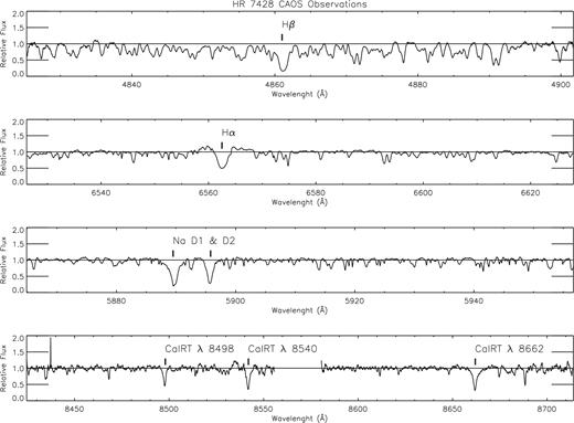
HR7428 normalized spectrum obtained using the new CAOS showing the line profiles of H β, Na i D, H α and Ca ii IRT lines.
Mg ii H & K spectroscopic observations have been obtained in 1997 by the IUE satellite. The IUE spectra have been corrected for interstellar extinction. According to the Hipparcos, distance d = 323±52 pc and to the typical value of 1 mag per kpc for interstellar extinction we adopted for the computation A(V) = 0.32. Assuming the standard reddening law A(V) = 3.1 × E(B−V), a colour excess E(B−V) = 0.10 has been derived. IUE spectra have been de-reddened according to the selective extinction function of Cardelli, Clayton & Mathis (1989).
The spectral resolution is about 0.2 Å for the Mg ii region. The IUE flux calibrated HR7428 spectrum is shown in Fig. 2.
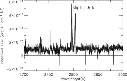
HR7428 high-resolution flux calibrated spectrum in the wavelength of the Mg ii line profile obtained by International Ultraviolet Explorer (IUE).
Unfortunately, we have no simultaneous UV and optical observations. Therefore, we have to take into account the activity variability that could affect the HR7428 system, due to different levels of the stellar activity and/or different distribution of the active regions on the visible surface, in different times. In order to have an estimate of how much UV data are affected by activity variability, we have compared two IUE spectra of the system, obtained in different dates: LWP26775HL.FITS obtained in 1997 November and LWR10313HL.FITS obtained in 1995 December (see Fig. 3, where the two Mg ii H & K IUE spectra are shown with a shift in wavelength in order to overlap) 1.060 × 10⁻¹² ± 1 × 10⁻¹⁵. We find that we can neglect the long-term variability as far as the UV continuum is concerned, the two spectra show in fact the same continuum mean value (Mg ii Continuum Flux (1995) = 1.06 × 10⁻¹² ± 1 × 10⁻¹⁴ erg cm−2 s−1, Mg ii Continuum Flux (1997) = 1.060 × 10⁻¹² ± 7 × 10⁻¹⁵ erg cm−2 s−1). As far as the Mg ii H & K line profiles are concerned, we measure approximately equivalent observed fluxes at Earth (FluxMg ii H & K (1995) = 3.33 × 10⁻¹¹ ± 3 × 10⁻¹³ erg cm−2 s−1, Mg ii H & K (1997) = 3.20 × 10⁻¹¹ ± 3 × 10⁻¹³ erg cm−2 s−1), but the profile shape is quite different as shown in Fig. 3, most probably indicating a different distribution of active regions in different times that we cannot take into account. Therefore, a higher weight will be done to the best fit of the UV continuum with respect to the Mg ii H & K line profile.
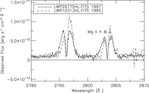
Comparison of two IUE spectra of the system, obtained in different dates: LWP26775HL.FITS obtained in 1997 November and LWR10313HL.FITS obtained in 1995 December.
3 COMPUTATIONAL METHOD
Historically, K2 giants were classified as ‘non-coronal’ stars; however, in the late 1990s, evidence for transition region emission was detected for Arcturus (K2 III) and Aldebaran (K5 III) (Ayres, Brown & Harper 2003) and for other representative ‘non-coronal’ red giants (see e.g. Ayres et al. 1997; Robinson, Carpenter & Brown 1998). Therefore, here, the atmospheric model of the K2 primary magnetic active component has been built computing a photospheric model, a chromospheric model and a transition region model and joining the three together; we assume a plane-parallel geometry in our modelling efforts.
3.1 Photospheric model
Taking into account the Marino et al. (2001) physical parameters (see Table 1), we selected from the Castelli LTE synthetic spectra data base (http://www.oact.inaf.it/castelli/castelli/grids.html), a spectrum with parameters log g ≅ 2.0, |$T\rm _{eff}\cong$| 4400 K and solar metallicity that describes the photospheric contribution of the K2 primary component, and a spectrum with parameters log g ≅ 4.0, |$T\rm _{eff}\cong $| 9000 K, and solar metallicity that describes the flux contribution of the A2 secondary component of the binary system HR 7428.
In Fig. 4, the fluxes at Earth of the two LTE models are shown together with their sum. The original fluxes have been converted to flux at Earth by the conversion factor R2/d2, which has been calculated for the K and A stars according to the parameters given in Table 1. From the plot we conclude that, for NLTE radiative transfer calculations of the H β, Na i D, H α, Ca ii IRT triplet profiles of the binary system, we can neglect the A2 star contribution. In fact, from Fig. 4, we can see that for wavelength longer than 3200 Å, the continuum flux of the binary system is dominated by the K star. This is in agreement with Marino et al. (2001), who find that the A2 star contribution to the total flux in the H α region is only 4 per cent. On the other hand, in order to calculate the NLTE Mg ii H & K (wavelength lower than 3200 Å) HR 7428 line profile, we have to take into account the A2 star contribution. In the Mg ii H & K spectral range in fact (triangles show the observed IUE Mg ii H & K), the observed continuum is dominated by the A star contribution.
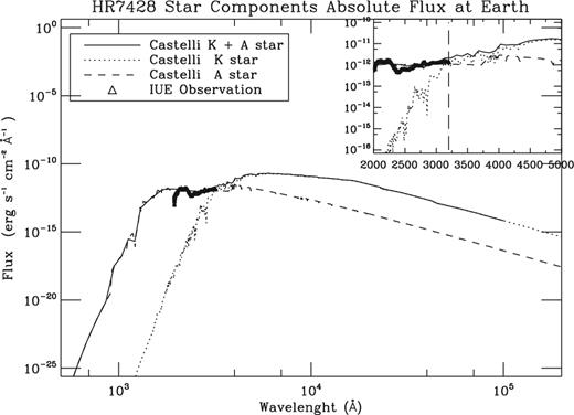
HR7428 Castelli LTE synthetic photospheric fluxes at Earth for the K star (dotted line) and A star (dashed line) where the conversion factor R2/d2 has been calculated for the K and A stars according to the parameters given in Table 1. The plot zoom around 2000–5000 |$\mathring{\rm A}$| shows that before λ = 3200 |$\mathring{\rm A}$| the A star dominates the continuum emission, while for wavelength greater than λ = 3200 |$\mathring{\rm A}$| we can neglect the A star contribution, the continuum is in fact dominated by the K star.
HR 7428 K2II–III and A2 components (Marino et al. 2001).
| Element | Primary (cooler K2II-III) | Secondary (hotter A2) |
|---|---|---|
| R | 40.0 ± 6.5R⊙ | 2.25 ± 0.5R⊙ |
| |$T\rm _{eff}$| | 4400 K ± 150 K | 9000 K ± 200 K |
| log g | 2.0 ± 0.5 | 4.0 ± 0.5 |
| Element | Primary (cooler K2II-III) | Secondary (hotter A2) |
|---|---|---|
| R | 40.0 ± 6.5R⊙ | 2.25 ± 0.5R⊙ |
| |$T\rm _{eff}$| | 4400 K ± 150 K | 9000 K ± 200 K |
| log g | 2.0 ± 0.5 | 4.0 ± 0.5 |
Therefore, we computed the A2 secondary component atmospheric model by the atlas9 code (Kurucz 1993) using the parameters log g = 4.0, |$T\rm _{eff}$| = 9000 K, [A/H] = 0.0.
The atmospheric model of the K2 primary magnetic active component has been built computing separately a photospheric model, a chromospheric model and a transition region model and joining the three together.
The K2 photospheric model was computed using the atlas9 code and the parameters log g=2.0, |$T\rm _{eff}$|= 4400 K, [A/H]=0.0 for the K2 primary component.
3.2 Transition region model
A first estimation of a plane-parallel model for the lower transition region of the HR 7428 K2 primary component has been built using the method of the volumetric emission measure. The use of emission measure techniques to construct transition region models is well established (see e.g. Jordan & Brown 1981; Harper 1992); the flux at the star, for lines forming at temperature Te ≈ 105 K, is in fact dominated by collisions. This results in emission lines that are optically thin and with a contribution function sharply picked in temperature, that is, typically formed over a temperature range of Δlog (Te) = 0.30.
The above conditions allow us to determine the temperature gradient as a function of the averaged emission measure over Δlog (Te) = 0.30, which we indicate as EM0.3.
By imposing hydrostatic equilibrium, including turbulent pressure, the transition region model can be obtained combining the temperature gradient as a function of EM0.3 and the pressure variation from the equation of hydrostatic equilibrium (see e.g. Harper 1992).
We used the equations above in order to build plane-parallel models for the lower transition region of the HR 7428 K2 primary component.
In order to have an estimate of emission measures for the HR 7428 binary system, we used the values of volumetric emission measure (VEM) versus |$T\rm _{eff}$| measured by Griffiths & Jordan (1998) for another RS CVn system, HR 1099 primary component (RHR1099 K1IV = 3.9 R⊙), opportunely scaling them, in order to take into account the bigger radius (RK2 = 40 R⊙) of HR 7428 K2 star, according to the formula EM0.3 = VEM/4πR2 (Brown et al. 1991) and the parameters of Table 1.
From the estimated EM0.3 values, a grid of 161 transition region models, shown in Fig. 5, has been built by means of equations (1) and (2) using a grid of 23 values of electron density at the fixed temperature Te = 50 000 K obtained scaling of a factor from 0.5 up to 30 the values of electron density at 50 000 K measured in HR 1099 (Ne = 5 × 10+11cm−3). For each of these 23 electron density values, a grid of seven values of the turbulent velocity in the layer with T0 = 104 K, vturb(T0 ≡ 104K) = 10, 20, 30, 40, 50, 60 and 70 km s−1 has been considered for the calculation of turbulent velocity distribution according to the empirical law by Griffiths & Jordan (1998) vturb(T) = vturb(T0) × (T/T0)1/4 between log (T) = 4.0 and log (T) = 5.3.
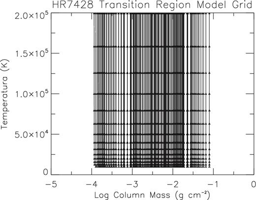
Grid of transition region models used for the study of HR7428 atmosphere. The grid has been built as described in the text.
These transition region models provide the upper boundaries for the radiative transfer calculations of the chromospheric models, while the adopted photospheric model provides the lower boundaries of the chromospheric models.
3.3 Chromospheric model
The term ‘chromosphere’ indicates the region above a stellar photosphere where non-radiative heating processes (either magnetic or acoustic) become important in the energy balance and where hydrogen is partially ionized. Since hydrogen is nearly completely ionized when temperatures reach 20 000–30 000 K, we consider this the top of chromosphere. Once hydrogen is nearly completely ionized, mechanical heating produces a steep thermal gradient because there is no cooling channel as effective as hydrogen, and Ca ii , Mg ii have disappeared before hydrogen is ionized (Linsky et al. 2001).
Chromospheres lies in the difficult regimes of non-LTE and non-ionization equilibrium. While photosphere can be calculated in detail when having log g, [A/H] and |$T\rm _{eff}$|, and transition region can be constrained by observations because lines form in optically thin conditions as seen before, for the chromospheric layers we have no constraints, lines are optically thick and the chromospheric model has to be based upon spectral diagnostic methods by means of semi-empirical modelling technique, that is changing a hypothetic model iteratively, in order to match as many as possible observations that form in the chromospheric layers. We can only suppose that the temperature increases with a smooth thermal gradient because the non-radiative sources heat the plasma producing bright emission in the H α, Ca ii IRT, Mg ii H & K, which together are the dominant cooling channels of the chromosphere. In Sun, the chromosphere goes from ≈600 km and ≈2000 km above the photosphere and is characterized by temperature gradient sign change, where temperature smoothly grows from ≈4500 K up to ≈15 000 K over which the gas density changes by several orders of magnitude due to a sharp decrease of turbulent pressure while the electron density only smoothly decreases.
The solar chromosphere has been described for the first time by Vernazza, Avrett & Loeser (1973) by means of a one-component model of the solar atmosphere, including in that model the photosphere, chromosphere and transition zone, and then, in detail, by Fontenla et al. (1999), who, using the pandora NLTE radiative transfer code, determine semi-empirical models for seven semi-empirical models for sunspots, plages, network and quiet atmosphere constructed to reproduce observed emergent intensities and profiles at wavelengths from the UV to radio wavelengths.
While Vernazza et al. (1973) determine the chromospheric model of Sun by adjusting the temperature as a function of height to that distribution that gives best agreement between synthesized and observed line spectra, here we have built a wide grid of chromospheric models from which to look for the best model by means of a χ2 minimization selection method.
In particular, for each one of the 161 transition region model and for each of nine values of Tmin in the range between ∼2800 K and 4200 K that we have chosen with a step of less than 200 K as points where to cut the photospheric Kurucz model, a grid of 25 chromospheric models is generated by a smooth spline interpolation between the photosphere and the transition region using as free parameters a grid of 5 × 5 interpolation knots (see Fig. 6, where the grid of 25 chromospheric models is shown for a fixed TR model and a fixed minimum of photospheric model Tmin). We impose the chromospheric structures to have a monotonic temperature dependence on column mass (dT/dm ≤ 0). Fig. 6 shows how the temperature gradient constraint strongly cuts the number of useful model of the grid, for example in the 25 model grid of the figure, only eight models satisfy the gradient constraint and can be used in the analysis.
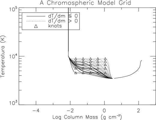
Grid of chromospheric structures obtained by spline interpolation between a fixed transition region model and a fixed photospheric model, using as free parameters a grid of 25 knots point. The figure shows in dotted lines the models that do not satisfy the negative gradient condition dT/dm ≤ 0.
The total grid of models includes 161 × 9 × 25 = 36 225 models, and only 15 691 satisfy the dT/dm ≤ 0 constraint and have been considered in the NLTE radiative transfer.
3.4 Computation: applying or not hydrostatic equilibrium equations
The coupled equations of radiative transfer and statistical equilibrium were solved using the version 2.2 of the code multi (Carlsson 1986), for the H, Ca, Na, Mg atomic models. The H atomic model incorporates 16 states of H, with 84 b–b and 9 b–f transitions. The Ca atomic model incorporates eight states of Ca i, the lowest five states of Ca ii and the ground state of Ca iii, 9 b–b and 13 b–f transitions are treated in detail. The Mg ii atomic model is made of three states Mg i, the lowest six states of Mg iiand the ground state of Mg iii, nine b–b and nine b–f transitions are treated in detail. The Na atomic model incorporates 12 levels: 11 levels of Na i and the ground state of Na ii and 29 b–b and 11 b–f transitions are treated in detail. The opacity package included in the code takes into account free–free opacity, Rayleigh scattering and bound–free transitions from hydrogen and metals. We include the line blanketing contribution to the opacity using the method described in Busá et al. (2001).
As a first step, we imposed hydrostatic equilibrium to the hydrogen, that is, we calculated the hydrogen radiative transfer and the equation of hydrostatic equilibrium consistently. In detail, starting with the LTE hydrogen populations for the electron pressure and density calculation, hydrogen is iterated to convergence. Then, hydrostatic equilibrium dPTot = ρg dh is solved and electron pressure and hydrogen populations are updated, the loop continues until we obtain a convergence. The electron density obtained is then used to solve the Ca, Mg and Na radiative transfer and statistical equilibrium equations. The population densities obtained from the H calculation are used to obtain the background NLTE source function in the Ca, Mg and Na calculations. This computation modifies the initial grid because a new column of electron density is obtained, we find that only 2052 models converge to a solution and we call them HSE models.
We also considered not imposing hydrostatic equilibrium that means fixing the electron densities to the ones of the original grid. In this case, we consider all the 15 691 models that only satisfy the dT/dm ≤ 0 constraint and we call these models NOHSE models.
Even if an atmospheric model in non-hydrostatic equilibrium is not realistic and should be rejected, here we assume the NOHSE models as good as the HSE ones. Of course, hydrostatic equilibrium has to happen in the star, but, because we are not taking into account all the pressure contributions to the total pressure, therefore we can assure that also the HSE models should be rejected, or, at least can be, good or not, just like the NOHSE models. In a sense, we can assume that, imposing HSE, the resulting model is not in hydrostatic equilibrium if a contribution to the pressure is missing in the dPTot = ρg dh equation. And this is the case of cool active stars. We know in fact that the atmospheres of active stars are permeated by magnetic fields that emerge from deeper layers. With increasing height, we might expect the structure to be more greatly influenced by magnetic fields, since the energy density of the magnetic fields should fall off more slowly than the energy density of the gas (this is the case of solar atmosphere where β = 8πNKTe/|(B)|2 is ≥1 in photosphere and <<1 in transition region layers). Therefore, magnetic pressure should be added in the computation of the total pressure and is not. This lack, together with the lack of any other possible contribution, is not yet identified; let us say that the electron densities and the hydrogen populations obtained from imposing HSE differ from the ones we would have obtained introducing a magnetic field contribution. This approach takes into account the possibility that some pressure contributions are neglected and become a method to derive an estimate of the lacking pressure component. In such an approach, we use the electron density as a free parameter, looking for the electron density distribution that best fit the data. We accept as best solution, also a distribution whose total pressure is not balancing the gravity, accepting the hypothesis that a new pressure component could be considered for achieving the equilibrium.
Furthermore, also different approaches in the treatment of line blanketing produce different Ne versus temperature. It is well known in fact that the source function of a line can be strongly coupled to radiation fields even at very different wavelengths, via radiative rates determining the statistical equilibrium of the species producing the line.
If we would find as the best model reproducing our data, an HSE model, this would mean that magnetic or other contributions to the total pressure are negligible in the whole upper atmosphere of the K2 HR 7428 star.
In the case where a NOHSE model should best reproduce the observations, this would imply that other pressure contributions are important in the outer atmosphere of our star and we can then infer information on these additive contributions to the total pressure.
Therefore, both the HSE grid of 2052 models and the initial grid of 15 691 model have been considered in the radiative transfer calculations for H, Na, Ca and Mg. For each grid, the models that converge to solution for all the atoms have been taken into account for the comparison with the observed spectrum.
The computed profiles of H α, H β, Ca ii IRT, Na i D, have been convolved with a rotational profile with v sin i = 17 km s−1 (Marino et al. 2001) and an instrumental profile with R = |$\frac{\lambda }{\Delta (\lambda )}$| = 45 000, normalized and then compared with observations.
The computed profiles of Mg ii H & K have been obtained by the weighted sum of the K2 star profile and the A2 star profile and weighted for the d2/R2 factor. Wavelength shifts to account for orbital velocities are applied to synthetic spectra.
4 COMPARISON WITH OBSERVATIONS: THE BEST MODEL
We used a χ2 minimization procedure for the selection of the model that best describes the mean outer atmosphere of HR 7428.
For each line, the χ2 between each observed and the synthetic line profile has been performed interpolating to the same wavelength grid the two profiles and choosing opportunely the wavelength range for the χ2 determination. Therefore, for each model, the whole set of observed lines has been compared with the corresponding synthetic lines and a global |$\chi ^2_{\text{Tot}}$| for each model has been calculated as the average of the χ2 obtained for the single line profiles, a 0.5 weight has been applied to the Mg ii H & K lines χ2 in order to take into account the activity-variability as shown in Section 2. We defined a selection box formed of those models that give a χ2 less than a fixed value for all used lines and UV continuum, the best model is than selected as the one of the box with the lowest |$\chi ^2_{\text{Tot}}$|.
We find that the best NOHSE model has a |$\chi ^2_{\text{Tot}}$| = 1.22 while the best HSE model has a |$\chi ^2_{\text{Tot}}$| = 2.60. This result lets conclude that the NOHSE best model distribution of temperature, gas pressure, electron and population densities versus height is the best description of the mean outer atmosphere of the K2 star of the binary system HR7428.
We will describe here both the two HSE and NOHSE best models as possible representations of the mean outer atmosphere of the K2 star.
The best |$\chi ^2_{\text{Tot}}$| of the NOHSE model with respect to the HSE one is clearly understable from Fig. 7, where the H α, H β, Ca ii IRT, Na i D synthetic profiles computed for the best HSE (dotted line) and the best NOHSE (dashed line) models are shown and compared with the observed profiles.
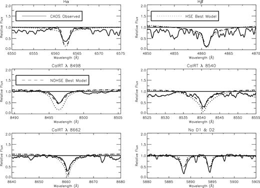
NLTE H α, H β, Ca ii IRT, Na i D normalized profiles computed for the best HSE (dotted line) and the best NOHSE (dashed line) models compared with observations.
The NOHSE model gives Na i D lines somewhat less deep than the observed profile and an H α profile a bit deeper than the observed one. Nevertheless, the NOHSE model reproduces much better than the HSE both the Ca ii IRT line profiles and the H β profile; furthermore, the HSE model also gives Na i D lines less deep and H α deeper than the observed one.
The NOHSE model gives also a better fit of the Mg ii H & K lines as can be seen from Fig. 8, where the IUE observed flux at Earth of the Mg ii H & K is compared with the synthetic profiles obtained from the HSE (dotted line) and the NOHSE (dashed line) best models. We can see how the NOHSE best model better reproduces both the continuum emission and the Mg ii H & K line profiles. The discrepancy in the peak region of the H and K profiles is compatible with the activity variability or also to the unresolved ISM absorption line that has not been taken into account in the synthetic lines computation.
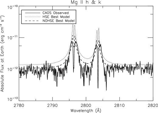
Mg ii H & K absolute flux profiles computed from the best HSE and the best NOHSE atmospheric models compared with the IUE observation.
Figs 9 and 10 show the line contribution functions (CF) to the emergent radiation (CF) as defined by Achmad, De Jager & Nieuwenhuijzen (1991), of the synthesized lines in the case of NOHSE and HSE, respectively. The plots mainly indicate the region of formation of the different part of each line, having on the x-axis the Δλ from the centre of the line and on the y-axis the column mass that corresponds to an atmospheric layer. In order to make this clearer, we overplotted the atmospheric model as a continuous line in each CF plot. In the case of Na i D, Mg ii H & K and Ca ii IRT, the CFs of the multiple lines are overplotted together.
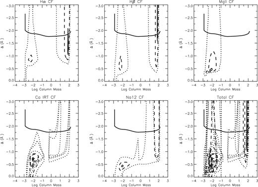
Contribution functions of the H α, H β, Mg ii H & K, Ca ii IRT, Na i D lines for the best NOHSE model. The maximum of the contribution function is set equal to 1. The contour plot indicates the fractions 0.9 (solid), 0.3 (dashed) and 0.01 (dotted). The atmospheric model is plotted as a solid line in each CF plot. The last plot, where all lines contribution functions are plotted together, indicates that our selected diagnostics mainly constraint the whole atmosphere from the photosphere (H α and H β wings), and chromosphere (all the lines) up to the transition region (Mg ii H & K cores) giving strength to our semi-empirical modelling.
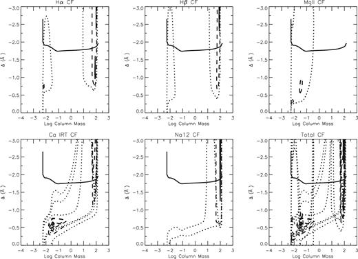
Contribution functions of the H α, H β, Mg ii H & K, Ca ii IRT, Na i D lines for the best HSE model. Like for the NOHSE model (see Fig. 9 also for the HSE model the outer atmosphere is enough constrained by our diagnostics).
We can see that both in the NOHSE and in the HSE atmospheres, the line formation is very similar.
We find that the base of the transition region is quite well constrained by the H α and Mg ii H & K cores. Also the central parts of the Na i D, H β and Ca ii IRT cores are affected by the transition region conditions. Mg ii H & K lines, except for the core, form entirely in the chromosphere, which is also constrained by the Ca ii IRT lines. The line wings of all the used lines, except for Mg ii H & K wings, form in the atmospheric region that goes from the photosphere up to the temperature minimum region. The last plot on the right in Figs 9 and 10 shows the overplot of all the lines CF and puts in evidence how the used diagnostics enough constrain the whole atmosphere, giving strength to the method and to the atmospheric model derived for the K2 star of HR 7428.
The HSE and NOHSE best models are shown in Fig. 11, compared with the Solar Val 3c model. We can see that the shape of both the HSE and NOHSE best models is quite similar to the Solar one. It is worthwhile to notice that the two models describe strongly different geometries. The HSE best model describes an atmosphere of the mean K2 primary component of the RS CVn system HR 7428 that extends up to 8 × 10⁵ km, the temperature decreases and reaches the minimum temperature of about 3000 K at about 500 000 km above the photosphere, the chromosphere extends for 250 000 km from the temperature minimum up to the base of the transition region that is located at about 800 000 km. The best NOHSE model is instead less extended of the HSE one; the temperature from the photosphere decreases, reaching the minimum of ≈3200 K at about 140 000 km above the photosphere, the chromosphere extends for 60 000 km from the temperature minimum up to the base of transition region that is located at about 200 000 km.
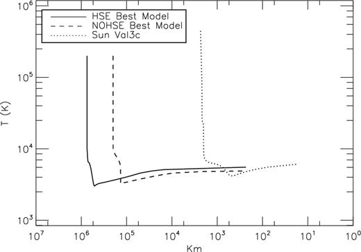
Best atmospheric HSE and NOHSE models for the mean K2 primary component of the RS CVn system HR 7428 compared with the Solar Val 3c model. The plot describes the distribution of temperature versus height. Height is given in kilometres measured above a zero-point where τ5000 = 1.
The difference between the HSE and the NOHSE models can be better understood from the plot of Fig. 12, where the temperature, electron density and total density are plotted versus column mass density (CM) defined as P/g for the best HSE and NOHSE models.
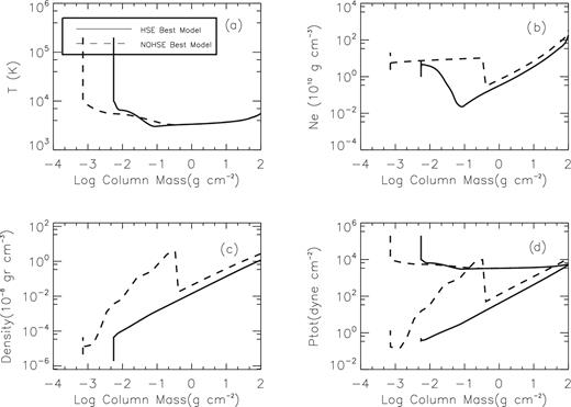
Temperature, electron density, density mass and pressure versus column mass for the best HSE and NOHSE models of the K2 primary component of the RS CVn system HR 7428. In the last plot, the two best models are shown for references.
From Fig. 12 panel a, we can see that the HSE best model has a minimum of temperature close to 3000 K when the log CM ≈−1.04 and a chromospheric ‘plateau’ at a temperature of about 6500 K at column mass ≈log CM = −2, then temperature rises up to 10 000 K and at log CM = −2.25, we find the base of transition region. In the transition region, the temperature rises abruptly up to 200 000 K while the column mass remains approximately constant. The NOHSE best model has a minimum of temperature ≈3250 K (250 K higher with respect to the HSE model) at a log CM ≈−0.48 a chromospheric plateau colder than the HSE one at about 5500 K and log CM = −2.1. The base of transition region is found here at log CM = −3.14 and then temperature rises abruptly up to 200 000 K while the column mass remains approximately constant. It is worthwhile to notice (panel b) that in the chromospheric region, the HSE model presents an electron density rising continuously, while in the NOHSE model, we observe an abrupt rise of the electron density in a few kilometres while in the main part of the chromosphere the electron density is approximately constant. This result is the same as that found from semi-empirical models of other cool stars (Harper 1992). This abrupt enhancement of electron density corresponds to a density enhancement and to an enhancement of the total pressure. Both in the HSE and in the NOHSE best models, in the chromospheric layers the density decreases uniformly up to the transition region. Here, both electron density and density decrease abruptly.
The most important difference between the two models is shown in Fig. 12 (panel d), where the total pressure is plotted versus column mass. While, in the HSE model, the total chromospheric pressure is imposed to be equal to the column mass multiplied for the gravity, that is PTot = CM × g, and we obtain a straight line, in the NOHSE model, the total chromospheric pressure exceeds the gravity pressure (dashed line is not a straight line but, in the chromospheric layers lays well above of the gravity pressure).
This exceeding pressure has to be balanced by an equal and opposite pressure, otherwise we cannot have a stable star. Therefore, we assumed the difference PTot − CM × g as equal, with opposite sign, to the lacking pressure in our calculations, that is: PTotnew = Pturb + Pgas + Pnew = CM × g and therefore Pnew = CM × g − PTot.
It is worthwhile to notice that not imposing hydrostatic equilibrium only refers to the chromospheric layers, both the used photospheric and transition regions models were calculated imposing hydrostatic equilibrium, therefore this new component pressure estimation refers only to this layer.
In Fig. 13, the new pressure component is shown in comparison to electron pressure, gas pressure, turbulent pressure. It is clear that this pressure component is not negligible being of the same order of strength of the gas pressure. In the hypothesis that the additive pressure could be a magnetic pressure, we calculated an ≈500 G magnetic field corresponding to a magnetic field that, from the base of the chromosphere, decreases towards the outer layers.
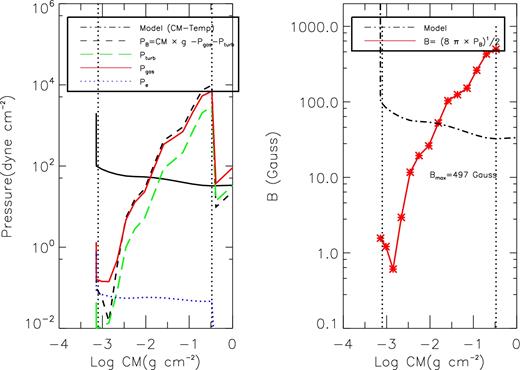
Left-hand panel: the new pressure component versus column mass is shown (dashed line) in comparison to electron pressure (blue), gas pressure (red) and turbulent pressure (green); the atmospheric model is overlapped (dot–dashed line) in order to identify the atmospheric layers where we are comparing the pressure components. Right-hand panel: magnetic field distribution versus column mass obtained considering the whole lacking pressure as magnetic pressure.
5 CONCLUSIONS
We present here the semi-empirical modelling for the K2 star of the RS CVn binary system HR 7428. The model has been computed to match a wide set of observations from the UV continuum to a set of chromospheric lines. The fine coverage in the parameter space used in the modelling made us able to find a good agreement between the observed and computed spectral features. Furthermore, a good agreement obtained in matching the UV continuum when use is made of the line-blanketing approximation method of Busá et al. (2001) reinforces the confidence on the method itself.
Although we have obtained an acceptable agreement between the calculations and the observations when the HSE is imposed, as it is usual, we do not find an HSE model that has a good match with all the used diagnostics. This could be due to many reasons; here we have explored the possibility that we are neglecting some components to the total pressure in the hydrostatic equilibrium equation. Therefore, we considered also the radiative transfers without imposing HSE. The best model in NOHSE gives a much better agreement with observations both in line profiles and in UV continuum.The stability of the best NOHSE model implies the presence of an additive (towards the centre of the star) pressure that decreases in strength from the base of the chromosphere towards the outer layers. Interpreting this additive pressure as a magnetic pressure, we estimated a magnetic field intensity of about 500 G at the base of the chromosphere.
Acknowledgments
We wish to thank the referee, Prof. Donald G. Luttermoser, for his careful reading of the manuscript and for his useful and kind comments and suggestions that we have greatly appreciated. iraf is distributed by the NOAO, which is operated by AURA under contract with NFS.
