


Abstract
We investigate possible signatures of halo assembly bias for spectroscopically selected galaxy groups from the Galaxy And Mass Assembly (GAMA) survey using weak lensing measurements from the spatially overlapping regions of the deeper, high-imaging-quality photometric Kilo-Degree Survey. We use GAMA groups with an apparent richness larger than 4 to identify samples with comparable mean host halo masses but with a different radial distribution of satellite galaxies, which is a proxy for the formation time of the haloes. We measure the weak lensing signal for groups with a steeper than average and with a shallower than average satellite distribution and find no sign of halo assembly bias, with the bias ratio of |$0.85^{+0.37}_{-0.25}$|, which is consistent with the Λ cold dark matter prediction. Our galaxy groups have typical masses of 1013 M⊙ h−1, naturally complementing previous studies of halo assembly bias on galaxy cluster scales.
1 INTRODUCTION
In the standard cold dark matter and cosmological constant dominated (Λ cold dark matter, CDM) cosmological framework, structure formation in the Universe is mainly driven by the dynamics of cold dark matter. The gravitational collapse of dark matter density fluctuations and their subsequent virialization leads to the formation of dark matter haloes from the highest density peaks in the initial Gaussian random density field (e.g. Mo, van den Bosch & White 2010, and the references therein). As dark matter haloes trace the underlying mass distribution, the halo bias (the relationship between the spatial distribution of dark matter haloes and the underlying dark matter density field) is naively expected to depend only on the halo mass, and can be used to predict the large-scale clustering of the dark matter haloes (Zentner, Hearin & van den Bosch 2014; Hearin et al. 2016).
However, cosmological N-body simulations have shown that the abundance and clustering of the haloes depend on properties other than the halo mass alone. These for instance include formation time and concentration (Wechsler et al. 2006; Gao & White 2007; Dalal et al. 2008; Wang, Mo & Jing 2009; Lacerna, Padilla & Stasyszyn 2014). The dependence of the spatial distribution of dark matter haloes on any of those properties, or on any property beside mass, it is commonly called halo assembly bias (Hearin et al. 2016).
Cosmological N-body simulations indicate that the origin of halo assembly bias is twofold. While for the high-mass haloes, the assembly bias comes purely from the statistics of density peaks (related to the curvature of Lagrangian peaks in the initial Gaussian random density field; Dalal et al. 2008), the origin of halo assembly bias for low-mass haloes is rather a signature of cessation of mass accretion on to haloes (Wang et al. 2009; Zentner et al. 2014).
As galaxies are biased tracers of the underlying dark matter distribution, halo assembly bias, to some extent, violates the standard halo occupation models, which in most cases assume that the halo mass alone can completely describe the statistical properties of galaxies residing in such dark matter haloes at a given time (Leauthaud et al. 2011; van den Bosch et al. 2013; Cacciato, van Uitert & Hoekstra 2014), and are used to connect the galaxies with their parent haloes in which they are formed. The central quantity upon which halo occupation models are built, is the probability of a halo hosting a given number of galaxies, given its halo mass. Assembly bias will thus violate the mass-only assumption, and those models will introduce systematic errors when predicting the lensing signal and/or clustering measurements of galaxies, groups and clusters when split into subsamples of a different secondary observable (for instance, concentration) (Zentner et al. 2014). Because of that, there has been an increased effort in the last couple of years to accommodate models for assembly bias, by expanding them to allow for secondary properties to govern the occupational distributions (Hearin et al. 2016).
It has also been shown that assembly bias introduces a bimodality to the halo bias function – the function relating the clustering of matter with the observed clustering of haloes (i.e. one gets two functions, whose properties differ by the secondary observable) – but preserving the overall mass dependence (the more massive the halo, the larger the split and thus the assembly bias; Gao & White 2007). As halo assembly bias can be a signature of a multitude of secondary properties (formation time, concentration, host galaxy colour, amongst others), further study across multiple mass scales (from galaxies to galaxy clusters) using the same proxy is needed, as the mass dependence of halo assembly bias is not completely determined observationally.
Several studies have presented observational evidence of halo assembly bias. Yang, Mo & van den Bosch (2006) showed that at fixed halo mass, galaxy clustering increases with decreasing star formation rate and that the reshuffling of observational quantities (dynamical mass and the total stellar mass) affects the clustering signal by up to 10 per cent. Their results are in agreement with the findings from Gao, Springel & White (2005), who used results from the Millennium simulation (Springel et al. 2005). Similar results were more recently obtained by Tinker et al. (2012) using observations of the Cosmic Evolution Survey (COSMOS) field. They find that the stellar mass of the star-forming galaxies, residing in galaxy groups, is a factor of 2 lower than for passive galaxies residing in haloes with the same mass. Moreover, a similar trend is observed when they divide the population of galaxies by their morphology (for details see the definition therein), emphasizing the significantly different clustering amplitudes of the two observed samples. On the other hand, Lin et al. (2016) investigated some of these claims on galaxy scales using Sloan Digital Sky Survey Data Release 7 (SDSS DR7) data (Abazajian et al. 2009) and found no evidence for halo assembly bias, concluding that the observed differences in clustering were due to contamination from satellite galaxies.
More recently, Miyatake et al. (2016) used galaxy–galaxy lensing and clustering measurements of more than 8000 SDSS galaxy clusters with typical halo masses of ∽2 × 10¹⁴ M⊙ h−1, found using the redMaPPer method (Rykoff et al. 2014). They divided the clusters into two subsamples according to the radial distribution of the photometrically selected satellite galaxies from the brightest cluster galaxy (BCG). They found that the halo bias of clusters of the same halo mass but with different spatial distributions of satellite galaxies, differs up to 2.5σ in weak lensing, and up to 4.6σ in clustering measurements. Zu et al. (2016) argue that the detection of halo assembly bias by Miyatake et al. (2016) is driven purely by projection effect, and they show that the effects is smaller and consistent with ΛCDM predictions.
We aim to investigate whether signatures of halo assembly bias are present in galaxy groups with typical masses of 1013 M⊙ h−1, using measurements of the weak gravitational lensing signal. Specifically we use spectroscopically selected galaxy groups from the Galaxy And Mass Assembly (GAMA) survey (Driver et al. 2011) and measure the weak lensing signal from the spatially overlapping regions of the deeper, high-imaging-quality photometric Kilo-Degree Survey (KiDS) survey (de Jong et al. 2015; Kuijken et al. 2015). As the GAMA survey provides us with spectroscopic information on the group membership, any potential projection effects are much more confined. In order to see if the two populations of groups have the clustering properties consistent with what halo masses dictate, we need to know the halo masses of the two populations. Because of that we interpret the measured signal in the context of the halo model (Seljak 2000; Cooray & Sheth 2002; van den Bosch et al. 2013; Cacciato et al. 2014).
The outline of this paper is as follows. In Section 2 we describe the basics of the weak lensing theory, and we describe the data and sample selection in Section 3. The halo model is described in Section 4. In Section 5, we present the galaxy–galaxy lensing results. We conclude and discuss in Section 6. Throughout the paper we use the following cosmological parameters entering in the calculation of the distances and in the halo model (Planck Collaboration XVI 2013): Ωm = 0.315, ΩΛ = 0.685, σ8 = 0.829, ns = 0.9603 and Ωbh2 = 0.02205. All the measurements presented in the paper are in comoving units.
2 WEAK GALAXY–GALAXY LENSING THEORY
Matter inhomogeneities deflect light rays of distant objects along their path. This effect is called gravitational lensing. As a consequence the images of distant objects (sources) appear to be tangentially distorted around foreground galaxies (lenses). The strength of the distortion is proportional to the amount of mass associated with the lenses and it is stronger in the proximity of the centre of the overdensity and becomes weaker at larger transverse distances (for a thorough review, see Bartelmann & Schneider 2001).
Under the assumption that source galaxies have an intrinsically random ellipticity, weak gravitational lensing then introduces a coherent tangential distortion. The typical change in ellipticity due to gravitational lensing is much smaller than the intrinsic ellipticity of the source, even in the case of clusters of galaxies, but this can be overcome by averaging the shapes of many background galaxies.
Weak gravitational lensing from a galaxy halo of a single galaxy is too weak to be detected. One therefore relies on a statistical approach in which one stacks the contributions from different lens galaxies, selected by similar observational properties (e.g. stellar masses, luminosities or in our case, the properties of the host of the satellite galaxies). Average halo properties, such as halo masses and large-scale halo biases, are then inferred from the resulting high signal-to-noise ratio measurements. This technique is commonly referred to as galaxy–galaxy lensing, and it is used as a method to measure statistical properties of dark matter haloes around galaxies.
Predictions on ESD profiles can be obtained by using the halo model of structure formation (Peacock & Smith 2000; Seljak 2000; Cooray & Sheth 2002; van den Bosch et al. 2013; Mead et al. 2015) and we will base the interpretation of the measurements on this framework, which is presented in Section 4.
3 DATA AND SAMPLE SELECTION
3.1 Lens galaxy selection
The foreground galaxies used in this lensing analysis are taken from the GAMA survey (Driver et al. 2011). GAMA is a spectroscopic survey carried out on the Anglo-Australian Telescope with the AAOmega spectrograph. Specifically, we use the information of GAMA galaxies from three equatorial regions, G9, G12 and G15 from the GAMA II data release (Liske et al. 2015). We do not use the G02 and G23 regions, due to the fact that the first one does not overlap with KiDS and the second one uses a different target selection compared to the one used in the equatorial regions. These equatorial regions encompass ∽180 deg2, containing 180 960 galaxies (with nQ > 3, where the nQ is a measure of redshift quality) and are highly complete down to a Petrosian r-band magnitude r = 19.8. For weak lensing measurements, we can use all the galaxies in the three equatorial regions as potential lenses.
We use the GAMA galaxy group catalogue version 7 (Robotham et al. 2011) to separate galaxies into centrals and satellites. The centrals are used as centre of the haloes in the lensing analysis, while the distribution of satellites is used to separate haloes with an early and late formation time. The group catalogue is constructed with a Friends-of-Friends (FoF) algorithm that takes into account the projected and line-of-sight separations, and has been carefully calibrated against mock catalogues (Robotham et al. 2011), which were produced using the Millennium simulation (Springel et al. 2005), populated with galaxies according to the semi-analytical model by Bower et al. (2006).
We select central galaxies residing in GAMA groups (the definition of the central galaxy used in this paper is the BCG2) to trace the centres of the groups. We select all groups with an apparent richness3 (NFoF) larger than NFoF = 4, covering a redshift range 0.03 ≤ z < 0.33. With this apparent richness cut we minimize the fraction of spurious groups and the redshift cut provides a more reliable group sample (above the redshift of z ∼ 0.3, the linking length used in the FoF algorithm can become excessively large). This selection yields 2061 galaxy groups. If we include all the GAMA groups up to the redshift of z = 0.5, the final results do not change significantly, apart from having a higher signal-to-noise ratio in the lensing measurements, a result of having ∽200 more galaxies in that sample. We thus opt for a cleaner sample of galaxy groups, whose membership is better under control.
As a proxy for the halo assembly bias signatures of our galaxy groups, we employ the average projected separation of satellite galaxies, 〈R〉, from the central. The radial distribution of satellite galaxies is connected to the halo concentration and thus with the halo formation time, as shown in simulations (Duffy et al. 2008; Bhattacharya et al. 2011). This measurement is naturally given by the FoF algorithm run on the GAMA survey.
Furthermore, we use this proxy to split our sample of central galaxies into two. We take 10 equally linearly spaced bins in z and 15 in NFoF and perform a cubic spline fit for the median 〈R〉 as a function of z and NFoF (see Fig. 1).
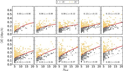
Selection of GAMA groups with apparent richness NFoF ≥ 5 and redshift 0.03 ≤ z < 0.33. In each panel, groups are further split by the average projected distance, 〈R〉, of their satellite galaxies using a spline fit for the median of 〈R〉 (red curves). For brevity, we show only the apparent richnesses up to 20. We plot the spline fit from the first redshift bin in all other bins in grey dashed lines. They are used to guide one's eye to see how spline changes from bin to bin.
The spline fit gives us a limit between the central galaxies with satellites that are on average further apart from (upper half – hereafter 〈R〉+) or closer to (lower half – hereafter 〈R〉−) the BCG. The 〈R〉+ sample has 987 galaxy groups and the 〈R〉− sample 1074 galaxy groups. This provides us, by construction, with two samples that have similar redshift, richness and stellar mass distributions, as can be seen in Fig. 2. The median stellar masses and redshifts are listed in Table 1. As the dark matter haloes are located in different cosmic environments, we also want to check for the presence of apparent trends in our two samples with their environments.
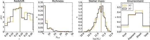
Left-hand panel: Redshift distributions of the GAMA groups used in this paper for both the 〈R〉+ and the 〈R〉− samples, shown as orange and black histograms. Middle left panel: Apparent richness distributions of the GAMA groups used in this paper for both the 〈R〉+ and the 〈R〉− samples. Middle right panel: Stellar mass distributions of the GAMA groups used in this paper for both the 〈R〉+ and the 〈R〉− samples. Right-hand panel: Distribution of the galaxy groups in different cosmic environments. The solid orange and black vertical lines indicate the median of the redshift and stellar mass distributions for the 〈R〉+ and 〈R〉− sample, respectively.
Overview of median stellar masses of central galaxies, median redshifts and number of lenses in each selected sample. Stellar masses are taken from version 16 of the stellar mass catalogue, an updated version of the catalogue created by Taylor et al. (2011).
| Sample | log (〈M⋆/[ M⊙h−1]〉) | 〈z〉 | Number of lenses |
|---|---|---|---|
| Full | 11.32 | 0.188 | 2061 |
| 〈R〉+ | 11.33 | 0.186 | 987 |
| 〈R〉− | 11.30 | 0.190 | 1074 |
| Sample | log (〈M⋆/[ M⊙h−1]〉) | 〈z〉 | Number of lenses |
|---|---|---|---|
| Full | 11.32 | 0.188 | 2061 |
| 〈R〉+ | 11.33 | 0.186 | 987 |
| 〈R〉− | 11.30 | 0.190 | 1074 |
Brouwer et al. (2016) presented a study of galaxies residing in different cosmic environments and they find a clear correlation of the halo bias with the cosmic environment of the haloes the galaxies are residing in. We check for the presence of apparent trends in our two samples, by comparing the distribution of the galaxies residing in voids, sheets, filaments and knots (for the exact definition of the environment classification, see Eardley et al. 2015), and we do not see a large difference (see Fig. 2). It should be noted that the classification of galaxies in Eardley et al. (2015) is only evaluated up to redshift z = 0.263, and because of that this test is only indicative.
3.2 Measurement of the ESD profile
We use imaging data from 180 deg2 of the KiDS (de Jong et al. 2015; Kuijken et al. 2015) that overlaps with the GAMA survey (Driver et al. 2011), to obtain shape measurements of the galaxies. KiDS is a four-band imaging survey conducted with the OmegaCAM CCD mosaic camera mounted at the Cassegrain focus of the VLT Survey Telescope (VST); the camera and telescope combination provides us with a fairly uniform point spread function across the field of view.
From the KiDS data, we use the r-band based shape measurements of galaxies, with an average seeing of 0.66 arcsec. The image reduction, photometric redshift calibration and shape measurement analysis is described in detail in Hildebrandt et al. (2017).
It should be noted that the photometric redshift calibration and shape measurement steps differ significantly from the methods used in Viola et al. (2015) and thus we have to examine the possible systematic errors and biases. In order to do so, we devise a number of tests to see how the data behave in different observational limits, and the results are presented in Appendix A. We test for the presence of additive bias as well as for the presence of cross shear over a wide range of scales. Furthermore, we check how much the GAMA galaxy group members contaminate our source population, and what differences are introduced by the use of a global n(zs) instead of individual p(zs) per galaxy. We conclude that one should use comoving scales between 70 kpc h−1 and 10 Mpc h−1 (this range is motivated by the significant contamination by the GAMA group galaxies on the source population on small scales, and non-vanishing cross-term and additive biases present in the lensing signal calculated around random points on large scales), and use between 5 and 20 radial bins, depending on the choice of error estimation technique and the maximum scale, which is dictated by the number of independent regions one can use to estimate the bootstrap errors and the number of independent entries in the resulting covariance matrix (see further motivation in Section 3.3). Here, we use eight radial bins between 70 kpc h−1 and 10 Mpc h−1. For the sources we adopt the redshift range [0.1, 0.9], motivated by Hildebrandt et al. (2017).
3.3 Covariance matrix estimation
Statistical error estimates on the lensing signal are obtained in two ways. First, we follow the prescription used in Viola et al. (2015) which was shown to be valid in Sifón et al. (2015), van Uitert et al. (2016b) and Brouwer et al. (2016), where we calculate the analytical covariance matrix from the contribution of each source in radial bins. This prescription accounts for shape noise of source galaxies and includes information about the survey geometry (including the masking of the lens and source galaxies). However, this method does not account for sample variance, but Viola et al. (2015) showed that this prescription works sufficiently well up to 2 Mpc h−1. As we calculate the lensing signal up to 10 Mpc h−1, we use the bootstrap method, as the analytical covariance tends to underestimate the errors on scales greater than 2 Mpc h−1 (see Fig. 3, where we compare the different methods for estimating the errors). We first test the bootstrap method by bootstrapping the lensing signal measured around lenses in each of the 1 deg2 KiDS tiles. We randomly select 180 of these tiles with replacement and stack the signals. We repeat this procedure 105 times. The covariance matrix is well constrained by the 180 KiDS tiles used in this analysis, as the number of independent entries in the covariance matrix is equal to 36.
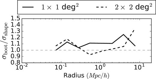
Ratios of the errors obtained using a bootstrap method and the errors obtained from the analytical covariance. Rations for 1 deg2 KiDS tiles and 4 deg2 patches are shown in solid and dashed black lines. The errors are taken as the square root of the diagonal of the respective covariance matrices.
As the physical size of the tile is comparable to the maximum separations, we are considering (one degree at the median redshift of our sample corresponds to ∽8 Mpc h−1), there is a concern that the KiDS tiles might not well describe the errors on scales larger than 2 Mpc h−1, because the tiles are not truly independent from each other. In fact, the sources in neighbouring tiles do contribute to the lensing signal of a group in a certain tile and the tiles are thus not independent on scales above 8 Mpc h−1. We thus repeat the above exercise and calculate the bootstrapped covariance matrix using 4 deg2 KiDS patches (by combining four adjacent KiDS tiles), which leaves us with 45 independent bootstrap regions (which is still enough to constrain the 36 independent entries in our covariance matrix). The square root of diagonal elements compared to the result of the analytical covariance can be seen in Fig. 3 and the full bootstrap correlation matrix in Fig. 4. For a shape noise dominated measurement, one would expect that all three methods yield the same results on scales smaller than 2 Mpc h−1. While this holds for all methods on small scales, it certainly does not hold at scales larger than 2 Mpc h−1 for the analytical and bootstrap covariances, when taking only 1 deg2 tiles. The main issue here is that one lacks large enough independent regions to properly sample the error distribution on large scales, and thus the resulting errors are highly biased. Taking all this considerations into account, we decide to use the bootstrapping over 4 deg2 patches as our preferred method of estimating the errors of our lensing measurements.
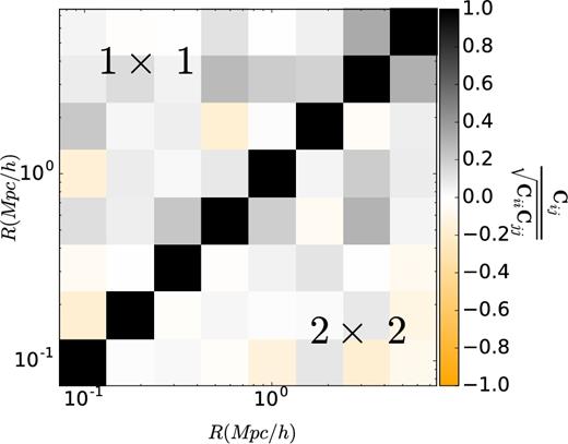
The ESD correlation matrix between different radial bins estimated using a bootstrap technique. Bootstrap covariance accounts both for shape noise and cosmic variance. In the upper triangle we show the correlation matrix when using 1 deg2 tiles, and in the lower triangle the correlation matrix when using 4 deg2 patches (as indicated).
When fitting the halo model to the data, we use the inverse covariance matrix from the bootstrap using 4 deg2 patches. One could use more sophisticated methods to precisely estimate the errors on very large scales. For instance, the analytical covariance method from Hildebrandt et al. (2017) can be adapted for galaxy–galaxy lensing or using galaxy–galaxy lensing specific mock catalogues to estimate the covariance matrix. Future studies using the KiDS data, expanding the analysis over greater separations or simply having more data points should employ methods like that one, but for the purposes of this study, the covariance matrix presented here is sufficient.
4 HALO MODEL
A successful analytic framework to describe the clustering of dark matter and its evolution in the Universe is the halo model (Peacock & Smith 2000; Seljak 2000; Cooray & Sheth 2002; van den Bosch et al. 2013; Mead et al. 2015). The halo model provides an ideal framework to describe the statistical weak lensing signal around a selection of galaxies. One of the assumptions of the halo model is that halo bias is only a function of halo mass, an assumption we want to test in this work. The halo model is built upon the statistical description of the properties of dark matter haloes (namely the average density profile, large scale bias and abundance) as well as on the statistical description of the galaxies residing in them.
4.1 Model specifics
4.2 Fitting procedure
Summary of the lensing results obtained using MCMC halo model fit to the data. All the parameters are defined in Section 4.1. fc is the normalization of the concentration–halo mass relation, poff is the miscentring probability, |${\cal R}_{\rm off}$| is the miscentring distance, M1 is central mass used to parametrize the HOD, σc is the scatter in HOD distribution and b is the bias.
| Sample | log [Mh( M⊙ h−1)] | fc | poff | |${\cal R}_{\rm off}$| | log [M1( M⊙ h−1)] | σc | b |
|---|---|---|---|---|---|---|---|
| Priors | – | [0.0, 6.0] | [0.0, 1.0] | [0.0, 3.5] | [11.0, 17.0] | [0.05, 1.5] | [0.0, 10.0] |
| 〈R〉+ | |$13.32^{+0.13} _{-0.13}$| | |$1.08^{+0.99} _{-0.58}$| | |$0.58^{+0.27}_{-0.36}$| | |$2.10^{+0.99} _{-1.23}$| | |$13.07^{+0.19} _{-0.18}$| | |$0.60^{+0.05} _{-0.05}$| | |$2.77^{+0.78} _{-0.73}$| |
| 〈R〉− | |$13.34^{+0.10} _{-0.11}$| | |$1.61^{+0.99} _{-0.53}$| | |$0.37^{+0.24}_{-0.23}$| | |$2.40^{+0.81} _{-1.50}$| | |$13.10^{+0.17} _{-0.16}$| | |$0.61^{+0.05} _{-0.05}$| | |$3.25^{+0.74} _{-0.74}$| |
| Full | |$13.42^{+0.09} _{-0.08}$| | |$1.03^{+0.63} _{-0.35}$| | |$0.42^{+0.21}_{-0.24}$| | |$2.46^{+0.73} _{-1.24}$| | |$13.22^{+0.14} _{-0.13}$| | |$0.60^{+0.05} _{-0.05}$| | |$3.05^{+0.72} _{-0.75}$| |
Fig. 5 shows the stacked ESD profile for all 2061 galaxy groups (full sample). In comparison to Viola et al. (2015), this sample has around ∽40 per cent more galaxy groups, given by the fact we are using the full equatorial KiDS and GAMA overlap. We calculate the lensing signal for all our samples according to the procedure described in Section 3.2. In the same figure, we also show the halo model fit to the data, as described in this section.
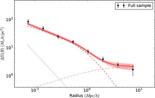
Stacked ESD profiles measured around the central galaxies of GAMA groups from the full sample of galaxies used in this study. The solid red lines represent the best-fitting halo model as obtained using an MCMC fit, with the 68 per cent confidence interval indicated with a shaded region. Dashed, dash–dotted and dotted lines represent the one-halo term, two-halo term and stellar contribution, respectively (see Section 4.1).
5 RESULTS
We fit the halo model as presented in Section 4.1 to the two subsamples (〈R〉+ – sample with more dispersed satellite galaxies and 〈R〉− – sample with more concentrated satellite galaxies). The fits have a reduced |$\chi ^{2}_{{\rm red}}$| (=χ2/degrees of freedom) equal to 1.31 and 1.41 for the 〈R〉+ and 〈R〉− sample, respectively, and the best-fitting models are presented in Fig. 6, plotted with the 16 and 84 percentile confidence intervals. We also plot the stacked ESD profiles for both samples of galaxies, with 1σ error bars, which are obtained by taking the square root of the diagonal elements of the bootstrap covariance matrix.
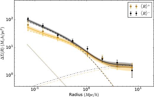
Stacked ESD profiles measured around the central galaxies of GAMA groups, selected according to the average separation of satellite galaxies (see Section 3.1). The solid orange and black lines represent the best-fitting halo model as obtained using an MCMC fit, with the 68 per cent confidence interval indicated with a shaded region. Dashed, dash–dotted and dotted lines represent the one-halo term, two-halo term and stellar contribution, respectively.
The measured parameters are summarized in Table 2, and their full posterior distributions are shown in Fig. B3. The various parameters show similar results between the 〈R〉+ and 〈R〉− subsamples. The normalizations of the concentration–halo mass relations fc are |$f_{{\rm c}}^{+}= 1.08^{+0.99} _{-0.58}$| and |$f_{{\rm c}}^{-} = 1.61^{+0.99} _{-0.53}$| for 〈R〉+ and 〈R〉− respectively, in accordance with the results for the full sample (see Table 2). Furthermore the scatter in halo masses, σc is constrained to ∽0.6 for both samples and it is also consistent with the results for the full sample (see Table 2). We observe lower probabilities for miscentring of the central galaxy than reported in Viola et al. (2015), but with a larger miscentring distance. It should be noted, that the average projected offset αoff (|$\alpha _{{\rm off}} = p_{{\rm off}} \times {\cal R}_{\rm off}$|) is highly degenerate with the concentration normalization fc and the posterior probability distribution is shown in Fig. 7. The resulting degeneracy is similar to the one presented in Viola et al. (2015).
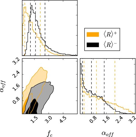
The posterior distributions of the average projected offset αoff and the normalization of the concentration–halo mass relation fc. The contours indicate 1σ and 2σ confidence regions.
Since we consider ESD profiles out to 10 Mpc h−1, the halo masses are well constrained by the innermost part of the same ESD profile (r200 associated with this mass scale is significantly smaller than 10 Mpc h−1). The contribution to the ESD profile beyond 2 Mpc h−1 can be associated purely with the two-halo term (see Fig. 6). The ratio of the obtained halo biases is |$b^{+}/b^{-} = 0.85^{+0.37}_{-0.25}$|. The posterior probability distributions of the obtained halo masses and biases can be seen in Figs 8 and B3.
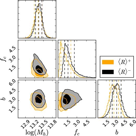
The posterior distributions of the halo model parameters Mh, fc and b. The posterior distributions clearly show a slight difference in the obtained halo masses as well as no difference in the obtained halo biases. The contours indicate 1σ and 2σ confidence regions.
With the lensing measurements providing us the same halo masses for the two samples (within the errors), we report a null detection of halo assembly bias on galaxy groups scales. Our result is in accordance with what one would expect if halo bias is only a function of mass (see Fig. 9). In Fig. 9, we also compare our results with the biases obtained by Miyatake et al. (2016) and to the predictions for a concentration dependent halo bias from Wechsler et al. (2006). To account for the slightly different masses of our two samples one can also compare the difference arising purely from the normalization of the bias Ab (as defined in equation 19). The ratio of obtained normalizations is still compatible with a null detection; |$A_{{\rm b}}^{+} / A_{{\rm b}}^{-} = 0.86^{+0.43}_{-0.28}$| (0.4σ).
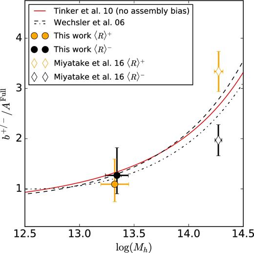
Comparison between the halo bias b and the predictions from the halo bias function from Tinker et al. (2010) and the concentration dependent halo bias from Wechsler et al. (2006), as a function of halo mass Mh. Here circles with error bars show the best-fitting value for b for each sample and diamonds show the results from Miyatake et al. (2016). The halo bias function from Tinker et al. (2010) is shown with a red line and the predictions from Wechsler et al. (2006) for different values of c΄ and a halo collapse mass Mc = 2.1 × 10¹² M⊙ h−1 (as defined therein). The dashed and dash–dotted lines are predictions for c΄ derived for our two samples, 〈R〉+ and 〈R〉−, respectively. Note that the biases are normalized by the Afull.
If the halo assembly bias due to different spatial distributions of satellite galaxies traces the halo bias due to different halo concentrations, then one would expect that the halo assembly bias would follow the predictions presented in Wechsler et al. (2006), and would also not be significant near the halo collapse mass Mc. The halo collapse masses for our two samples are Mc = 2.12 × 10¹² M⊙ h−1 and Mc = 2.02 × 10¹² M⊙ h−1 for the 〈R〉+ and 〈R〉− subsamples, which are ∽8σ below the obtained halo masses. The cancellation effect of the halo assembly bias due to the predicted sign change (clearly seen in Fig. 9) of the concentration dependent halo bias near the Mc cannot be the cause of the null detection of halo assembly bias, as none of our lenses have halo masses that are below the Mc. We however acknowledge that the differences in predicted halo bias following Wechsler et al. (2006) for c΄ (as defined therein) of our two samples at the obtained halo masses are rather small (halo bias ratio of 1.06) and challenging to observe in the first place.
As the results can potentially depend on the choice of the concentration–mass relation, and to see if the choice of our fiducial Duffy et al. (2008) concentration–mass relation does not significantly influence our results, we perform a test where we change the fiducial concentration–mass relation to a parameter that is constant with mass and free to fit. The obtained concentrations for the 〈R〉+ and 〈R〉− subsamples are |$c^{+}= 5.64^{+3.64}_{-2.57}$| and |$c^{-} = 8.36^{+2.38}_{-2.14}$| – again highly degenerate with the average projected offset αoff. The ratio of obtained halo biases in this case is |$b^{+}/b^{-} = 0.86^{+0.41}_{-0.28}$| and the ratio of obtained normalizations is |$A_{{\rm b}}^{+} / A_{{\rm b}}^{-} = 0.89^{+0.45}_{-0.31}$|. We further check if the method presented can detect a bias ratio different than unity using a sample that is known to have one. For this we split our full sample into two samples with different apparent richnesses by making a cut at NFoF = 10 (in order to have two samples with comparable S/N). We fit the halo model as presented in Section 4.1 to obtain the posterior distributions of the halo biases. As expected, the two samples have significantly different halo masses with the high richness sample having a halo mass of |$\log (M_{{\rm h}}[\,\mathrm{M}_{{\odot }} \,h^{-1}]) = 13.72^{+0.13}_{-0.11}$| and the low richness sample having a halo mass of |$\log (M_{{\rm h}}[\,\mathrm{M}_{{\odot }} \,h^{-1}]) = 13.24^{+0.09}_{-0.09}$|. The obtained halo bias ratio is, as expected, different than unity |$b^{{\rm high}}/b^{{\rm low}} = 2.84^{+1.75}_{-1.01}$|, which is also true when one accounts for the fact that the samples have different halo masses. In this case, the ratio of obtained normalizations is |$A_{{\rm b}}^{{\rm high}} / A_{{\rm b}}^{{\rm low}} = 2.14^{+1.42}_{-0.85}$|, which is 1.3σ away from unity. The lensing signal and posterior distributions for this test can be seen in Figs B1 and B2.
6 DISCUSSION AND CONCLUSIONS
We have measured the galaxy–galaxy lensing signal of a selection of GAMA groups split into two samples according to the radial distribution of their satellite galaxies. We use the radial distribution of the satellite galaxies as a proxy for the halo assembly time, and report no evidence for halo assembly bias on galaxy group scales (typical masses of 1013 M⊙ h−1). We use a halo model fit to constrain the halo masses and the large scale halo bias in order to see if the halo biases are consistent with those dictated solely by their halo masses. In this analysis, we used the KiDS data covering 180 deg2 of the sky (Hildebrandt et al. 2017), that fully overlaps with the three GAMA equatorial patches (G9, G12 and G15). As the photometric calibration and shape measurements analysis differ significantly from the previous KiDS data releases, we also perform additional tests for any possible systematic errors and biases that the new procedures might introduce (see Appendix A).
Our findings are in agreement with the results from Zu et al. (2016), who re-analysed the SDSS redMaPPer clusters sample used in Miyatake et al. (2016) and found no evidence for halo assembly bias as previously claimed by Miyatake et al. (2016). They argue that analysis suffered from misidentification of cluster members due to projection effects (Zu et al. 2016), which are minimized in the case when one uses spectroscopic information on cluster or group membership.
It is unlikely that our analysis suffers from the misidentification of the GAMA galaxy groups members and/or contamination from background galaxies to the degree present in the SDSS case (up to 40 per cent, Zu et al. 2016), and thus artificially changing the radial distribution of the satellite galaxies. The projection effects in our case come only from peculiar velocities (and mismatching from the FoF algorithm), whereas the projection effects in Miyatake et al. (2016) are dominated by photo-z uncertainties and errors, which are much larger than peculiar velocities. If that would be the case, this would indeed have a larger effect on groups with a low number of member galaxies (and thus in the same regime we are using for our study). The GAMA groups are, due to available spectroscopic redshifts, highly pure and robust – for groups with NFoF ≥ 5 the purity approaches 90 per cent as assessed using a mock catalogue (Robotham et al. 2011). An issue that remains is the possible fragmentation of the GAMA galaxy groups by the FoF algorithm and a full assessment of this potential issue is beyond the scope of this paper and we defer these topics to a study in the future.
Additionally, the assumption of an NFW profile as our fiducial dark matter density profile can potentially affect the results. Exploration of different profiles is beyond the scope of this paper, but one would not expect that the different profiles would introduce differences in the obtained halo biases. The dark matter density profile does not enter into predictions for the two-halo term which carries all the biasing information. Moreover, any systematic effects due to the differences in profile would enter into both samples in the same way, and when taking the ratio of any quantities, they would to a large extent cancel out.
In order to reach a better precision in our lensing measurements, we could use the full KiDS-450 survey area. This is limited however by the lack of spectroscopy to create a group catalogue. The GAMA survey will be expanded into a newer and upcoming spectroscopic survey named WAVES (Driver et al. 2016),4 which is planned to cover the southern half of the KiDS survey (700 deg2) and provide redshifts for up to 2 million galaxies, which should provide us with enough statistical power not only to access the signatures of assembly bias in those galaxies but to extend the observational evidence also to galaxy scales.
Acknowledgments
We thank the anonymous referee for their very useful comments and suggestions. AD would like to thank to Keira J. Brooks and Christos Georgiou for proof reading the manuscript.
KK acknowledges support by the Alexander von Humboldt Foundation. HH and RH acknowledges support from the European Research Council under FP7 grant number 279396. RN acknowledges support from the German Federal Ministry for Economic Affairs and Energy (BMWi) provided via DLR under project no. 50QE1103. MV acknowledges support from the European Research Council under FP7 grant number 279396 and the Netherlands Organisation for Scientific Research (NWO) through grants 614.001.103. IFC acknowledges the use of computational facilities procured through the European Regional Development Fund, Project ERDF-080 – A supercomputing laboratory for the University of Malta. CH acknowledges support from the European Research Council under grant number 647112. HHi is supported by an Emmy Noether grant (No. Hi 1495/2-1) of the Deutsche Forschungsgemeinschaft. This work is supported by the Deutsche Forschungsgemeinschaft in the framework of the TR33 ‘The Dark Universe’. EvU acknowledges support from an STFC Ernest Rutherford Research Grant, grant reference ST/L00285X/1. AC acknowledges support from the European Research Council under the FP7 grant number 240185.
This research is based on data products from observations made with ESO Telescopes at the La Silla Paranal Observatory under programme IDs 177.A-3016, 177.A-3017 and 177.A-3018, and on data products produced by Target/OmegaCEN, INAF-OACN, INAF-OAPD and the KiDS production team, on behalf of the KiDS consortium.
GAMA is a joint European-Australasian project based around a spectroscopic campaign using the Anglo-Australian Telescope. The GAMA input catalogue is based on data taken from the Sloan Digital Sky Survey and the UKIRT Infrared Deep Sky Survey. Complementary imaging of the GAMA regions is being obtained by a number of independent survey programs including GALEX MIS, VST KiDS, VISTA VIKING, WISE, Herschel-ATLAS, GMRT and ASKAP providing UV to radio coverage. GAMA is funded by the STFC (UK), the ARC (Australia), the AAO, and the participating institutions. The GAMA website is http://www.gama-survey.org.
This work has made use of python (http://www.python.org), including the packages numpy (http://www.numpy.org) and scipy (http://www.scipy.org). The halo model is built upon hmfpython package by Murray, Power & Robotham (2013). Plots have been produced with matplotlib (Hunter 2007) and corner.py (Foreman-Mackey 2016).
Author contributions: All authors contributed to writing and development of this paper. The authorship list reflects the lead authors (AD, MC, KK, MV) followed by two alphabetical groups. The first alphabetical group includes those who are key contributors to both the scientific analysis and the data products. The second group covers those who have made a significant contribution either to the data products or to the scientific analysis.
Throughout the paper we assume that the averaged mass profile of haloes is spherically symmetric, since we measure the lensing signal from a stack of many different haloes with different orientations, which averages out any potential halo triaxiality.
As shown in Robotham et al. (2011), the iterative centre is the most accurate tracer of the centre of group, but using BCG as a tracer is not very different from it.
NFoF is defined by the number of GAMA galaxies associated with the group and it is dependent on the group selection function.
Homepage: http://www.wavesurvey.org
REFERENCES
APPENDIX A: SYSTEMATICS TESTS
We show here additional systematic tests performed as the image reduction procedure, photometric redshift calibration and shape measurement steps differ significantly from the methods used in Viola et al. (2015). We devise a number of tests to see how the obtained data behave in different observational limits, and the results are presented in the following paragraphs.
A1 Multiplicative bias
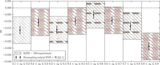
The estimates of the average multiplicative bias m for each redshift slice used in the calculation are obtained using a method presented in Fenech Conti et al. (2016). They are further weighted by the weight w΄ = wsD(zl, zs)/D(zs) for a given lens–source sample. Typically, the value of the μ correction is around −0.014, independent of the scale at which it is computed. Fig. A1 shows the estimates of the average multiplicative bias m for each redshift slice used in the calculation.
A2 Additive bias
Secondly, we test for the presence of the additive shear bias, by checking the tangential shear component measured around random points. This is calculated by performing lensing measurements around 10 million random points in RA and Dec. (for all three GAMA patches), which have the same assigned redshift distribution as the GAMA galaxies. We use version 1 of the GAMA random catalogue, created as described in Farrow et al. (2015). Like the cross component of the measured ellipticities, also the azimuthally averaged tangential shear signal around random points should equal to zero. Figs A2 and A3 show significant systematic errors on scales larger than 1 Mpc h−1 as well as patch-dependent systematic errors. We perform the analysis on three patches separately (G9, G12 and G15). As discussed in Hildebrandt et al. (2017) and Fenech Conti et al. (2016), the correction for the additive bias obtained using image simulations should only be obtained for individual KiDS patches, due to specific systematics associated with each patch. We also check for the behaviour of the cross shear component. Any presence of the cross component signal points towards the presence of systematic errors and thus measurements on scales with significant cross component signal have to be corrected before using them for scientific purposes.
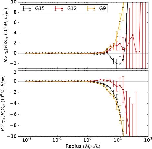
Shear signal around 10 million random points having the same redshift distribution as GAMA galaxies, split between the three GAMA patches. Shown are both tangential (γt, upper panel) and cross (γ× lower panel) components. We use these measurements to correct for the additive bias in our measured ESD signal.
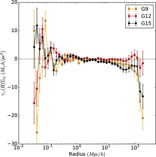
Lensing signal computed from the cross component of measured ellipticities, around all GAMA galaxies in the three equatorial patches (G9, G12 and G15). One can see, that the systematic errors significantly affect the signal below 70 kpc h−1 and above 10 Mpc h−1, with the G12 patch being the least affected, even after subtracting the signal computed around random points.
One could estimate the additive bias using image simulations (using a method shown in Fenech Conti et al. 2016), but that will only account for the PSF effects. We correct for the additive bias using the results obtained from the random signal as the additive bias might arise because of spurious objects (including asteroids, stellar spikes, pixel defects, etc.) in our lensing data, apart from PSF effects. It is thus important to correct for it using the data. Correction of additive bias is performed by subtracting the random signal obtained for each patch from the true ESD measurement in the same patches. Doing so, that also gives better covariance matrix estimates (Singh et al. 2016). The final ESD profile is calculated by combining the random-subtracted signals from all three patches.
A3 Group member contamination of the source galaxies
The next important test we perform is to check how much the GAMA galaxy group members contaminate our source population (the so-called boost factor; Miyatake et al. 2015; van Uitert et al. 2016a). Those galaxies will dilute the lensing signal (as they are not lensed). The resulting lensing signal will be biased (Fig. A4) on small scales with the source overdensity up to 30 per cent at 75 kpc h−1 (Fig. A4). We can impose a more stringent cut than the cut zs > zl used in previous studies on KiDS and GAMA data, by adding an offset δz to the cut on the source population. As seen in Fig. A4, using a conservative cut with δz = 0.1 still leaves a 10 per cent overdensity in the source sample. More conservative cuts lower the observed overdensity, as expected. They also suppress the contamination, but this is not ideal as real source galaxies are removed as well, since it decreases the lensing signal-to-noise. On the small scales (below 75 kpc h−1) the decrease of the source density is connected with the fact that the source galaxies become obscured by the host BCG of the GAMA group. The ESD signals in Fig. A4 are corrected with the boost factor using the factors shown in the top panel of the same figure and have lensing efficiency calculated separately for each redshift cut. We find that for a redshift offset of δz = 0.2 the boost correction is not necessary.
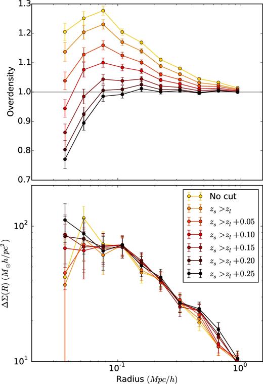
Top panel: The overdensity of KiDS source galaxies around GAMA galaxy groups with richness NFoF ≥ 5. The various lines correspond to different redshift cuts applied to the source sample. Even for a conservative cut of zs > zl + 0.1, we find a residual contamination of group members in the source sample of up to 10 per cent at 75 kpc. Bottom panel: The ESD signal around GAMA galaxy groups with richness NFoF ≥ 5 up to 2 Mpc h−1. The various lines correspond to different redshift cuts applied to the source sample. The redshift cut does not significantly affect the lensing signal, but one removes any possible problems due to group contamination. The lensing signals are computed using different lensing efficiencies and are corrected with the boost factor using the factors shown in the top panel.
A4 Source redshift distribution
The significant difference between this analysis and previous method presented in Viola et al. (2015) is the usage of full redshift probability distribution of the sources, n(zs), compared to Viola et al. (2015) where each source is given its own posterior redshift distribution p(zs) obtained from BPZ. We perform a couple of tests to see what the effect of having only global n(zs) has on the error budget and the resulting lensing signals. The observable lensing signal depends on the angular diameter distances to the lens and source galaxies (equation 9). The redshifts to the lens galaxies are known from the GAMA spectroscopic survey, while for the sources we need to resort to the photometric redshifts derived using multiband images (in ugri photometric bands) of the KiDS survey. The colours obtained using those images are a basis for the photometric redshift estimates, which also provides us the full redshift probability distribution of the sources, n(zs), obtained using the direct calibration method (for more information and comparison with other techniques see Hildebrandt et al. 2017). Comparison between the final lensing signals using the individual p(zs), the stack of p(zs) and the global n(zs) can be seen in the bottom panel of Fig. A5 and the difference between the stacked p(zs) and n(zs) probability distributions in the top panel of the same figure. The resulting lensing signals do not change much, and are all in agreement within the error budget of the lensing signal of all the GAMA galaxies. Following Hildebrandt et al. (2017), we adopt the redshift range [0.1, 0.9], which is the same as the covered range by the four tomographic bins used in Hildebrandt et al. (2017).
![Top panel: Comparison of the n(zs) as given by the direct calibration method (DIR) and the stacked p(zs) obtained from BPZ (Hildebrandt et al. 2017). As already noted in Hildebrandt et al. (2017), the stacked p(zs) does not accurately reproduce the features seen in the DIR method, and its usage is discouraged. Bottom panel: Difference between the lensing signal using three different source redshift distributions. p(zs) represents the method as used in Viola et al. (2015), compared to the stacked p(zs) and the n(zs) obtained using DIR (for all 180 960 GAMA galaxies). Within the error budget, all the methods are in agreement [the orange area is the error on the lensing signal calculated using the n(zs)].](https://oup.silverchair-cdn.com/oup/backfile/Content_public/Journal/mnras/468/3/10.1093_mnras_stx705/1/m_stx705figa5.jpeg?Expires=1750349931&Signature=dsFkfYG5FUDU1cT6FH5AaxfssDmwtX4N04GcA17cCNkxhECLmcyuZxeyazCBRiJvgyzAM9Xj1WNRx1pLOfyOMTSFbbSnxegRUccY0LMVoFMgKdBJ2KVhW4oPMN8~GZH9hIrgkOd~F-1c~RMxfumNCVDPlCgljqeHl~11ix7xbtg6koXnHI778onxvheT0zd49IFFmFYaSCkYR7SVvRYK~G~gF7dEBYNbVIUUYC2rwVmBovuiwc4C8X65xkXU6hYYspi1Aa3BezElerE34kGikLdD6fNgt0mcs9~cA6KPco5BWsCIPQbw5P~e8-7lQBzA4xVvH8NjYKvMbBGlI1jKcw__&Key-Pair-Id=APKAIE5G5CRDK6RD3PGA)
Top panel: Comparison of the n(zs) as given by the direct calibration method (DIR) and the stacked p(zs) obtained from BPZ (Hildebrandt et al. 2017). As already noted in Hildebrandt et al. (2017), the stacked p(zs) does not accurately reproduce the features seen in the DIR method, and its usage is discouraged. Bottom panel: Difference between the lensing signal using three different source redshift distributions. p(zs) represents the method as used in Viola et al. (2015), compared to the stacked p(zs) and the n(zs) obtained using DIR (for all 180 960 GAMA galaxies). Within the error budget, all the methods are in agreement [the orange area is the error on the lensing signal calculated using the n(zs)].
The uncertainty on the n(zs) contributes to the total error budget of the lensing signal. As the errors due to this uncertainty can affect the conclusions of the quantitative results, we look into how much the actual contribution is. We take 1000 bootstrap realizations of the weighted spectroscopic catalogue (Hildebrandt et al. 2017) giving us 1000 different realizations of n(zs), for which we calculate the lensing signal. This gives us enough samples to constrain the uncertainty on the lensing signal due to the uncertainty on the n(zs). We compare the given 1σ errors with the total error on our lensing signal. The results can be seen in Fig. A6, where it is clearly seen that the uncertainty on n(zs) is sub-dominant to the whole error budget.
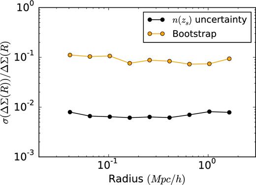
Relative error estimates of the n(zs) uncertainty compared to the uncertainty as obtained using the bootstrap method on the lensing signal (including shape noise and cosmic variance contributions), calculated for the full sample of GAMA galaxies in the three equatorial patches (G9, G12 and G15). It can be seen that the contribution to the total error budget from the uncertainty of the redshift distribution is negligible.
APPENDIX B: FULL POSTERIOR DISTRIBUTIONS
Figs B1 and B2 show lensing signal and posterior distributions of the additional test of splitting the full sample to two samples with high and low richnesses (as discussed in Section 5). In Fig. B3, we show the full posterior probability distribution for all fitted parameters in our MCMC fit as discussed in Sections 4.1 and 5.
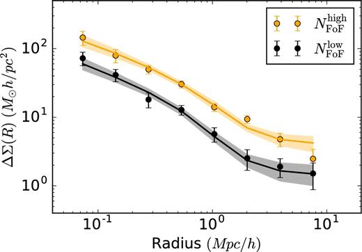
Stacked ESD profiles measured around the central galaxies of GAMA groups, selected according to the apparent richness of the groups. The solid orange and black lines represent the best-fitting halo model as obtained using an MCMC fit, with the 68 per cent confidence interval indicated with a shaded region.
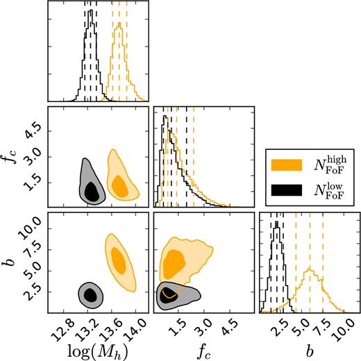
The posterior distributions of the halo model parameters Mh, fc and b for the sample of lenses split according to their apparent richness. The posterior distribution clearly shows a difference in the obtained halo masses as well as a significant difference in the obtained halo biases. The contours indicate 1σ and 2σ confidence regions.
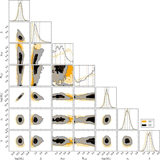
The full posterior distributions of the halo model parameters Mh, fc, poff, |${\cal R}_{\rm off}$|, M1, σc and b. The posterior distribution clearly shows a slight difference in the obtained halo masses as well as no difference in the obtained halo biases, the miscentring parameters and the normalization of concentration–halo mass relation. The contours indicate 1σ and 2σ confidence regions. Priors used in the MCMC fit can be found in Section 4.1.
