


Abstract
We present the first fully simultaneous fits to the near-infrared (NIR) and X-ray spectral slope (and its evolution) during a very bright flare from Sgr A*, the supermassive black hole at the Milky Way's centre. Our study arises from ambitious multiwavelength monitoring campaigns with XMM–Newton, NuSTAR and SINFONI. The average multiwavelength spectrum is well reproduced by a broken power law with ΓNIR = 1.7 ± 0.1 and ΓX = 2.27 ± 0.12. The difference in spectral slopes (ΔΓ = 0.57 ± 0.09) strongly supports synchrotron emission with a cooling break. The flare starts first in the NIR with a flat and bright NIR spectrum, while X-ray radiation is detected only after about 103 s, when a very steep X-ray spectrum (ΔΓ = 1.8 ± 0.4) is observed. These measurements are consistent with synchrotron emission with a cooling break and they suggest that the high-energy cut-off in the electron distribution (γmax) induces an initial cut-off in the optical–UV band that evolves slowly into the X-ray band. The temporal and spectral evolution observed in all bright X-ray flares are also in line with a slow evolution of γmax. We also observe hints for a variation of the cooling break that might be induced by an evolution of the magnetic field (from B ∼ 30 ± 8 G to B ∼ 4.8 ± 1.7 G at the X-ray peak). Such drop of the magnetic field at the flare peak would be expected if the acceleration mechanism is tapping energy from the magnetic field, such as in magnetic reconnection. We conclude that synchrotron emission with a cooling break is a viable process for Sgr A*'s flaring emission.
1 INTRODUCTION
Sgr A*, the supermassive black hole (BH) at the Milky Way's centre, with a bolometric luminosity of L ∼ 1036 erg s−1 is currently characterized by an exceptionally low Eddington ratio (∼10−8; Genzel, Eisenhauer & Gillessen 2010), despite indications that Sgr A* might have been brighter in the past (see Ponti et al. 2013, for a review). Therefore, Sgr A* provides us with the best chance to get a glimpse of the physical processes at work in quiescent BH.
Sgr A* has been intensively studied over the past several decades at various wavelengths. The black points (upper–lower limits) in Fig. 1 show a compilation of measurements of Sgr A*'s quiescent emission from radio to mid-IR (values are taken from Falcke et al. 1998; Markoff et al. 2001; An et al. 2005; Marrone et al. 2006; Schödel et al. 2007, 2011; Dodds-Eden et al. 2009; Bower et al. 2015; Brinkerink et al. 2015; Liu et al. 2016; Stone et al. 2016) as well as the radiatively inefficient accretion flow model proposed by Yuan, Quataert & Narayan (2003). The bulk of Sgr A*'s steady radiation is emitted at sub-mm frequencies, forming the so called ‘sub-mm bump’ (dot–dashed line in Fig. 1). This emission is linearly polarized (2–9 per cent; Marrone et al. 2006, 2007), slowly variable and decreases rapidly with frequency (with stringent upper limits in the mid-IR band; Schödel et al. 2007; Trap et al. 2011). This indicates that the sub-mm radiation is primarily due to optically thick synchrotron radiation originating in the central ∼10RS1 and produced by relativistic (γe ∼ 10, where γe is the electron Lorentz factor) thermal electrons with temperature and densities of Te ∼ few 1010K and ne ∼ 106 cm−3, embedded in a magnetic field with a strength of ∼10–50 G (Loeb & Waxman 2007; Genzel et al. 2010; in Fig. 1 a possible inverse Compton component is also shown). Moreover, Faraday rotation measurements constraint the accretion rate at those scales to be within 2 × 10⁻⁹ and 2 × 10⁻⁷ M⊙ yr−1 (Marrone et al. 2006, 2007; Genzel et al. 2010).
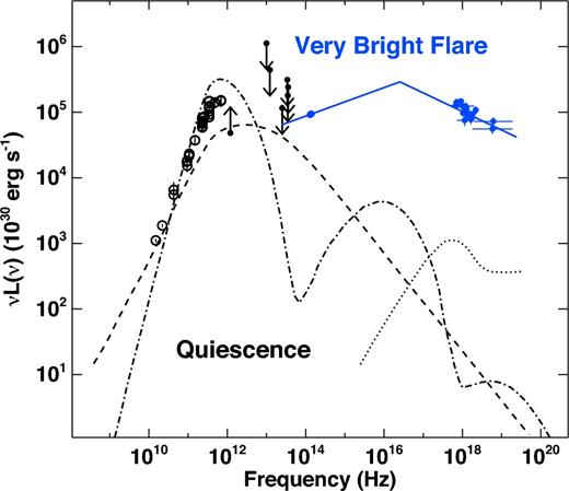
Multiwavelength emission from Sgr A*. The radio to mid-IR data points (open circles as well as upper–lower limits) constrain Sgr A*'s quiescent emission (these constraints are taken from the literature, see text). The black lines show the radiatively inefficient accretion disc model proposed by Yuan et al. (2003). The dash–dotted black line shows the contribution from the thermal electrons with Te ∼ few1010K and ne ∼ 106 cm−3, embedded in a magnetic field with strength of ∼10–50 G producing the sub-mm peak and (possibly) inverse Compton emission at higher energies. The dashed line shows the contribution from a non-thermal tail in the electron population, while the dotted line shows the bremsstrahlung emission from hot plasma at the Bondi radius (Quataert 2002). The blue filled data points show the mean NIR and X-ray spectra of the very bright flare VB3 and the blue solid line shows the best-fitting power law with cooling break (see also Fig. 6).
At low frequency (ν < 1011 Hz), Sgr A*'s SED changes slope (Fν ∝ ν0.2) showing excess emission above the extrapolation of the thermal synchrotron radiation and variability on time-scales of hours to years (Falcke et al. 1998; Zhao et al. 2003, 2004; Herrnstein et al. 2004). This suggests either the presence of a non-thermal tail in the electron population, taking ∼1 per cent of the steady state electron energy (Özel, Psaltis & Narayan 2000; see dashed line in Fig. 1) or a compact radio jet (Falcke et al. 1998; Mościbrodzka et al. 2009, 2014; Mościbrodzka & Falcke 2013). The presence of this non-thermal tail is well constrained at low radio frequencies, while its extrapolation in the mid and near-infrared (NIR) band is rather uncertain (see dashed line in Fig. 1).
Sgr A* also appears as a faint (L2−10 keV ∼ 2 × 1033 erg s−1) X-ray source (Baganoff et al. 2003; Xu et al. 2006) observed to be extended with a size of about ∼1 arcsec. The observed size is comparable to the Bondi radius and the quiescent X-ray emission is thought to be the consequence of material that is captured at a rate of 10−6 M⊙ yr−1 from the wind of nearby stars (Melia 1992; Quataert 2002; Cuadra et al. 2005, 2006; Cuadra, Nayakshin & Martins 2008). Indeed, this emission is thought to be produced via bremsstrahlung emission from a hot plasma with T ∼ 7 × 10⁷ K, density ne ∼ 100 cm−3 emitted from a region ∼105RS (Quataert 2002; see dotted line in Fig. 1).
For more than a decade, it has been known that Sgr A* also shows flaring activity both in X-rays and IR (Baganoff et al. 2001; Genzel et al. 2003; Goldwurm et al. 2003; Porquet et al. 2003, 2008; Eckart et al. 2004, 2006; Ghez et al. 2004; Bélanger et al. 2005; Marrone et al. 2008; Haubois et al. 2012; Nowak et al. 2012; Degenaar et al. 2013; Neilsen et al. 2013, 2015; Barrière et al. 2014; Mossoux et al. 2015; Ponti et al. 2015c; Yuan & Wang 2016). X-ray flares appear as clear enhancements above the constant quiescent emission, with peak luminosities occasionally exceeding the quiescent luminosity by up to two orders of magnitude (see the blue points in Fig. 1 for an example of a very bright flare; Baganoff et al. 2001; Porquet et al. 2003, 2008; Nowak et al. 2012). X-ray flare durations, fluences and peak luminosities are correlated (Neilsen et al. 2013). Moreover, weak X-ray flares are more common than strong ones (Neilsen et al. 2013; Ponti et al. 2015c). The appearance of the X-ray light curves suggests that flares are individual and distinct events, randomly punctuating an otherwise quiescent source (Neilsen et al. 2013; Ponti et al. 2015c).
Typically X-ray flares coincide with clear peaks in the NIR light curves (e.g. Genzel et al. 2003; Clénet et al. 2004; Ghez et al. 2004; Eckart et al. 2006, 2008; Meyer et al. 2006, 2007, 2008; Yusef-Zadeh et al. 2006, 2009; Hornstein et al. 2007; Do et al. 2009). However, the appearance of the NIR light curves is significantly different from the X-ray ones. Indeed, the NIR and sub-mm emission of Sgr A* are continuously varying and they can be described by a red noise process at high frequencies, breaking at time-scales longer than a fraction of a day2 (Do et al. 2009; Meyer et al. 2009; Dodds-Eden et al. 2011; Witzel et al. 2012; Dexter et al. 2014; Hora et al. 2014). Therefore, the NIR light curves do not support the notion of flares as individual events; they would alternatively corroborate the concept that flares are simply peaks of emission on a continuous red noise process. Despite the fact that the notion of NIR-flares is still unsettled, we will refer to the X-ray flares, and by extension, to the NIR peaks in emission, as flares throughout this paper.
The origin and radiative mechanism of the flares of Sgr A* are still not completely understood. Several multiwavelength campaigns have been performed, but the radiative mechanisms at work during the flares is still highly debated (Eckart et al. 2004, 2006, 2008, 2009, 2012; Yusef-Zadeh et al. 2006, 2008, 2009; Hornstein et al. 2007; Marrone et al. 2008; Dodds-Eden et al. 2009; Trap et al. 2011; Barrière et al. 2014). Indeed, even though 15 yr have passed since the launch of XMM–Newton and Chandra, simultaneous X-ray and NIR spectra of a bright flare (as these allow a precise determination of the spectral index in the two bands) have not yet been published.3
Polarization in the sub-mm and NIR bands suggests that the NIR radiation is produced by synchrotron emission. The origin of the X-ray emission is still debated. Indeed, the X-ray radiation could be produced by synchrotron itself or inverse Compton processes such as synchrotron self-Compton or external Compton (see Genzel et al. 2010, for a review). Different models explain the data with a large range of physical parameters; however, models with synchrotron emission extending with a break from NIR to the X-ray seem to be best able to account for the X-ray data with reasonable physical parameters (Dodds-Eden et al. 2009; Trap et al. 2010; Barrière et al. 2014; Dibi et al. 2014, 2016).
We report here the first simultaneous observation of the X-ray (XMM–Newton), hard X-ray (NuSTAR) and NIR (SINFONI) spectra of a very bright flare of Sgr A*, which occurred between 2014 August 30 and 31 (Ponti et al. 2015b,c), and an analysis of flare models which could explain the emission. The remainder of this paper is organized as follows: Section 2 details the reduction of the X-ray and NIR data. In Section 3, we present a characterization of the obscuration and mean spectral properties of the very bright flares observed by XMM–Newton. In Section 4, we investigate the mean properties of the VB3 flare, in particular we constrain the radiative mechanism through the study of the mean multiwavelength spectrum. In Section 5, we follow the evolution of the flare emission to determine time-dependent parameters of the emission models. Section 6 scrutinizes a ‘quiescent’ interval after the very bright flare. In Section 7, we focus the analysis on the X-ray band only and we study the evolution of the X-ray spectral shape throughout all bright and very bright X-ray flares. We discuss the results of the model fits in Section 8 and conclude in Section 9.
2 DATA REDUCTION
We consider two sets of data in this paper. The first set comprises simultaneous X-ray (XMM–Newton and NuSTAR) and NIR data of one very bright flare, called VB3 (see Ponti et al. 2015c for the definition of the naming scheme). The analyses of the XMM–Newton, NuSTAR and SINFONI data on flare VB3 are discussed in Sections 2.2, 2.3 and 2.4. The second set of data consists of all of Sgr A*'s bright or very bright X-ray flares as detected with XMM–Newton. The reduction of this set of data is discussed in Section 2.2 along with the description of the flare VB3.
2.1 Basic assumptions
Throughout the paper we assume a distance to Sgr A* of 8.2 kpc and a mass of M = 4.4 × 10⁶ M⊙ (Genzel et al. 2010). The errors and upper limits quoted on spectral fit results correspond to 90 per cent confidence level for the derived parameters (unless otherwise specified), while uncertainties associated with measurements reported in plots are displayed at the 1σ confidence level. The neutral absorption affecting the X-ray spectra is fitted with the model TBnew4 (see Wilms, Allen & McCray 2000) with the cross-sections of Verner et al. (1996) and abundances of Wilms et al. (2000). The dust scattering halo is fitted with the model fgcdust in xspec (Jin et al. 2017; see section 3) and it is assumed to be the same as the ‘foreground’ component along the line of sight towards AX J1745.6−2901 (Jin et al. 2017). More details on the implications of this assumptions are included in Section 3 and Appendix B. In Section 3, we justify the assumption of a column density of neutral absorbing material of NH = 1.60 × 1023 cm−2 and we apply it consistently thereafter. Throughout our discussion we assume that the effects of beaming are negligible, as well as a single zone emitting model for the source.
Unless otherwise stated, we follow Dodds-Eden et al. (2009) and we assume a constant escape time of the synchrotron emitting electrons equal to tesc = 300 s. Under this assumption, the frequency of the synchrotron cooling break can be used to derive the amplitude of the source magnetic field.
2.2 XMM–Newton
In this work, we considered all of the XMM–Newton observations during which either a bright or very bright flare has been detected through the Bayesian block analysis performed by Ponti et al. (2015c). Full details about the observation identification (obsID) are reported in Table 1.
List of XMM–Newton observations and flares considered in this work. The flares are divided into two categories, bright (B) and very bright (VB), classified according to their total fluence (see Ponti et al. 2015c). The different columns show the XMM–Newton obsID, flare start and end times in terrestrial time (TT‡; see Appendix A) units and flare name, respectively. The flare start and end times are barycentric corrected (for comparison with multiwavelength data) and correspond to the flare start time (minus 200 s) and flare stop time (plus 200 s) obtained through a Bayesian block decomposition (Ponti et al 2015c; please note that the time stamps in Ponti et al 2015c are not barycentric corrected). Neither a moderate nor weak flare is detected during these XMM–Newton observations. To investigate the presence of any spectral variability within each very bright flare, we extracted three equal duration spectra catching the flare rise, peak and decay, with the exception of VB3. In the latter case, we optimized the duration of these time intervals according to the presence of simultaneous NIR observations (see Fig. 5).
| XMM–Newton | Date | tstart | tstop | NAME |
|---|---|---|---|---|
| obsID | TTTBD | TTTBD | ||
| Archival data | ||||
| 0111350301 | 2002 October 3 | 150026757 | 150029675 | VB1 |
| 150026757 | 150027730 | VB1-Rise | ||
| 150027730 | 150028702 | VB1-Peak | ||
| 150028702 | 150029675 | VB1-Dec | ||
| 0402430401 | 2007 April 4 | 292050970 | 292054635 | VB2 |
| 292050970 | 292052192 | VB2-Rise | ||
| 292052192 | 292053413 | VB2-Peak | ||
| 292053413 | 292054635 | VB2-Dec | ||
| 292084140 | 292087981 | B1 | ||
| 0604300701 | 2011 March 30 | 417894177 | 417896560 | B2 |
| This campaign | ||||
| 0743630201 | 2014 August 30 | 525829293 | 525832367 | VB3 |
| 525827793 | 525829193 | VB3-Pre | ||
| 525829193 | 525830593 | VB3-Rise | ||
| 525830593 | 525831843 | VB3-Peak | ||
| 525831843 | 525832743 | VB3-Dec | ||
| 525832743 | 525834893 | VB3-Post | ||
| 2014 August 31 | 525846661 | 525848532 | B3 | |
| 0743630301 | 2014 September 01 | 525919377 | 525924133 | B4 |
| 0743630501 | 2014 September 29 | 528357937 | 528365793 | B5 |
Starting from the XMM–Newton observation data files, we reprocessed all of the data sets with the latest version (15.0.0) of the XMM–Newton Science Analysis System (sas), applying the most recent (as of 2016 April 27, valid for the observing day) calibrations. Whenever present, we eliminated strong soft proton background flares, typically occurring at the start or end of an observation, by cutting the exposure time as done in Ponti et al. (2015c; see Table 7). To compare data taken from different satellites and from the ground, we performed barycentric correction by applying the BARYCEN task of sas. The errors quoted on the analysis of the light curves correspond to the 1σ confidence level (unless otherwise specified). xspec v12.8.2 and matlab are used for the spectral analysis and the determination of the uncertainties on the model parameters.
We extracted the source photons from a circular region with 10 arcsec radius, corresponding to ∼5.1 × 10⁴ au, or ∼6.5 × 10⁵RS (Goldwurm et al. 2003; Bélanger et al. 2005; Porquet et al. 2008; Trap et al. 2011; Mossoux et al. 2015). For each flare, we extracted source photons during the time window defined by the Bayesian block routine (applied on the EPIC-pn light curve, such as in Ponti et al. 2015c), adding 200 s before and after the flare (see Table 1). Background photons have been extracted from the same source regions by selecting only quiescent periods. The latter are defined as moments during which no flare of Sgr A* is detected by the Bayesian block procedure (Ponti et al. 2015c) and additionally leaving a 2 ks gap before the start and after the end of each flare.
Given that all of the observations were taken in full frame mode, pile-up is expected to be an issue only when the count rate exceeds ∼2 cts s−1.5 This threshold is above the peak count rate registered even during the brightest flares of Sgr A*. This provides XMM–Newton with the key advantage of being able to collect pile-up free, and therefore unbiased, spectral information even for the brightest flares.
For each spectrum, the response matrix and effective area have been computed with the xmm-sas tasks RMFGEN and ARFGEN. See Appendix A for further details on the XMM–Newton data reduction.
2.3 NuSTAR
To study the flare characteristics in the broad X-ray band, we analysed the two NuSTAR observations (obsID: 30002002002, 30002002004) taken in fall 2014 in coordination with XMM–Newton (Table 2). We processed the data using the NuSTAR Data Analysis Softwarenustardas v. 1.3.1. and heasoft v. 6.13, filtered for periods of high instrumental background due to SAA passages and known bad detector pixels. Photon arrival times were corrected for onboard clock drift and precessed to the Solar system barycentre using the JPL-DE200 ephemeris. For each observation, we registered the images with the brightest point sources available in individual observations, improving the astrometry to ∼4 arcsec. We made use of the data obtained by both focal plane modules FPMA and FPMB.
Four XMM–Newton flares were captured in the coordinated NuSTAR observations: VB3, B3, B4 and B5. We extract the NuSTAR flare spectra using the same flaring intervals as determined from the XMM–Newton data (see Table 1). The flare times are barycentric corrected for comparison between different instruments. Due to interruption caused by earth occultation, NuSTAR good time intervals (GTIs) detected only a portion of the flares. For flare VB3, NuSTAR captured the first ∼1215 s of the full flare, corresponding to pre-, rising- and part of the peak-flare, while the dec- and post-flare intervals were missed. Similarly, part of the rising-flare stage of flare B3 and the middle half of flare B4 were captured in the NuSTAR GTIs. Flare B5 was not significantly detected with NuSTAR, resulting in ∼2σ detection in the NuSTAR energy band.
To derive the flare spectra, we used a source extraction region with 30 arcsec radius centred on the position of Sgr A*. While the source spectra were extracted from the flaring intervals, the background spectra were extracted from the same region in the off-flare intervals within the same observation. The spectra obtained by FPMA and FPMB are combined and then grouped with a minimum of 3σ signal-to-noise significance per data bin, except the last bin at the high-energy end for which we require a minimum of 2σ significance.
2.4 SINFONI
2.4.1 Observations and data reduction
We observed Sgr A* with SINFONI (Eisenhauer et al. 2003; Bonnet et al. 2004) at VLT between 2014 August 30 23:19:38 UTC and 2014 August 31 01:31:14 UTC. SINFONI is an adaptive optics (AO) assisted integral-field spectrometer mounted at the Cassegrain focus of Unit Telescope 4 (Yepun) of the ESO very large telescope. The field of view used for this observation was 0.8 arcsec × 0.8 arcsec, which is divided into 64 × 32 spatial pixels by the reconstruction of the pseudo-slit into a 3D image cube. We observed in H + K bands with a spectral resolution of ∼1800.
We accumulated seven spectra (see observation log in Table 3) of 600 s each using an object-sky-object observing pattern. There are gaps between observations for the 600 s sky exposures, as well as a longer gap due to a brief telescope failure during what would have been an additional object frame at the peak of the X-ray flare. In total, we accumulated four sky frames on the sky field (712 arcsec west, 406 arcsec north of Sgr A*). During our observations, the seeing was ∼0.7 arcsec and the optical coherence time was ∼2.5 ms. The AO loop was closed on the closest optical guide star (mR = 14.65; 10.8 arcsec east, 18.8 arcsec north of Sgr A*), yielding a spatial resolution of ∼90 mas full width at half-maximum (FWHM) at 2.2 μm, which is ∼1.5 times the diffraction limit of UT4 in K band.
The reduction of the SINFONI data followed the standard steps. The object frames were sky subtracted using the nearest-in-time sky frame to correct for instrumental and atmospheric backgrounds. We applied bad pixel correction, flat-fielding and distortion correction to remove the intrinsic distortion in the spectrograph. We performed an initial wavelength calibration with calibration source arc lamps, and then fine-tuned the wavelength calibration using the atmospheric OH lines of the raw frames. Finally, we assembled the data into cubes with a spatial grid of 12.5 mas per pixel.
2.4.2 Sgr A* spectrum extraction
The source spectrum extraction uses a procedure to extract a noisy spectrum from Sgr A*. This can then be binned and the scatter within a bin used as an estimate of the error on the flux in that bin. In each of the seven data cubes, we use a rectangular region of the spatial dimensions of size (0.31 arcsec × 0.36 arcsec) centred roughly between Sgr A* and the bright star S2 (0.05 arcsec south of S2). Within this region are four known S-stars, S2, S17, S19 and S31. Fig. 2 shows a combined data cube assembled from the seven observations, as well as a simulated image of the Galactic Centre S-stars. The four known stars used in the fitting procedure are labelled in both images. We extract ∼100 noisy images from the data cube by collapsing the cube along the spectral direction (median in the spectral direction) in bins with 3.5 nm width (seven spectral channels per bin) in the spectral range 2.03–2.39 μm. This initial binning is necessary, as the signal to noise of a single spectral channel is not high enough on its own to perform the next step.
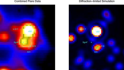
The GC as seen with SINFONI (each image is 0.51 arcsec × 0.61 arcsec). The image on the left is the collapsed image from the spectral range 2.25–2.35 μm for the seven data cubes combined. The image on the right is a diffraction-limited simulated image of the locations of the S-stars in the GC. In both images, the location of Sgr A* is indicated with a cross, and the four stars included in our Gaussian fits for spectrum extraction are labelled with circles. The flare is clearly visible above the background in the left image.
In each noisy image, we determine the flux of Sgr A* from a fit with six Gaussians to the image. Five Gaussians with a common (variable) width describe the five sources in each image. The sixth Gaussian has a width of 3.5 times wider than the sources, and describes the AO seeing halo of the brightest star, S2, which has a K magnitude of ∼14. The seeing haloes of the dimmer stars (K magnitude <15) are neglected in the fit. The positions of the four stars relative to one another and to Sgr A* are fixed based on the known positions of the stars. The flux ratios of the four stars are fixed based on previous photometric measurements of the stars. Note that fixing the flux ratios assumes that the spectral indices of the various S-stars are not significantly different, an excellent assumption given the strong extinction towards the Galactic Centre (GC).
The final fit has five free parameters: The overall amplitude of the S-stars, the background, the Gaussian width of the sources, the flux ratio of the seeing halo/S2 and the flux ratio of Sgr A*/S2. This fitting procedure allows a measurement of the variability of Sgr A* in the presence of variations (in time and wavelength) in the background, Strehl ratio and seeing. The result of this procedure is a flux ratio of Sgr A*/S2 in each of the ∼100 spectral bins.
We obtain a noisy, colour-corrected spectrum of Sgr A* by multiplying a calculated spectrum of S2 by the flux ratio Sgr A*/S2 obtained from the fit in each extracted image. The calculated S2 spectrum used is νSν for a blackbody with a temperature of 25 000 K, and a stellar radius of 9.3R⊙, the best-fitting temperature and radius for S2 found in Martins et al. (2008). The source is placed at 8.2 kpc (Genzel et al. 2010) from the Earth. This spectrum is normalized to a value of 20 mJy at 2.2 μm wavelength to match previous photometric measurements of S2. This procedure corrects for the effects of interstellar extinction. Note that by normalizing the spectrum of S2 to a value of 20 mJy at 2.2 μm, we do not take into account the error on the previous measurements of the flux of S2. Since errors on this value result only in an overall error on the amplitude and not in the spectral shape, this additional uncertainty in the normalization of the spectra is taken into account in the later model fits by allowing the overall amplitude of the NIR spectrum to vary and determining the effect of this variation on the fit parameters.
To obtain the final NIR data points used for the model fitting in this paper, the noisy spectrum is binned into 10 spectral bins (median of the values in each bin) of width 35 nm. The error on each point is the standard deviation of the sample, or |$\sigma /\sqrt{N}$|. We have tested varying the number of initial spectral samples used to create the extracted images used for fitting Sgr A*/S2, and find that it has almost no effect on the final data values and only a small effect on the derived error bars. We have also tried fixing parameters in the fits to determine their effects on the final spectra. We tried fixing the FWHM of the Gaussians and the background level (which both naturally vary with wavelength) to their median values, and found that this affects the spectral index of the final data points by at most a few per cent.
3 X-RAY OBSCURATION AND MEAN X-RAY PROPERTIES OF BRIGHT FLARES
We started the study of Sgr A*'s emission by investigating the properties of the absorption-scattering layers that distort its spectrum.
3.1 Dust scattering
Scattering on dust grains along the line of sight can have a significant impact on the observed X-ray spectra (Predehl & Schmitt 1995; Smith, Valencic & Corrales 2016). The main effect of dust scattering is to create a halo around the source, by removing flux from the line of sight. Both the flux in the halo and its size decrease with energy (with a dependence of ∝E−2 and ∝E−1, respectively) as a consequence of the probability of scattering that drops steeply with energy. If the events used to extract the source photons are selected from a small region containing only a small part of the halo, such as typically the case for X-ray observations of Sgr A*, then the spectral shape will be distorted by the effects of dust scattering. Whenever the distortions are not accurately accounted for, this will cause significant biases in the measured absorption column densities, source brightness and spectral slopes (see Appendix B).
Frequently used models, aimed at mitigating the effects of dust scattering, are dust (Predehl & Schmitt 1995), scatter (Porquet et al. 2003, 2008; Dodds-Eden et al. 2009) and dustscat (Baganoff et al. 2003; Nowak et al. 2012). In all these models, the dust optical depth and therefore the magnitude of the correction, is assumed to be proportional to the X-ray absorbing column density, with a factor derived from Predehl & Schmitt (1995). The underlying assumption is that the dust properties (e.g. dust to gas ratio, size distribution, composition, etc.) towards Sgr A* are equal to the average estimate derived from the study of all the Galactic sources considered in the work of Predehl & Schmitt (1995). After considering the limitations of this approach, we decided to use a completely different method.
Thanks to the analysis of all the XMM–Newton and Chandra observations of the GC, Jin et al. (2017) just completed the accurate characterization of the dust scattering halo towards AX J1745.6−2901, a bright X-ray binary located only ∼1.45 arcmin from Sgr A*. The authors deduced that 74 ± 7 per cent of the dust towards AX J1745.6−2901 resides in front of the GC (e.g. in the spiral arms of the Galaxy). Moreover, the detailed modelling of the dust scattering halo allowed Jin et al. (2017) to provide an improved model of the spectral distortions generated by the dust scattering (fgcdust), without the requirement to assume fudge scaling factors. We therefore decided to fit Sgr A*'s spectrum with the fgcdust model, implicitly assuming that the dust has similar properties along the line of sight towards Sgr A* and the foreground component in the direction of AX J1745.6−2901. This is corroborated by the study of the radial and azimuthal dependence of the halo. In fact, the smoothness of the profile indicates that the foreground absorption has no major column density variations within ∼100–150 arcsec from AX J1745.6−2901 (Jin et al. 2017). Further details on the spectral distortions (and their correction) introduced by dust scattering are discussed in Appendix B.
3.2 Foreground absorption towards the bright sources within the central arcmin
We review here the measurements of the X-ray column density of neutral/low-ionized material along the line of sights towards compact sources located close to Sgr A*. Due to the variety of assumptions performed in the different works (e.g. absorption models, abundances, cross-sections, dust scattering modelling, etc.), we decided to refit the spectra to make all measurements comparable with the abundances, cross-sections and absorption models assumed in this work (see Section 2.1; fig. 5 and table 2 of Ponti et al. 2015a, 2016a).
The different columns show the NuSTAR obsID, observation start time, total exposure, coordinated XMM–Newton obsID and the flares detected in the observation.
| Coordinated NuSTAR and XMM–Newton observations and flares detected | ||||
|---|---|---|---|---|
| NuSTAR obsID | tstart | Exposure (ks) | Joint XMM–Newton obsID | NAME |
| 30002002002 | 2014 August 30 19:45:07 | 59.79 ks | 0743630201 | VB3, B3 |
| 0743630301 | B4 | |||
| 30002002004 | 2014 September 27 17:31:07 | 67.24 ks | 0743630501 | B5 |
AX J1745.6−2901 located at ∼1.45 arcmin from Sgr A*. AX J1745.6−2901 is a dipping and eclipsing neutron star low mass X-ray binary (Ponti et al. 2016). Such as typically observed in high inclination low mass X-ray binaries, AX J1745.6−2901 shows both variable ionized and neutral local absorption (Ponti et al. 2015a). The total neutral absorption column density towards AX J1745.6−2901 has been measured by Ponti et al. (2015a). We refitted those spectra of AX J1745.6−2901 with the improved correction for the dust scattering distortions. By considering that only 74 ± 7 per cent of the dust towards AX J1745.6−2901 resides in front of the GC (Jin et al. 2017), we measured a total column density in the foreground component6 of NH = (1.7 ± 0.2) × 1023 cm−2. We note that the halo associated to the foreground component is still detected at radii larger than r > 100 arcsec (Jin et al. 2017), therefore from a radius more than ten times larger than the one chosen to extract Sgr A*'s photons, indicating that a careful treatment of the distortions introduced by dust scattering is essential.
SWIFT J174540.7−290015 located at ∼16 arcsec from Sgr A*. A deep XMM–Newton observation performed during the recent outburst of Swift J174540.7−290015 (Reynolds et al. 2016), allowed Ponti et al. (2016) to measure the column density along this line of sight and to find NH = (1.70 ± 0.03) × 1023 cm−2, by fitting the spectrum with the sum of a blackbody plus a Comptonization component.7 By applying the improved modelling of the dust scattering halo to the same data, we measured a column density of NH = (1.60 ± 0.03) × 1023 cm−2.
SGR J1745−2900 located at ∼2.4 arcsec from Sgr A*. SGR J1745−2900 is a magnetar located at a small projected distance from Sgr A* (Mori et al. 2013; Kennea et al. 2013), and it is most likely in orbit around the supermassive BH (Rea et al. 2013). Coti-Zelati et al. (2015) fitted the full XMM–Newton and Chandra data set available on SGR J1745−2900, without considering the effects of the dust scattering halo, and found NH = (1.90 ± 0.02) × 1023 cm−2 for Chandra and |$N_{\rm H}=(1.86^{+0.05}_{-0.03})\times 10^{23}$| cm−2 for XMM–Newton. We refitted the XMM–Newton data set at the peak of emission (obsID: 0724210201), using as background the same location when the magnetar was in quiescence and considering the improved dust model, and we obtained |$N_{\rm H}=(1.69^{+0.17}_{-0.10})\times 10^{23}$| cm−2.
Radio observations of the pulsed emission from SGR J1745−2900 allowed Bower et al. (2014) to provide a full characterization of the scattering properties of the absorption. The authors found the obscuring–scattering layer to be located in the spiral arms of the Milky Way, most likely at a distance Δ = 5.8 ± 0.3 kpc from the GC (however a uniform scattering medium was also possible). Moreover, the source sizes at different frequencies are indistinguishable from those of Sgr A*, demonstrating that SGR J1745−2900 is located behind the same scattering medium of Sgr A*.
We note that the column densities of absorbing material along the line of sights towards SWIFT J174540.7−290015, SGR J1745−2900 and the foreground component towards AX J1745.6−2901 are consistent (to an uncertainty of ∼2–10 per cent) within each other. Of course, the neutral absorption towards these accreting sources might even, in theory, be local and variable (e.g. Díaz-Trigo et al. 2006; Ponti et al. 2012a, 2016b); however, the similar values observed in nearby sources indicate a dominant interstellar medium (ISM) origin. We note that the location of the scattering medium towards Sgr A* and the foreground component of AX J1745.6−2901 are also cospatial. This suggests that all these sources are absorbed by a common, rather uniform, absorbing layer located in the spiral arms of the Milky Way (Bower et al. 2014; Jin et al. 2017). This result is also in line with the small spread, of the order of ∼10 per cent, in the extinction observed in NIR towards the central ∼20 arcsec of the Galaxy (Schödel et al. 2010; Fritz et al. 2011). Indeed, for a constant dust to gas ratio, this would induce a spread in the X-ray determined NH of a similarly small amplitude. In addition to this layer, AX J1745.6−2901 also shows another absorbing component, located closer to the source, possibly associated either with the clouds of the central molecular clouds or a local absorption (Jin et al. 2017).
Studies of the scattering sizes from large-scale (∼2°) low frequency radio maps also agree with the idea that the intervening scattering in the GC direction is composed of two main absorption components, one uniform on a large scale and one patchy at an angular scale of ∼10 arcmin and with a distribution following the clouds of the central molecular zone (Roy 2013).
3.3 The mean spectra of the XMM–Newton very bright flares
We extracted an EPIC-pn and EPIC-MOS spectra for each of the bright and very bright flares detected by XMM–Newton. We used a Bayesian block decomposition of the EPIC-pn light curve to define the start and end flare times (see Table 1). We fitted each spectrum with a power-law model modified by neutral absorption (see Section 2.1) and by the contribution from the dust scattering halo (fgcdust * TBnew * power-law in xspec).
Each spectrum is well fitted by this simple model (see Table 4). In particular, the column density of absorption material and the photon index are consistent with being the same between the different flares and consistent with the values observed in nearby sources (see Section 3.2). This agrees with the idea that most of the neutral absorption column density observed towards Sgr A* is due to the ISM. If so, the absorption should not vary significantly over time (see Table 4). Therefore, we repeat the fit of the spectra assuming that the three very bright flares are absorbed by the same column density of neutral material. The three spectra are well described by this simple model (see Table 4), significantly reducing the uncertainties. The best-fitting spectral index is ΓVB123 = 2.20 ± 0.15, while the column density is: NH = (1.59 ± 0.15) × 1023 cm−2.
This value is fully consistent with the one observed towards the foreground component towards bright nearby X-ray sources, reinforcing the suggestion that the column density is mainly due to the ISM absorption. For this reason hereafter we will fix it to the most precisely constrained value NH = 1.60 ± 0.03 × 1023 cm−2 (Ponti et al. 2016a). The resulting best-fitting photon index with this value of NH is |$\Gamma _{\text{VB}123_{\text{Fix}N_{\text{H}}}}=2.21\pm 0.09$|.
4 MEAN PROPERTIES OF VB3
We investigate here the mean properties of a very bright flare (VB3, see Ponti et al. 2015c) during which, for the first time, simultaneous time-resolved spectroscopy in NIR and X-rays has been measured.
4.1 X-ray (XMM–Newton and NuSTAR) mean spectra of VB3
We first simultaneously fitted the XMM–Newton (pn and both MOS) and NuSTAR mean spectra of VB3 (see Fig. 3, Table 1) with an absorbed power-law model. The NuSTAR data cover only part of the flare, missing the decaying flank of the flare, therefore probing different stages of a variable phenomenon. We accounted for this by allowing the fit to have different power-law normalization between the NuSTAR and XMM–Newton spectra.8 The best-fitting photon index is: ΓXMM+Nu = (2.27 ± 0.12) and absorbed 2–10 keV flux F2–10 = 7.5 ± 1.5 × 10⁻¹² erg cm−2 s−1. The spectra were very well fitted by this simple model with χ2 = 141.4 for 133 dof.
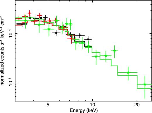
Mean X-ray spectrum of VB3. The black squares, red circles and green stars show the EPIC-pn, combined EPIC-MOS and combined NuSTAR spectra, respectively. The combined XMM–Newton and NuSTAR spectra greatly improve the determination of the X-ray slope. The data are fitted with an absorbed power law model, which takes into account the distortions induced by the dust scattering (see text for more details).
We investigated for the presence of a possible high-energy cut-off (or high-energy spectral break) by fitting the spectra with an absorbed broken power-law (BPL) model. We fixed the photon index of the lower energy power-law slope to |$\Gamma _{\text{VB}123_{\text{Fix}N_{\text{H}}}}=2.20$| (the best-fitting value of the simultaneous fit of VB1+VB2+VB3, see Table 4). No significant improvement was observed (χ2 = 141.2 for 132 dof).
4.2 Multiwavelength mean spectra of VB3
We then extended our investigation by adding the NIR spectra. Multiple SINFONI spectra (e.g. IR2, IR3 and IR4) have been accumulated during the duration of the X-ray emission of the VB3 flare9 (see Fig. 5). Therefore, we created the mean spectrum from these NIR spectra and fitted these simultaneously with the mean X-ray spectra of VB3 (see Table 3 and Fig. 5).
4.2.1 Single power law (plain synchrotron)
We started fitting the mean spectrum from NIR to hard X-ray with a simple power-law model, as expected in the case of plain synchrotron emission (Dodds-Eden et al. 2009). The best-fitting photon index was Γ = 2.001 ± 0.005 (see Table 5 and Fig. 4). However, this very simple model provided us with an unsatisfactory result (χ2 = 189.7 for 142 dof; Table 5). This is mainly driven by the different slopes observed in the NIR and X-ray bands (see Figs 1 and 4). We therefore concluded that a plain synchrotron model is ruled out.
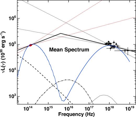
The red and black points show the mean NIR (SINFONI) and X-ray (XMM–Newton and NuSTAR) emission during the VB3 flare. The dotted red and black straight lines show the uncertainties on the determination of the NIR and X-ray power-law slope (with model BPL), respectively. The solid line shows the best-fitting PLCool model that imposes ΓX = ΓNIR + 0.5. The X-ray slope is slightly steeper (ΔΓ = 0.57 ± 0.09, 1σ), although consistent with the predictions of the PLCool model. Both X-ray and NIR data and models have been corrected for absorption and the effects of dust scattering halo. The blue solid line shows the best-fitting TSSC model (Section 5.3.3). For a description of the other lines, see Fig. 1.
4.2.2 Broken power-law model (BPL, phenomenological model)
We then performed a phenomenological description of the data with a BPL model. We observed a significant improvement and an acceptable description of the spectrum by fitting the data with this model, where the NIR and X-ray slopes were free to vary (χ2 = 154.9 for 142 dof, Δχ2 = 34.8 for the addition of 2 dof, corresponding to an F-test probability of ∼7 × 10⁻⁷; Table 5, Fig. 4). The resulting best-fitting NIR and X-ray photon indexes are ΓNIR = 1.7 ± 0.1 and ΓX = 2.27 ± 0.12, respectively (Table 5). The spectral steepening ΔΓ = 0.57 ± 0.15 (±0.09 at 1σ) is slightly steeper, but fully consistent with the value expected in the synchrotron scenario in the presence of a cooling break (ΔΓ = 0.5), strongly suggesting this latter scenario as the correct radiative mechanism.
4.2.3 Thermal synchrotron self-Compton (TSSC)
Before fitting the VB3 mean spectrum with a synchrotron model with a cooling break, we considered an alternative interpretation, where the NIR band is produced via synchrotron radiation by a thermal distribution of electrons. Moreover, the same population of electrons generates via inverse Compton the high-energy (e.g. X-ray) emission (see e.g. Dodds-Eden et al. 2011). We called this model thermal synchrotron self-Compton (TSSC). The free parameters in this model are B, the strength of the magnetic field; θE, the dimensionless electron temperature (defined as |$\theta _{\rm E}=\frac{kT_{\rm e}}{m_{\rm e} c^2}$|, where k is the Boltzmann constant, Te is the temperature of the thermal electrons, me is the electron mass and c is the speed of light); N, the total number of NIR synchrotron emitting electrons; and RF, the size of the region containing the flaring electrons, controlling the photon density of the seed photons. The very short variability time-scale (of the order of 102 s) suggests a very compact source with a size of the order of (or smaller than) a few Schwarzschild radii, likely located within or in the proximity of the hot accretion flow of Sgr A*. Radio and sub-mm observations constrain the physical parameters of the steady emission from the inner hot accretion flow (within the central ∼10RS) to be B ∼ 10–50 G, Te ∼ 1010 K, γe ∼ 10; ne ∼ 106 cm−3 (see Section 1; Loeb & Waxman 2007; Genzel et al. 2010). These are likely the pre-flare plasma conditions.
The TSSC model provides an acceptable fit to the data (χ2 = 162.7 for 139 dof; see Fig. 4).10 However, as observed in previous very bright flares (Dodds-Eden et al. 2009), the best-fitting parameters of this model are very different from the reasonable range expected to be present in the accretion flow of Sgr A*. Indeed, this model produces the flare via a magnetic field with a staggering intensity of log(B) = 4.0 ± 0.4 G, about three orders of magnitude larger than the magnetic field intensity within the steady hot accretion flow of Sgr A*, on a population of ‘not-so-energetic’ (θE = 9 ± 4) electrons. Moreover, in order to make the inverse Compton process efficient enough to be competitive to synchrotron, the electron density has to be as high as ne = 1013 cm−3, about seven orders of magnitude higher than in the accretion flow. This appears unlikely. The total number of TSSC emitting electrons is constrained by the model to be log(Ne) = 39.5 ± 0.5, therefore to reach such an excessively high electron density, the size of the emitting region has to be uncomfortably small, log(RF/RS) = −3.5 ± 0.5. Such a source would be characterized by a light crossing time of the order of only ∼10 ms. Indeed, variability on such time-scales are typically observed in accreting X-ray binaries (e.g. Belloni, Psaltis & van der Klis 2002; De Marco et al. 2015), where the system is ∼106 times more compact than in Sgr A* (Czerny et al. 2001; Gierliński, Nikołajuk & Czerny 2008; Ponti et al. 2012b), while Sgr A*'s power spectral density appears dominated by variability at much larger time-scales (Do et al. 2009; Meyer et al. 2009; Witzel et al. 2012; Hora et al. 2014).11 Again, this appears as a weakness of this model.
As already discussed in Dodds-Eden et al. (2009, 2010, 2011) and Dibi et al. (2014, 2016), these physical values are different by several orders of magnitude from the ones observed in quiescence and, therefore they appear unlikely. With this study we show that the same ‘unlikely’ physical parameters are not only observed during VB2 (the flare analysed by Dodds-Eden et al. 2009), but also during the very bright flare considered here (VB3). This confirms that this model produces unreasonable parameters for part (if not all) of the bright flares.
4.2.4 Synchrotron emission with cooling break (PLCool)
In this scenario, the synchrotron emission is produced by a non-thermal distribution of relativistic electrons, embedded in a magnetic field with strength B; therefore, they radiate synchrotron emission. At the acceleration site, the injected electrons are assumed to have a power-law distribution in γe with index p (i.e. |$N(\gamma _{\rm e})\propto \gamma _{\rm e}^{-p}$|), defined between γmin and γmax (γe being the electron Lorentz factor). We assume as lower boundary γmin = 10, supposing that the radiating electrons are accelerated from the thermal pool producing the sub-mm peak in quiescence (Narayan et al. 1998; Yuan et al. 2003). We also assume that at any point during the flare, the engine is capable of accelerating electrons to γmax > 106, so that they can produce X-ray emission via synchrotron radiation (this appears as a less reliable assumption and indeed an alternative to this scenario will be discussed in Section 8.3).
A well-known property of high-energy electrons radiating via synchrotron emission is that they cool rapidly, quickly radiating their energy on a time-scale tcool = 220(B/50 G)−3/2(ν/1014 Hz)−1/2 s (where ν is the frequency of the synchrotron emitted radiation; see Pacholczyk 1970). In particular, higher energy electrons cool faster than the NIR ones. The competition between synchrotron cooling and particle escape from the acceleration zone then generates a break in the synchrotron spectrum at a frequency: νbr = 2.56(B/30 G)−3(tesc/300 s)−2 × 10¹⁴ Hz. Furthermore, in case of continuous acceleration, a steady solution exists where the slope of the power law above the break is steeper by ΔΓ = 0.5 (Kardashev 1962) than the lower energy power law.12 Following the nomenclature of Dodds-Eden et al. (2009), we call this model ‘PLCool’. The free parameters of the PLCool model are B, p and the normalization.
As described in Section 4.2.2, a BPL model provides an excellent fit to the mean VB3 multiwavelength spectrum (χ2 = 154.9 for 140 dof). In particular, we note that the difference between the NIR and X-ray photon indices ΔΓ = 0.57 ± 0.15 (±0.09 at 1σ) is consistent with the value expected by the PLCool model (ΔΓ = 0.5; due to synchrotron emission with continuous acceleration). Indeed, imposing such spectral break (ΓX = ΓNIR + 0.5), the fit does not change significantly (χ2 = 156.8 for 141 dof), with the photon index ΓNIR = 1.74 ± 0.08 and the break at |$0.04^{+0.12}_{-0.03}$| keV (|$B=8.8^{+5.0}_{-3.0}$| G; Fig. 4). We note that the PLCool model provides a significantly better fit (χ2 = 156.8) than the TSSC model (χ2 = 161.3) despite having two fewer free parameters (Table 5).
To investigate the effects of potential uncertainties on the normalization of the NIR emission, we artificially increased (and decreased) the SINFONI spectrum by a factor 1.25 (and 0.75). The statistical quality of the fit does not change (χ2 = 156.8 for 141 dof, in all cases), and neither does the best-fitting photon index, ΓNIR = 1.74 ± 0.08. As expected, the main effect of the higher (lower) NIR normalization is to shift the break towards lower (higher) energies, i.e. |$E_{\text{br}}=0.018^{+0.071}_{-0.014}$| keV (|$E_{\text{br}}=0.046^{+0.20}_{-0.037}$| keV), corresponding to |$B=11.7^{+8.5}_{-3.3}$| G (|$B=8.5^{+5.5}_{-3.0}$| G).
5 EVOLUTION DURING VB3
5.1 Light curves of VB3
The black and red points in Fig. 5 show XMM–Newton and NuSTAR light curves of VB3 in the 2–10 and 3–20 keV bands, respectively. The black dashed line indicates the level of diffuse and quiescent emission observed by XMM–Newton. For display purposes, we subtracted a constant rate of 0.13 cts s−1 from the NuSTAR light curve, to take into account the different contribution of the diffuse and quiescent emission. The squares in Fig. 5 show the NIR light curve as observed with SINFONI. Despite the sparse sampling of the light curve allowed by the SINFONI integral-field unit, it is clear from Fig. 5 that for VB3 the NIR flare lasts longer than the X-ray one. In particular, the NIR flare is already in progress during our first SINFONI integration, ∼103 s before the start of the X-ray flare and it is still in progress at the end of IR4, with a duration longer than 3.4 ks (see Fig. 5, Tables 1 and 3). This is not surprising, indeed, a similar trend has already been observed by Dodds-Eden et al. (2009) and Trap et al. (2011) in the only other very bright flare with simultaneous NIR coverage (see fig. 3 of Dodds-Eden et al. 2009). The pink dashed lines in Fig. 5 indicate the start and end of the XMM–Newton VB3 flare as determined by the Bayesian block decomposition (see Ponti et al. 2015c). The dotted green lines indicate the periods during which VB3-Pre, VB3-Rise, VB3-Peak, VB3-Dec and VB3-Post have been integrated (Table 1).
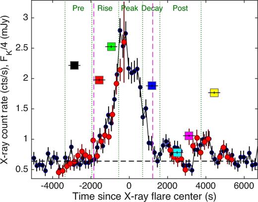
The black and red points show the XMM–Newton 2–10 keV (sum of the three EPIC cameras) and NuSTAR 3–20 keV light curve of Sgr A*'s flare VB3 (Ponti et al. 2015c), respectively. A constant rate of 0.13 cts s−1 has been subtracted from the NuSTAR light curve for display purposes, to take into account the different contribution of the diffuse and quiescent emission (gaps in the NuSTAR light curve are due to Earth occultation). The squares show the extinction corrected SINFONI light curve of Sgr A* during the VB3 flare. Each point corresponds to an NIR spectrum integration time of 600 s. The y-axis reports the observed renormalized (divided by 4 for display purposes) flux density at 2.2 μm in mJy units. The black dashed line indicates the level of the ‘non-flare’ (quiescent in X-rays) emission. The pink dashed lines indicate the start and end of the XMM–Newton VB3 flare, as indicated by the Bayesian block decomposition (see Ponti et al. 2015c). Excess X-ray emission is observed ∼2000 and ∼4000 s after the X-ray flare peak. The dotted green lines show the intervals for the integration of the pre-, rise, peak, decrease and post-flare spectra during VB3. The zero-point of the abscissa corresponds to 525831144.7 s (TTTBD) and 2456900.50784 d (BJDTBD), respectively.
The second and third column show the Barycentre corrected start and end times of each of the seven SINFONI spectra. Times are Barycentric Julian Dates in Barycentric Dynamical Time. The last two columns show the test fit photon index (Γ) and flux once the SINFONI data are fitted with a simple power-law model.
| Spec | tstart | tstop | Γ | |${F_{2.2\mu \text{m}}}^a$| |
|---|---|---|---|---|
| BJDTBD | BJDTDB | (mJy) | ||
| IR1 | 2456900.47470 | 2456900.48164 | 1.48 ± 0.23 | 8.87 ± 0.10 |
| IR2 | 2456900.48971 | 2456900.49665 | 1.37 ± 0.19 | 7.91 ± 0.07 |
| IR3 | 2456900.49694 | 2456900.50388 | 1.80 ± 0.13 | 10.09 ± 0.07 |
| IR4 | 2456900.52160 | 2456900.52855 | 1.76 ± 0.21 | 7.52 ± 0.06 |
| IR5 | 2456900.53675 | 2456900.54370 | 3.71 ± 0.48 | 3.12 ± 0.07 |
| IR6 | 2456900.54398 | 2456900.55093 | 2.72 ± 0.23 | 4.23 ± 0.04 |
| IR7 | 2456900.55914 | 2456900.56608 | 2.56 ± 0.21 | 7.07 ± 0.06 |
aThe error bars are statistical only and they do not include systematic effects due to spectral extraction. The effect of systematics is treated in Section 5.3.4.
Best-fitting parameters of the fit of the very bright flares of Sgr A*. Column densities are given in units of 1023 cm−2 and the absorbed fluxes are in units of 10−12 erg cm−2 s−1.
| Absorbed power-law fit to X-ray spectra | ||||
|---|---|---|---|---|
| Name | NH | ΓX | Flux2–10 | χ2/dof |
| VB1 | 1.6 ± 0.2 | 2.2 ± 0.3 | |$9.6^{+7}_{-4}$| | 89.9/114 |
| VB2 | 1.6 ± 0.3 | 2.3 ± 0.4 | |$5.0^{+5}_{-2.4}$| | 89.3/98 |
| VB3 | 1.6 ± 0.3 | 2.3 ± 0.3 | |$7.6^{+7.1}_{-3.4}$| | 127.2/117 |
| VB123a | 1.59 ± 0.15 | 2.20 ± 0.15 | 302.8/331 | |
| VB123|$_{\text{Fix}N_{\text{H}}}{}^b$| | 1.6 | 2.21 ± 0.09 | 302.8/332 | |
| VB3XMM+Nub | 1.6 | 2.27 ± 0.12 | 7.5 ± 1.5 | 141.4/133 |
aThe VB123 flare indicates the average of VB1+VB2+VB3.
bThe VB123|$_{\text{Fix}N_{\text{H}}}$| shows the best-fitting results of flare VB123, once the column density of neutral absorbing material has been fixed. The VB3XMM+Nu shows the best-fitting results of flare VB3 (by fitting both XMM–Newton and NuSTAR data), once the column density has been fixed.
Best-fitting parameters of the mean spectrum of VB3 with the single PL (plain synchrotron), BPL, TSSC and PLCool (power-law cool) models. See Section 4 for a description of the parameters.
| VB3 mean spectrum | ||||
|---|---|---|---|---|
| Single PL | BPL | TSSC | PLCool | |
| ΓNIR | 2.001 ± 0.005 | 1.7 ± 0.1 | 1.74 ± 0.08 | |
| ΓX | 2.27 ± 0.12 | |||
| ΔΓ | 0.57 ± 0.15 | 0.5 | ||
| log(B) | 0.94 ± 0.16 | 4.0 ± 0.4 | 0.94 ± 0.16 | |
| Θe | 9 ± 4 | |||
| log(Ne) | 39.5 ± 0.5 | |||
| log(RF) | −3.5 ± 0.5 | |||
| χ2/dof | 189.7/142 | 154.9/140 | 162.7/139 | 156.8/141 |
5.2 NIR spectral evolution during VB3
We fit all the seven high quality SINFONI spectra (see top panel of Fig. 6) with a simple power-law model, normalized at 2.2 μm (pegpwrlw). The fit with this simple model provides a χ2 = 96.8 for 56 dof. The bottom panel of Fig. 6 shows the best-fitting photon index (ΓNIR, where Γ = 1 − α and α is the spectral index Fν ∝ να) as a function of the flux density (in mJy) at 2.2 μm.
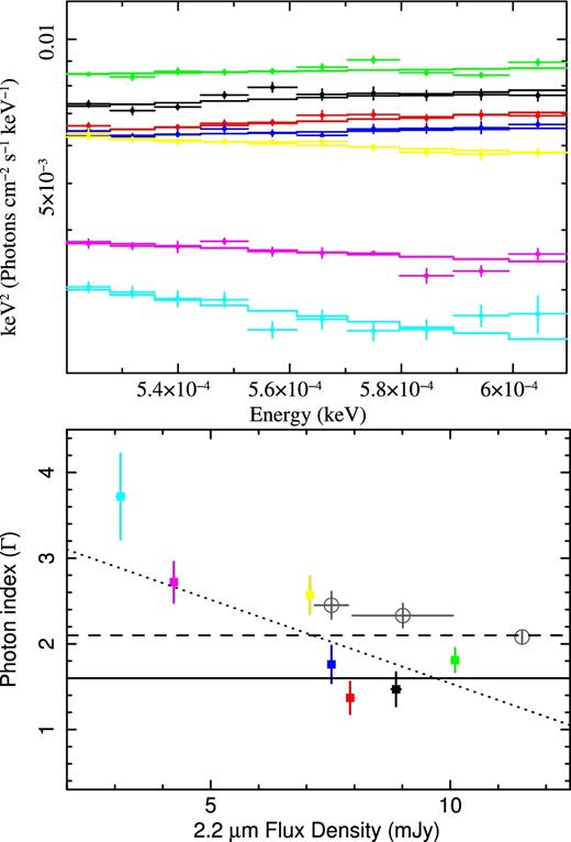
(Top panel) SINFONI spectra fitted with a power-law model in the energy band E ∼ 0.525–0.608 eV. The colour (black, red, green, blue, cyan, magenta and yellow) indicates the chronological sequence of the spectra. (Bottom panel) Best-fitting photon index (ΓNIR) as a function of the 2.2 μm flux density (in mJy units). The NIR photon indexes are shown with filled squares, with the same colour code as before. The empty dark grey circles show the spectral indexes in the 2–10 keV band, during the rise, decay and peak of very bright flares. For these points, we associate to the flare rise and decay X-ray photon indexes the simultaneous NIR fluxes. For the flare peak, we assume a value of 11.5 mJy. The dotted lines show the best fit of the NIR photon indexes with a linear relation. The solid line shows the constant photon index typically observed at medium-high fluxes (flux density >7 mJy; ΓNIR = 1.6; Hornstein et al. 2007). The dashed line shows the associated X-ray slope, if the spectrum is dominated by synchrotron emission with a cooling break ΓX = ΓNIR + 0.5.
During the SINFONI observations the 2.2 μm flux density ranges from ∼3 to ∼10 mJy, spanning the range between a classical dim and bright NIR period (Bremer et al. 2011). This suggests that this very bright X-ray flare is associated with a very bright NIR flux excursion. In agreement with previous results, we observe a photon index consistent with ΓNIR = 1.6 above ∼7 mJy (solid line in Fig. 6; Hornstein et al. 2007; Witzel et al. 2014). On the other hand, Fig. 6 also shows steeper NIR spectral slopes at low fluxes. We note that steep NIR slopes at low fluxes have been already reported (Eisenhauer et al. 2005; Gillessen et al. 2006; Bremer et al. 2011); however, recent observations by Witzel et al. (2014) indicate no spectral steepening at low fluxes. The results of our work appear to suggest an evolution of the spectral slope at low fluxes during and after this very bright X-ray flare; however, higher quality data are necessary to finally clarify this trend.
5.3 Multiwavelength spectral evolution during VB3
We extracted strictly simultaneous XMM–Newton and NuSTAR spectra for each of the seven NIR SINFONI spectra (see Fig. 10). All are covered by XMM–Newton and NuSTAR, apart from spectrum IR4, for which Sgr A* was not visible by NuSTAR at that time (due to Earth occultation). The first four (from IR1 to IR4) of these spectra have been accumulated either when the X-ray counterpart of VB3 was visible or in their close proximity and they all show bright NIR emission; therefore, we present the results of the analysis of those ‘flaring spectra’ here. The remaining three, associated with faint NIR and X-ray quiescent emission, are investigated in the next section (Section 6).
We stress again that during the IR1 spectrum the flare was already very bright (|$F_{2.2\,\mu \text{m}}\sim 9$| mJy) in the NIR band, while only upper limits were observed in X-rays (see Figs 5 and 7). Indeed, the X-ray flare started roughly 20 min later, during IR2, and peaked just after IR3. Bright NIR emission with no X-ray counterpart in the early phases of the flare places tight constraints on the PLCool model (see Section 8). During IR4 the NIR flux was still high (|$F_{2.2\mu \text{m}}\sim 7.5$| mJy), while the X-ray flare was about to end (Fig. 5). After IR4 the NIR dropped significantly and the X-ray emission returned to the quiescent level.
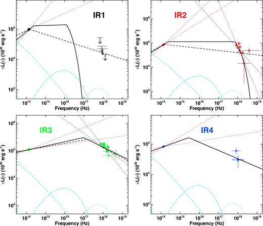
Evolution of Sgr A*'s SED during the very bright flare VB3. Each panel shows the SINFONI and simultaneous X-ray spectra fitted with the PLCool model, during each of the four SINFONI spectra integrated during the VB3 flare (see Fig. 5). The colour code is the same as in Fig. 5, with the temporal sequence: black; red; green and blue. The red and black dotted lines show the uncertainties in the determination of the NIR and X-ray power-law slopes, respectively. The X-ray slopes are well determined only for the IR2 and IR3 spectra. The black dashed lines show the best-fitting PLCool models, where ΓX = ΓNIR + 0.5 is imposed. For IR2, the observed X-ray slope is inconsistent with the predictions of the PLCool model. For both IR1 and IR2, the cooling break is suspiciously pegged in the NIR band. The black solid lines show the best-fitting PLCoolEv models. During IR1, both the cooling break and the cut-off have large uncertainties, but are constrained to lie within few 1014 < ν < 1018 Hz. During IR2, the cut-off is in the X-ray band. From IR2 to IR3 the cooling break evolves to higher energies and then back to lower energies during IR4. Sgr A* is undetected in X-rays during observation IR1. Such as in Fig. 4 both data and models are de-absorbed and corrected for the effects of the dust scattering halo. For a description of the other lines, see Fig. 1.
5.4 Is the spectral evolution required?
We started the time-resolved spectral analysis by testing whether the data require any spectral evolution during VB3. We therefore simultaneously fitted the multiwavelength flaring spectra (IR1, IR2, IR3 and IR4) with a BPL model, forcing the NIR and X-ray photon indexes and the break energy to be constant over time. This provides an unacceptable fit (χ2 = 237.6 for 104 dof), demonstrating that significant spectral variability is required during the flare. The best-fitting photon indexes are ΓNIR = 1.71 ± 0.09, ΓX = 2.21 ± 0.10, with the break at |$E_{\text{br}}=10^{+150}_{-3}$| eV. We note that, similar to what has been found in the analysis of the mean spectrum, the spectral steepening is ΔΓ = 0.50 ± 0.13, therefore perfectly consistent with ΔΓ = 0.5.
We then refitted the spectra with the same model, allowing the NIR photon index and the break energy to evolve with time, while imposing the X-ray photon index to be ΓX = ΓNIR + 0.5. This provided a significant improvement to the fit (Δχ2 = 97.6 for the addition of five new parameters), demonstrating that Sgr A*'s spectrum changed shape during VB3. Indeed, we observe best-fitting photon indexes of ΓNIR1 = 1.70 ± 0.05, ΓNIR2 = 1.60 ± 0.08, ΓNIR3 = 1.91 ± 0.07 and ΓNIR4 = 1.81 ± 0.13, while the break is at Ebr1 = 0.6 ± 0.03, Ebr2 = 0.9 ± 0.03, |$E_{\text{br}3}=1150^{+1800}_{-800}$| and |$E_{\text{br}4}=14^{+400}_{-11}$| eV. We note that this model can acceptably reproduce the data (χ2 = 140.0 for 99 dof).
5.5 Evolution of the BPL model during VB3
Before considering the PLCool model, where the slopes in NIR and X-rays are tied by the relation ΓX = ΓNIR + 0.5, we fitted each time-resolved multiwavelength spectrum with the phenomenological BPL model (Section 4.2.2), where the slopes in the NIR and X-ray bands are free to vary (Table 6).
Best-fitting parameters of Sgr A*'s emission as fitted during each of the (600 s) SINFONI and strictly simultaneous X-ray spectra accumulated during the flare VB3. The spectra are fitted with the BPL, the PLCool and the PLCoolEv models. ΓNIR and ΓX indicate the power-law photon indexes fitting the NIR, the X-ray band, respectively. For the PLCool and PLCoolEv models, the ΓNIR indicates the best-fitting NIR slope, once the total band is fitted with the assumption that ΓX = ΓNIR + 0.5. Ebr indicates the energy of the cooling break. Ec indicates the energy of the high-energy cut-off (induced by γmax).
| Simultaneous (600 s) NIR to X-ray spectra during VB3 | ||||
|---|---|---|---|---|
| BPL | ||||
| ΓNIR | ΓX | Ebr | χ2/dof | |
| (eV) | ||||
| IR1 | 1.5 ± 0.2 | >2.2 | 1b | 20.8/15 |
| IR2 | 1.4 ± 0.2 | 3.2 ± 0.4 | |$0.16^{+0.20}_{-0.11}$| | 32.8/24 |
| IR3 | 1.8 ± 0.2 | 2.57 ± 0.16 | |$420^{+980}_{-210}$| | 43.8/43 |
| IR4 | 1.8 ± 0.2 | 2.14 ± 0.02 | 1b | 11.4/10 |
| PLCool | ||||
| ΓNIR | Ebr | χ2/dof | ||
| (eV) | ||||
| IR1 | 1.72 ± 0.04 | 0.60 ± 0.03a | 23.7/15 | |
| IR2 | 1.58 ± 0.01 | 0.61 ± 0.03a | 43.8/25 | |
| IR3 | 1.87 ± 0.07 | |$530^{+1400}_{-380}$| | 46.0/44 | |
| IR4 | |$1.77^{+0.06}_{-0.02}$| | |$9.7^{+77}_{-8.0}$| | 11.2/10 | |
| PLCoolEv | ||||
| ΓNIR | Ec | Ebr | χ2/dof | |
| (keV) | (eV) | |||
| IR1 | |$1.48^{+0.25}_{-0.05}$| | 6 × 10⁻⁴ to 1 | 0.6–1000 | 17.4/14 |
| IR2 | 1.5 ± 0.2 | |$3.5^{+0.3}_{-1.1}$| | |$1^{+2}_{-0.5}$| | 35.6/24 |
| IR3 | 1.82 ± 0.07 | >9 | |$250^{+780}_{-150}$| | 45.3/43 |
| IR4 | |$1.77^{+0.06}_{-0.02}$| | >10 | |$9.8^{+77}_{-8.3}$| | 11.0/9 |
aThe best-fitting energy of the break falls right at the higher edge of the SINFONI energy band.
bUnconstrained value, therefore fixed to 1 eV.
The NIR slope was always well determined (ΔΓNIR ∼ 0.2; see Tables 3 and 6). On the other hand, the presence of either upper limits or low statistics prevented us from determining ΓX at the same time of Ebr in spectra IR1 and IR4 (Table 6). We, therefore, ‘a priori’ assumed that the breaks in IR1 and IR4 occur at 1 eV (which corresponds to B = 30 G, if interpreted as a cooling break). We then constrained the power-law slopes in the X-ray band under this assumption (ΓX > 2.2 and ΓX = 2.14 ± 0.02 for IR1 and IR4, respectively). Moving the break to 25 eV (corresponding to B = 10 G) the slope would steepen to ΓX > 2.6 and ΓX = 2.4 ± 0.1, respectively. For IR2 and IR3, the X-ray data are of good enough quality to have a good constraint on the X-ray slope (see Table 6). The dotted lines in the corresponding panels of Fig. 7 show the uncertainties on the X-ray and NIR slopes. The BPL model produced an acceptable description of the spectra (the surviving residuals are due to intrinsic scatter in the NIR band; see Table 6).
5.6 Evolution of the PLCool model during VB3
We then fitted the spectra with the PLCool model (Fig. 7; Table 6). This model reproduces synchrotron emission with a cooling break under the assumption that, at any time, γmax > 106.
5.6.1 Successes of the PLCool model
For IR1, IR3 and IR4, the PLCool model provides a good fit to the data of indistinguishable (at 90 per cent confidence) quality compared to the phenomenological BPL model (Table 6). The advantage over BPL is that the PLCool model is physically motivated.
We observed that for all spectra (from IR1 to IR4) the NIR spectra are flat and consistent with being constant (e.g. ΓNIR ∼ 1.6, see Fig. 6) before and during the full duration of the X-ray flare. This is in line with the values typically observed during bright NIR flux excursions (Hornstein et al. 2007).13 We also noted that at the peak of the X-ray flare, when the constraints are best, the X-ray slope is steeper than the simultaneous NIR one by ΔΓ ∼ 0.5, consistent with the one expected by the PLCool model (see Fig. 7 and Table 6).
Blindly applying the PLCool model to all time-resolved spectra (it might be incorrect to apply the PLCool model when no X-ray emission is detected), we observed a significant evolution of the energy of the cooling break, that implies (under the assumption of a constant escape time) a variation of the strength of the magnetic field (Table 6). The black, red, green, blue and grey dotted and solid lines in Fig. 8 show the 68 and 90 per cent confidence contours of the uncertainty on Ebr and ΓIR for IR1, IR2, IR3, IR4 and the mean spectrum, respectively. We note that a highly significant evolution of the cooling break is observed. Indeed, during both IR1 and IR2, the break appears to be at very low energy, corresponding to a magnetic field of the order of B ∼ 35 G. While the energy of the break is significantly higher during IR3, indicating that the magnetic field had significantly reduced around the peak of the X-ray flare (|$B=3.8^{+2.0}_{-1.3}$| G). The energy of the break then drops again in the decreasing flank of the X-ray flare to a value of |$E_{\text{br}}=9.7^{+77}_{-8.0}$| eV, corresponding to an increase in the strength of the magnetic field (|$B=14.3^{+11.3}_{-7.4}$| G).
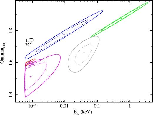
The black, red, green, blue and grey lines show confidence contours of the uncertainty on Ebr and ΓIR for IR1, IR2, IR3, IR4 and the mean spectrum once fitted with the PLCool model, respectively. The dotted and solid lines show the 68 and 90 per cent confidence contours, respectively. During IR1 and IR2 the cooling break pegs at its lowest value, being located just above the NIR band. Once fitted with the PLCoolEv model, the confidence contours remain unchanged for IR3, IR4 and the mean spectrum, because during these intervals the high-energy cut-off is at very high energy. The magenta lines show the confidence contours during IR2, when the cut-off is observed in the X-ray band. During IR1, the cut-off falls between the NIR and X-ray band, therefore the location of the cooling break is unconstrained.
5.6.2 Difficulties of the PLCool model
As we have outlined, the PLCool model (which assumes γmax > 106 at all times) presented many successes. However, we also point out here three severe weaknesses that will be discussed further in the discussion section: (i) twice out of four times the cooling break is observed to peg just above the NIR band (E ∼ 0.6 eV). This appears as a rather unlikely possibility; (ii) during IR1, bright and flat (Γ = 1.48 ± 0.2) NIR emission is associated to no enhanced X-ray emission (F3−10keV < 2.3 × 10⁻¹² erg cm−2 s−1). This is hard to reconcile with the PLCool model that, in order to fit this spectrum, pushes the best-fitting NIR photon index to ΓNIR = 1.72 ± 0.04; (iii) the very steep X-ray spectrum during IR2 (ΓX = 3.2 ± 0.4) implies a spectral steepening incompatible with the PLCool model (ΔΓ = 1.8 ± 0.4, instead of ΔΓ = 0.5).
5.7 Can the TSSC model fit the IR2 spectrum?
In theory, SSC models, with a thermal distribution, can produce fairly steep spectral shapes at high energies. Therefore, although the TSSC model produced unreasonable parameter values when applied to the mean VB3 spectrum, we checked whether TSSC might be the dominant radiative mechanism during peculiar and short duration intervals, such as IR2.
The best-fitting TSSC model was significantly worse than the PLCool model, despite having two more free parameters (χ2 = 60.1 for 23 dof). Indeed, the model failed to produce a better fit because it was mainly constrained by the flat X-ray photon index produced by the TSSC model. In addition, we noted that the fit of IR2 leaded to unreasonable best-fitting parameters, similar to the ones fitting the mean VB3 spectrum. Indeed, we observed: log(B) = 3.55, θE = 32.6, log(Ne) = 39.3 and log(RF/RS) = −3.0. Once again the magnetic field strength appears, unreasonably large, the size of the source unreasonably small, and the source density many orders of magnitude higher than expected.
5.8 Synchrotron emission with cooling break and evolving γmax (PLCoolEv)
When we considered the PLCool model, we ‘a priori’ used the assumption that at any time the source can accelerate particles to very high energies γmax > 106. This implies that an engine, able to accelerate electrons to γmax > 106, is created on a negligible time-scale, at the start of the NIR flare. If so, the PLCool model can be applied to the entire duration of the flare (as we performed in Section 5.6.2).
On the other hand, if the engine has a size of a few Schwarzschild radii, its light (or Alfvén speed) crossing time would be of the order of a hundred seconds, comparable to the time-scales of the flares under investigation here. Thus, it might be possible that the creation and destruction of the engine occurs on a similar time-scale to the flares and that the engine is initially not powerful enough to accelerate particles to γmax > 106. Based on these considerations, we introduce a new phenomenological model dubbed PLCoolEv, by adding to the PLCool model the freedom of having a variable value of γmax. We performed this by adding a high-energy cut-off to the PLCool model (reproduced by the highecut component in xspec). Indeed, the PLCoolEv model assumes that γmax evolves during the flare. A low value of γmax (e.g. γmax ≪ 106) would imply that no electrons are accelerated to such high energies to produce X-ray photons.14 As a result, the emitted spectrum would show a high-energy cut-off (Ec) at an energy related to γmax and lower than the X-ray band. As in the PLCool model (with free parameters: B, p and normalization), this model is characterized by the cooling break Ebr, linked to the strength of the magnetic field, plus a cut-off at high energy Ec (induced by γmax).
We assumed an exponential shape above the cut-off energy. We noted that such shape is constrained only by the IR2 spectrum and it appears steeper (ΓX = 3.2 ± 0.4) than the simultaneous and cooled NIR slope (see Table 6). Therefore, any high-energy slope steeper than ΓX ∼ 3 could reproduce the data. We point out that either an exponential or sub-exponential slope can equally fit the data. We also note that most likely the electron distribution will not cut abruptly at γmax; therefore, it is expected that the cut-off will be further broadened. Despite we could not constrain whether the break is broad, we fixed the shape of the high-energy cut-off such that the e-folding energy of the exponential cut-off is equal to the cut-off energy.
The PLCoolEv model provides an excellent representation of the multiwavelength spectrum at all times during the flare (see Table 6 and Fig. 7). It produces either superior fits compared to PLCool model (in particular for IR2), or of comparable statistical quality to the BPL parametrization and it is physically motivated.
Fig. 8 shows the confidence contours projected over the Ebr versus ΓNIR plane for the PLCoolEv model. The high-energy cut-off is constrained to be at 7 × 10⁻⁴ < Ec < 1 keV in the IR1 spectrum, before the start of the X-ray flare (not shown in Fig. 8). In the PLCool model, the steep photon index observed in X-ray during IR2 is the result of the evolution of the high-energy cut-off, which at that time was detected in the X-ray band at |$E_{\rm c}=3.5^{+0.3}_{-1.1}$| keV. As a consequence of this, the cooling break is not pegged anymore at Ebr = 0.6 eV, instead it spans a larger range of reasonable cooling break energies. Additionally, a flatter NIR slope is allowed. During IR3, IR4 and the mean spectrum, the high-energy cut-off was at energies higher than the observed X-ray band (Ec ≫ 10 keV), consistent with the assumptions of the PLCool model (indeed, we obtained similar results). According to the PLCoolEv model, during the early phase of VB3, the high-energy cut-off was evolving and it was located between the NIR and X-ray band. It was caught within the X-ray band during IR2 and it was at very high energy at the X-ray peak (and during IR4).
5.8.1 Evolution of the magnetic field (assuming a constant escape time)
In this section, we interpret the derived evolution of the energy of the cooling break, as being uniquely due to the variation of the magnetic field of the source (e.g. assuming no variation of the escape time).
Fig. 9 shows the light curve of the evolution of the magnetic field intensity during the flare. The flat NIR slope observed at all times indicated that the break has to be, at higher frequency compared to the SINFONI band, corresponding to B < 36 G. In particular, during IR2 the cooling break is observed at |$E_{\text{br}}=1^{+2}_{-0.5}$| eV, corresponding to B = 30 ± 8 G. The values derived by fitting the IR1 spectrum are consistent with this value, however the degeneracy between the energy of the cooling break and of the high-energy cut-off led to large uncertainties on the magnetic field strength. We note that a value of B = 30 ± 8 G is fully consistent with the magnetic field present within the central ten Schwarzschild radii and generating the steady emission of Sgr A*. During IR3, close to the peak of the X-ray flare, the magnetic field is observed to be B = 4.8 ± 1.7 G. Interestingly, the magnetic field varied by a factor of >6 in less than ∼650 s. During IR4, we assumed that the cut-off is located at energies higher than the X-ray band (indeed no evidence for a cut-off at or below the X-ray band is observed). Under this assumption,15 we observe that after the X-ray peak and towards the end of the X-ray flare, the magnetic field was measured to rise again to values |$B=14.3^{+12.3}_{-7.0}$| G. The red point in Fig. 9 shows the magnetic field strength derived from the fit of the mean spectrum of VB3. As expected, the average magnetic field value during the flare (|$B=8.8^{+5.0}_{-3.0}$| G) was intermediate between IR2, IR3 and IR4 and it was significantly smaller than the one derived during quiescence.
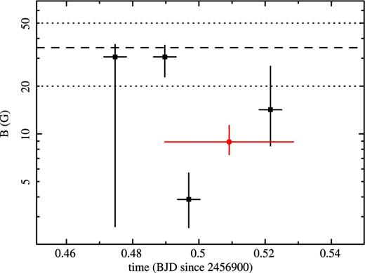
Evolution of the strength of the magnetic field (in Gauss) during and after the flare VB3, in the PLCoolEv model. The black square shows the magnetic field strength during IR1 to IR4. The red circle shows the measurement of the average magnetic field during the entire duration of the X-ray flare VB3 (under the assumption of a constant escape time of tesc = 300 s). The dotted lines indicate the typical range of magnetic field strengths during quiescence (B ∼ 20–50 G). The dashed line shows the magnetic field strength (B ∼ 36 G) corresponding to a cooling break within the narrow SINFONI band. The flat NIR slopes observed at all times during the flare suggest B < 36 G, while the steep NIR slope observed after the VB3 flare (during IR5, IR6 and IR7) suggest B > 36 G. The error bars correspond to the 1σ uncertainties as derived from the confidence contours shown in Fig. 8. No evidence for a cut-off at or below the X-ray band is observed during IR4, therefore the associated measurement is valid under the assumption that the cut-off is at energies higher than the X-ray band. Would this assumption be invalid, such constraint should be considered as an upper limit.
5.8.2 Evolution of the escape velocity (constant magnetic field)
The results obtained in Section 5.8.1 are valid under the assumption that the synchrotron escape time is constant over the entire duration of the flare. However, it is not a priori set that the escape time has to remain constant over time. Therefore, we now investigate the hypothesis that the escape time evolves, while assuming a constant magnetic field (B = 30 G). If so, the energies of the break frequencies observed during IR2, IR3 and IR4 (|$E_{\text{br}}=1^{+2}_{-0.5}$|, |$250^{+780}_{-150}$| and |$9.8^{+77}_{-8.3}$| eV) correspond to an escape velocity of tesc1 = 310 ± 130 s, tesc2 = 20 ± 10 s and |$t_{\text{esc}3}=100^{+150}_{-70}$| s. Therefore, the escape time would drop by a factor of ∼16 in ∼600 s, to then increase again.
The escape time is likely related to the source size and/or to the position of the source on to the accretion disc. For example, Dodds-Eden et al. (2009) assume that the escape time is comparable to the dynamical time at a given radius in an accretion disc (tdyn): |$t_{\text{esc}}\sim t_{\text{dyn}} = \sqrt{R^3/2GM_{\text{BH}}}$|, where R is the source position within the accretion disc, G is the gravitational constant and MBH is the BH mass. We note that, under this assumption, the escape time assumed throughout the paper (tesc = 300 s) corresponds to a reasonable radial position of ∼3.5RS from the BH.
In summary, the PLCoolEv can adequately fit not only the mean properties of the VB3 flare but also its evolution. The major weaknesses of the PLCool model are solved by allowing the high-energy cut-off (γmax) to evolve during the flare.
We note that the evolution of the cooling break appears more likely induced by a variation of the magnetic field that drops its intensity by discharging magnetic energy density into particle acceleration and then rises again to its average value, compared to a variation of the escape velocity. Indeed, in the latter scenario it would naively be expected that the energy release produced by the source would make the source size expand with time, instead of contracting. However, we point out that these considerations are not conclusive. Indeed, because of the limitations of our simplified single zone models, we cannot discriminate between a pure magnetic field evolution or a pure escape time evolution (or a combination of both).
6 EMISSION AFTER VB3 (X-RAY QUIESCENCE)
IR5 and IR6 have been accumulated after the end of VB3 when only upper limits are observed in X-rays and the NIR flux (|$F_{2.2\mu \text{m}}\le 4.5$| mJy) corresponds to the faintest fluxes of Sgr A*, detected so far (e.g. Dodds-Eden et al. 2010). These time intervals appear similar to classical quiescent periods. During IR7 a re-brightening is observed in NIR, associated with a hint for an excess in the X-ray band (Fig. 5). Though the NIR flux is relatively high (|$F_{2.2\mu \text{m}}\sim 7$| mJy), the NIR spectral slope appears steeper than during the flare and fully consistent with the value observed during NIR quiescence. The sparse NIR light curve as well as the low significance of the X-ray excess do not allow us to clarify whether the emission during IR7 is produced by a faint flare, with associated feeble X-ray emission or it is just an NIR fluctuation characteristic of a red noise process, commonly occurring during X-ray quiescence.
We observed that the NIR spectra steepened ∼15 min after the end of the X-ray flare (see Table 3). The steepening was so large (ΔΓNIR ∼ 1–2) that in all cases (from IR5 to IR7) the extrapolation of the steep power law observed in the SINFONI band (Table 3) was consistent with the X-ray upper limits. Fig. 6 shows that at medium-high NIR fluxes (|$F_{2.2 \mu \text{m}}>7$| mJy) the photon index is consistent with a constant value of ΓNIR = 1.6. This implies an electron distribution index of p ∼ 2.2. We note that in the PLCool (and PLCoolEv) model, as long as B > 35–40 G, the cooling break would move to frequencies lower than the SINFONI band, inducing a steepening of the observed photon index by ΔΓNIR = 0.5. However, this steepening appears too small to reproduce the full extent of the observed photon index variation. We remind the reader that accurate photon index determination at low NIR fluxes are challenging. Therefore, we leave to future dedicated studies to establish the full extent and the reliability of the NIR spectral steepening at low NIR fluxes. If future data confirms the presence of such steep NIR slopes after very bright flares, then this radiation might be associated with thermal Synchrotron emission from electrons transiently heated during VB3. Indeed, we note that, for a magnetic field strength of B ∼ 30 G, the cooling time of NIR synchrotron electrons is of the order of ∼500 s, shorter, but comparable, to the time interval between the end of IR4 and the start of IR5 (see Fig. 5 and Table 3).
7 Does a slow evolution of γmax agree with the evolution of bright X-ray flares?
The detailed investigation of the X-ray and NIR emission during VB3 indicates the PLCoolEv as the favourite model (see Sections 5 and 6). The essential component that distinguish the PLCoolEv model from the simpler PLCool model is the evolution of the cut-off (γmax). In particular, we suggest that the evolution of γmax might be relatively slow, spanning the range from optical–NIR to X-rays and beyond on macroscopic time-scales (∼102–103 s). We also note that the X-ray band has significant extensions in frequency, spanning over a decade in frequency. Therefore, should the PLCoolEv model be correct and should the behaviour observed during the very bright flare VB3 be universal, then this model would predict an energy dependent evolution of X-ray flares that might be tested with archival data of other bright X-ray flares.
Indeed, it is expected that the passage of the cut-off (induced by γmax) through the X-ray band would induce slightly shorter flares at higher energies as well as steeper spectral slopes at the start and end of the X-ray flare. Clearly the full extent of these effects cannot be predicted, because it depends on how rapidly the cut-off spans the X-ray band, but we investigated whether we can exclude that such evolution is present during bright X-ray flares. Indeed, despite the fact that at present there are only few bright and very bright flares with multiwavelength coverage and only one (VB3) with simultaneous NIR and X-ray spectra, the XMM–Newton archive contains several bright flares suitable for studying the spectral evolution in the X-ray band.16
7.1 Time dependence of X-ray spectra of very bright flares
To follow the evolution of Sgr A*'s X-ray emission during very bright X-ray flares, we consider here all bright and very bright flares observed by XMM–Newton (see Table 1; Ponti et al. 2015c). For each of these flares we extract three spectra, one during the rise, one at the peak and one during the decay (see Table 1).17 We fit the spectra from both the EPIC-pn and EPIC-MOS data during the peak of VB1, VB2 and VB3 with the absorbed power-law model. The observed spectral indices at peak are consistent between the different flares; therefore, we assume the same value and redo the fit to obtain a best-fitting value of Γ = 2.08 ± 0.11 (±0.07 at 1σ). We then repeat this exercise fitting the spectra during both the flare rise and decay, obtaining Γ = 2.33 ± 0.23 and Γ = 2.45 ± 0.25, respectively. Again, we observe consistent values for the rises and decays of different flares. Therefore, we assume the same spectral index during both flanks of the flares, obtaining a best-fitting value of Γ = 2.36 ± 0.15 (±0.09 at 1σ), slightly steeper (∼2.4σ significance) than the spectral index observed at peak. We conclude that the spectra of very bright flares provide hints for (or at least are not in disagreement with) an evolution of the order of ΔΓ ∼ 0.3 between the peak and the flanks of the flares. This behaviour is reminiscent of what was observed during the evolution of VB3. Indeed, during the early phases of the X-ray emission (IR2), the X-ray spectrum was steeper than at the peak of the X-ray emission (IR3; Section 5), most likely because of the evolution of γmax.
7.2 Colour dependence of bright X-ray flares
Fig. 10 shows the 2–10 keV band light curves of the three very bright flares observed by XMM–Newton (Ponti et al. 2015c). We combined the light curves from the three EPIC cameras. Fig. 10 shows a remarkable similarity in the evolution of these flares, suggesting an analogous origin. We fit each of the light curves with a model composed by a constant plus a Gaussian profile (to fit the flare).18
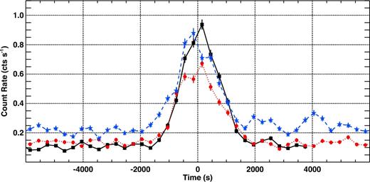
Light curves, in the 2–10 keV band, of the three brightest XMM–Newton flares, VB1, VB2 and VB3 are shown with back squares, red circles and blue stars, respectively. The light curves of the three very bright flares observed by XMM–Newton show very similar time evolution and comparable duration. These light curves are the result of the sum of the data from EPIC-pn and EPIC-MOS. For display purposes, we shifted the time axis aligning the peak of the Gaussian best fitting the flare profile (see Table 7).
To investigate possible dependences of the X-ray flares on energy, we extracted the X-ray light curves of the three very bright XMM–Newton flares in the 2–4, 4–6 and 6–10 keV energy bands. For each flare, we fit the light curves with a constant plus a Gaussian profile, to characterize the flare shape (see Table 7).
The top and bottom panels of Fig. 11 show the best-fitting flare duration (FWHM) and delay as a function of energy. For each energy we report with black squares, red circles and blue stars the values obtained for the flares VB1, VB2 and VB3, respectively. In particular, we show the width of the best-fitting Gaussians as a proxy for the flare duration and the delay is defined as the peak time of the Gaussian at a given energy minus the peak time in the 4–6 keV band.
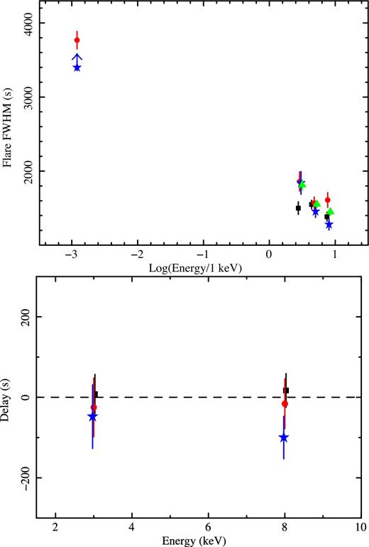
(Top panel) Flare duration (FWHM) at various energies of the three brightest XMM–Newton flares, VB1, VB2, VB3 and of the combined XMM–Newton flare light curve are shown with back squares, red circles, blue stars and green triangles, respectively. The flare duration are computed in the 2–4, 4–6 and 6–10 keV energy bands (the points are slightly shifted for display purposes). Flares are typically shorter at higher energies. We also show the duration of VB2 (as observed in the L band, see Section 5.2) and the lower limit on the duration of VB3 (as observed with SINFONI). The flare durations in the NIR band connect with the extension of the trend observed in X-rays. (Bottom panel) Peak occurrence delay, between different energies (same energy bands as above) for the three very bright flares observed by XMM–Newton. The delays are computed as the best-fitting peak value of the Gaussian at each energy minus the same value observed in the 4–6 keV band. Colour code as before.
The top panel of Fig. 11 suggests that Sgr A*'s flares shorten with energy, typically lasting ∼5 per cent less time in the hard band (6–10 keV) compared to the soft one (2–4 keV). The top panel of Fig. 12 shows the combination of all three very bright flares. With the solid red, dotted orange and dashed blue lines the light curves in the 2–4, 4–6 and 6–10 keV energy bands are shown. The light curves are shifted by the centre of their best-fitting Gaussian profile, subtracted by the best-fitting local underlying continuum, and normalized by the peak of their best-fitting Gaussian (see Table 7). The flare profile is tighter at higher energies (Fig. 12, Table 7). Indeed, the width of the Gaussian fitting the 6–10 keV band appears to be significantly smaller (at ∼4.4σ significance) by ∼360 s compared to the 2–4 keV band one (see Table 7). To test whether this is a common property of all X-ray flares or whether it is a peculiarity of very bright flares, we combined all Chandra bright and very bright flares (i.e. with fluence larger than 5 × 10⁻⁹ erg cm−2; see Ponti et al. 2015c for the definition). To avoid flares significantly affected by pile up, we excluded the ones observed in either ACIS-I or ACIS-S with no subarray mode and reaching a block count rate equal or higher than 0.1 ph s−1 (see Ponti et al. 2015c for details). We also excluded the flares observed in ACIS-S 1/8 subarray mode and reaching a block count rate equal or higher than 0.8 ph s−1 (Ponti et al. 2015c). The bottom panel of Fig. 12 shows the combined Chandra flare light curve in the 2–4.5 and 6–9 keV energy bands with red circles and blue squares, respectively. We find that bright Chandra flares also last longer in the soft energy band compared to the hard one, with a difference in FWHM of ∼300 s (Fig. 12 and Table 7).
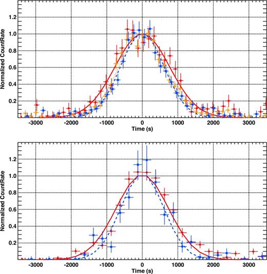
(Upper panel) The combination of the light curves of VB1, VB2 and VB3 in the 2–4 keV (red squares), 4–6 keV (orange stars), 6–10 keV (blue squares), light curves are shifted by the centre of their best-fitting Gaussian profile, subtracted by the best-fitting local underlying continuum, and normalized by the peak of their best-fitting Gaussian. Time bins of 150 s are used. Flares are shorter in the hard band. (Bottom panel) Chandra composite light curve for 2–4.5 keV (red circles) and 6–9 keV (blue squares). All bright flares not significantly affected by pile-up (peak count rate <0.1 ph s−1) are considered here. The light curves are shifted with the same method described above. Time bins of 250 s are used. Flares last longer in the soft band.
Results of single Gaussian fitting to the 200 s binned flare light curves without background subtraction, but with epiclccorr applied. Note that using the background subtracted light curves only changes these values very slightly. abThe errors are all 1σ. The composite flare from XMM–Newton is the combination of VB1, VB2 and VB3. The composite flare from Chandra is the combination of a set of unpiled-up flares observed by Chandra.
| Flare ID | Band | Continuuma | FWHM | Delayb |
|---|---|---|---|---|
| (keV) | (cts s−1) | (s) | (s) | |
| VB1 | 2–4 | 0.0446 ± 0.0017 | 1500 ± 85 | +8 ± 49 |
| 4–6 | 0.0310 ± 0.0014 | 1550 ± 57 | 0 | |
| 6–10 | 0.0128 ± 0.0009 | 1385 ± 61 | +17 ± 42 | |
| VB2 | 2–4 | 0.0485 ± 0.0008 | 1860 ± 130 | −25 ± 73 |
| 4–6 | 0.0433 ± 0.0008 | 1570 ± 80 | 0 | |
| 6–10 | 0.0198 ± 0.0005 | 1610 ± 100 | −16 ± 62 | |
| VB3 | 2–4 | 0.0956 ± 0.0016 | 1840 ± 153 | −48 ± 79 |
| 4–6 | 0.0893 ± 0.0015 | 1455 ± 80 | 0 | |
| 6–10 | 0.0273 ± 0.0008 | 1280 ± 75 | −100 ± 53 | |
| Composite | 2–4 | 0.0610 ± 0.0007 | 1813 ± 68 | – |
| (XMM) | 4–6 | 0.0559 ± 0.0007 | 1554 ± 42 | – |
| 6–10 | 0.0242 ± 0.0004 | 1450 ± 47 | – | |
| Composite | 2–4.5 | 7.9 ± 0.3 × 10⁻⁴ | 1730 ± 56 | – |
| (Chandra) | 4.5–6 | 4.1 ± 0.2 × 10⁻⁴ | 1693 ± 59 | – |
| 6–9 | 6.0 ± 0.4 × 10⁻⁴ | 1424 ± 89 | – |
aBest-fitting local continuum under the flare.
bDelay time related to the 4–6 keV band.
No significant time shift with energy is apparent, with upper limits as tight as ∼100–200 s (see bottom panel of Fig. 11).
We conclude that, at present, the X-ray data of the bright flares are not in contradiction with a slow variation of γmax.
8 DISCUSSION
Simultaneous XMM–Newton, NuSTAR and SINFONI observations of Sgr A* allowed us to determine, for the first time, the spectral shape and the evolution of the radiation of a very bright flare. This enabled us to pin down the radiative mechanism during bright flares of Sgr A* and its evolution during the flare. We can rule out that a simple power-law model, representing plain synchrotron emission, can reproduce the flare emission.
8.1 TSSC
A TSSC model provides an acceptable fit to the data, from a statistical point of view. However: (i) the fit is worse than the PLCool and PLCoolEv models, despite the larger number of free parameters; (ii) in this framework the observed spectral steepening (ΔΓ = 0.57 ± 0.09 at 1σ) between NIR and X-ray would be just a coincidence, moreover; (iii) the best-fitting parameters appear implausible.
Indeed, the best-fitting magnetic field appears unreasonably high (B ∼ 104), the source size unphysically small (RF ∼ 10−2 to 10−4RS) and the required source density about seven orders of magnitude higher than what is estimated to be present in the accretion flow around Sgr A* (Loeb & Waxman 2007; Genzel et al. 2010). As discussed in Dodds-Eden et al. (2009), these unreasonable best-fitting parameters are consequences of the assumptions intrinsic to the TSSC model considered here. In particular, to fit the soft X-ray emission via inverse Compton up-scattering of NIR or sub-mm radiation, the energies of the electrons involved in the flare is restricted to be lower than γe < 100. On the other hand, the requirement of the observed hard NIR slope constrains the magnetic field to be larger than B > 103 G. Finally, the ratio of the synchrotron to inverse Compton luminosity requires that the size of the source has to be RF < 10−2RS. Therefore, it appears that this simplistic TSSC model, cannot adequately explain the flare emission.
The observed spectral steepening (ΔΓ = 0.57 ± 0.09, 1σ) between NIR and X-rays of the mean spectrum suggests that the radiative process during bright flares might be synchrotron radiation with a cooling break. Therefore, we explored in more details this scenario, instead of considering more complex synchrotron self-Compton (SSC) models. Nonetheless, this does not rule out that more complex TSSC and non-thermal SSC models might be invoked to explain the X-ray radiation.
8.2 PLCool
We observed that the synchrotron model with a cooling break can reproduce both the mean spectrum and the evolution of the SED of Sgr A* during the entire duration of a very bright flare (apart from IR2). In particular, the observed spectral steepening of both the mean spectrum and of the emission at the X-ray peak (IR3) is a strong indication that synchrotron with cooling break might be the dominant radiative mechanism. In this simplistic model, the ‘unknown’ motor powers the continuous acceleration of energetic electrons with a power-law distribution. An important difference of the PLCool model compared to the TSSC model is that the motor is assumed to accelerate electrons into a power-law distribution up to γmax ≥ 106; therefore, the synchrotron radiation is not limited to the NIR band, instead it extends to X-ray and higher energies.
8.2.1 Limitations of the model
We point out that, for simplicity, we reproduce the synchrotron emission with a simple BPL model. We note that the cooling break typically occurs in the unobserved optical–UV band; therefore, we cannot currently constrain whether the cooling break is a sharp feature or it is significantly extended in energy. Indeed, we do not observe any significant curvature in either the NIR or X-ray band; however, this has to be attributed to the small frequency windows sampled by our data. Therefore, for simplicity, we assume a sharp break, though realistic synchrotron models can be significantly broadened (by up to more than a decade in energy; Dibi et al. 2014). Indeed, it is beyond the scope of this paper to employ more complex synchrotron models. We also note that significantly different statistics characterize the time-resolved spectra in the NIR and X-ray bands. Therefore, the broad-band fit of the time-resolved spectra are primarily driven by the NIR photon index. It is important to point out that at the beginning of the flare, the cooling break is observed to be located either within or very close to the NIR band. Therefore, should a broadened break be present at that time, it might potentially affect some of the model parameters. Future investigations will clarify the extent of this.
8.2.2 Difficulties of the PLCool model
As already briefly mentioned in Section 5.6, we stress again here that the most difficult problem of the PLCool model is related to the best-fitting energy of the cooling break. Indeed, both for IR1 and IR2 the break is observed within the NIR band (see Table 6). During IR1 this result is driven by the combined upper limit on the X-ray emission and by the high flux and flat photon index in the SINFONI band, inducing a cooling break suspiciously located at energies just higher than ∼0.6 eV, the upper bound of the SINFONI spectrum. Similar results hold during IR2. Indeed, at that time, the X-ray flare had already started, alleviating the problem, however the NIR band showed a slightly flatter power law (ΓNIR = 1.59 ± 0.2; Table 3); therefore, the cooling break was observed to again be placed at the upper bound of the SINFONI spectrum (moreover the steep X-ray slope is not completely reproduced). We consider a rather unlikely possibility that, by chance, the cooling break occurred twice within the narrow NIR band.
The biggest pitfall that the PLCool model has to overcome is the explanation of the early phases of the VB3 flare. Indeed, at the basis of the PLCool model there is the assumption that the NIR and X-ray emissions are tied by a BPL. Therefore, within this framework one would predict that the NIR to X-ray emission are strictly related and they follow each other. The only deviation to this ‘rule’ could be generated by the possible delay of the NIR radiation associated with the longer NIR synchrotron cooling time. Therefore, it is expected that the X-ray emission either rises before or at the same time as the NIR one. One possible way out (that has been considered in the past to explain the delayed X-ray emission in the early phases of the very bright flares) was to assume that the early NIR emission had a very steep slope. However, we can now rule out that this is happening during VB3. Indeed, during IR1 bright NIR emission, with a flat slope (ΓNIR = 1.48 ± 0.2; Table 3), is observed at the same time of tight upper limits to the X-ray emission. On the contrary, no prominent X-ray radiation is observed either during or before IR1, with upper limits in the 3–10 keV band of F3–10keV < 2.3 × 10⁻¹² erg cm−2 s−1.
The third difficulty of the PLCool model is to properly reproduce the IR2 spectrum. A fit with the BPL model shows that the difference of the X-ray to NIR photon index is significantly higher ΔΓ = 1.8 ± 0.4 than the one expected by the cooling break model ΔΓ = 0.5 (Table 6). This resulted in a poor fit of IR2 by the PLCool model (indeed an F-test suggests that the BPL model provided a significantly better description of the IR2 spectrum, at >99 per cent confidence).
8.3 PlCoolEv
We then relaxed the requirement that γmax has to be >106 at all times. We postulated that, γmax increases slowly with time (e.g. many times the Alfvén speed crossing time of a source of a size of few Schwarzschild radii), generating a cut-off that gradually moves to higher energies, eventually transiting through the X-ray band and producing a bright X-ray radiation with a delay compared to the start of the NIR flare. Regardless of the behaviour of γmax at the end of the flare, the PLCoolEv (as well as PLCool) model predicts a delay of a few hundred seconds of the NIR radiation, compared to the X-ray emission (Section 5.8), in agreement with a longer duration of the NIR flare.
8.3.1 Limitations of the model
For simplicity, we assumed an exponential drop of the high-energy cut-off in the synchrotron spectrum, with a shape such that the e-folding energy is equal to the cut-off energy. We note that the high-energy cut-off is detected in the observed band only once, during IR2. During this interval, the X-ray slope is steeper (Γ = 3.2 ± 0.4) than the simultaneous NIR one; however, the statistics is not enough to discriminate its detailed shape. For example, we could not distinguish either between an exponential or a sub-exponential, or we could not constrain the broadness of the cut-off. Therefore, should a broadened break be present at that time, it might potentially affect some of the model parameters. For instance, broader cut-offs in IR2 and IR4 might allow for a cooling break at higher energy, implying a weaker magnetic field. Future investigations will clarify the extent of this.
8.3.2 Comparison of the PLCoolEv model to the data
The PLCoolEv model provides an excellent description of the mean spectrum of VB3 and of its evolution over time. In fact, it naturally explains the periods during which bright and flat-spectrum NIR radiation is observed, simultaneous with no X-ray emission (e.g. IR1). In particular, the passage of the cut-off within the X-ray band generates: (i) shorter flare durations at higher energies; (ii) right at the start of the X-ray flare steeper X-ray spectra than expected by the cooling break (e.g. IR2) and (iii) possibly steeper spectra in the flanks of the X-ray flare than at the peak, such as observed.
We also measured a significant evolution of the cooling break during the flare. Under the assumption that the escape time remains constant, this suggests that the strength of the magnetic field (typically of several tens of Gauss) lowers to values of few Gauss during the peak of bright flares, to return to high values after that. For a thermal distribution of electrons with temperature θE, the synchrotron luminosity is proportional to the square of the magnetic field (|$L_{\text{Synch}}\propto N\theta ^2_{\rm E} B^2$|); therefore, the drop of the magnetic field strength at the flare peak would appear contradictory. However, in this scenario, the large synchrotron luminosity is provided by the vast increase in the energy of the accelerated particles. It is likely that the acceleration mechanism is powered by the magnetic field that therefore gradually reduces its strength during the flare (Dodds-Eden et al. 2009, 2010, 2011). Indeed, a similar process is at work in magnetic reconnection that is a fundamental process of plasmas in which magnetic energy is converted into particle acceleration through magnetic field rearrangement and relaxation (Begelman 1998; Lyubarsky 2005; Zweibel & Yamada 2009; Sironi & Spitkovsky 2014; Sironi, Giannios & Petropoulou 2016). The observed drop of the magnetic field, right at the peak of the flare, is in line with the predictions of magnetic reconnection models.
We conclude that the data are consistent with such an evolution of the magnetic field.
8.3.3 Constraints on energy power and source size
Is the energy stored in the magnetic field enough to power the flare? We estimated the total energy emitted during the VB3 flare by considering that the NIR and X-ray luminosity was at a level of ∼10 mJy and ∼2 × 1035 erg s−1 for about ∼3.8 × 10³ and ∼1.8 × 10³ s, respectively, resulting in a total emitted energy of ∼8 × 1038 erg. If we discharge the magnetic energy within a spherical region with ∼1.5RS radius, bringing its magnetic field from B ∼ 30–40 to ∼5 G, then about ∼8–15 × 1038 erg are produced. This appears to be enough energy to power the VB3 flare. Moreover, this suggests that the source of VB3 had a size ≥1.5RS.
9 CONCLUSIONS
The mean X-ray photon index during the very bright flare VB3 is significantly steeper (ΓX = 2.27 ± 0.12) than the simultaneous (ΓNIR = 1.7 ± 0.1) NIR one, excluding that the radiative process can be described by a simple power law. In particular, the observed steepening (ΔΓ = 0.57 ± 0.09 at 1σ) is consistent with what is expected by synchrotron emission with a cooling break (ΔΓ = 0.5).
We observe bright F2.2μm = 8.9 ± 0.1 mJy and hard NIR (ΓNIR = 1.48 ± 0.23) emission about ∼103 s before the start of the X-ray flare. We also observe very steep X-ray emission (ΓX = 3.2 ± 0.4) at the start of the X-ray flare, while the contemporaneous NIR photon index was ΓNIR = 1.4 ± 0.2. These results strongly support a scenario where the synchrotron emitting electron power-law distribution has a cut-off (γmax) that is slowly evolving with time, therefore inducing an evolving high-energy cut-off in the spectrum.
The data are consistent with an evolution of the magnetic field strength during the flare (under the assumption of a constant escape time). Large magnetic field amplitudes (B = 30 ± 8 G) are observed at the start of the X-ray flare. The magnetic field strength drops to B = 4.8 ± 1.7 G, at the peak of the X-ray flare, a variation of a factor of >6 in less than ∼650 s. It then increases again in the decreasing flank of the flare (|$B=14.3^{+12.3}_{-7.0}$| G). This is consistent with a scenario where the process that accelerates the electrons producing the synchrotron emission is tapping energy from the magnetic field (such as, e.g. in magnetic reconnection).
From the total emitted energy and the variation of the magnetic field, we estimated that the source size of the VB3 flare has to be larger than ≥1.5RS, if powered by magnetic reconnection.
We observe hints for steeper, by roughly ΔΓ = 0.3, X-ray spectra during the rise and the decay of an X-ray flare, compared to the values at peak. This indicates that, despite the fact that the photon index is similar between different X-ray flares, there might be significant spectral evolution during each X-ray flare. This is an expectation of the PLCoolEv model.
Bright and very bright XMM–Newton and Chandra flares typically last significantly (∼4.4σ significance) longer, by ∼300 s at soft X-ray energies, compared to harder ones (2–4 and 6–10 keV, respectively). This trend appears to join smoothly to the longer duration typically observed in the NIR band. Again, this is most probably the product of the evolution of γmax.
The three very bright flares, caught by XMM–Newton so far, have very similar light curves and spectral properties, indicating an analogous physical origin. This suggests that the results of this study on VB3 could be universal to bright and very bright flares.
The best-fitting column density of neutral absorbing material observed during the X-ray spectra of the very bright flares of Sgr A* is constant and it is consistent with the values observed in nearby sources. Indeed, the three bright transients within dpro < 1.5 arcmin from Sgr A* (SGR J1745−2900, Swift J174540.7−290015 and the foreground component towards AX J1745.6−2901) show neutral absorption column densities consistent with the value of Sgr A* (Coti-Zelati et al. 2015; Ponti et al. 2016a,b). This suggests that the neutral absorption towards Sgr A* has an ISM origin.
Synchrotron self-Compton models can statistically reproduce the flare emission and its evolution. On the other hand, they imply unrealistic parameters. In such a scenario it would be an unlikely coincidence that the NIR photon index is flatter than the X-ray one by ΔΓ = 0.5. Moreover, the evolution of the density, source radius and magnetic field before, during and after the very bright flare appears improbable.
Acknowledgments
The authors wish to thank Jan-Uwe Ness, Ignacio de la Calle, Karl Foster and the rest of the XMM–Newton and NuSTAR scheduling teams for the enormous support that made this multiwavelength campaign possible, as well as the referee for the careful reading of the paper. GP thanks Mark R. Morris, Gabriele Ghisellini, Lorenzo Sironi, Hendrik J. van Eerten, Michi Bauböck and Francesco Coti-Zelati, for useful discussion. RT and AG acknowledge support from CNES. This research has made use both of data obtained with XMM–Newton, an ESA science mission with instruments and contributions directly funded by ESA Member States and NASA, and on data obtained from the Chandra Data Archive. The GC XMM–Newton monitoring project is supported by the Bundesministerium für Wirtschaft und Technologie/Deutsches Zentrum für Luft- und Raumfahrt (BMWI/DLR, FKZ 50 OR 1408 and FKZ 50 OR 1604) and the Max Planck Society.
RS is the Schwarzschild radius RS = 2GMBH/c2, where MBH is the BH mass, G the gravitational constant and c the speed of light.
Interestingly, AGN of similar BH mass, but clearly much higher accretion rate, shows power-density spectra (PDS) of their X-ray light curves consistent with the NIR PDS of Sgr A* (Meyer et al. 2009).
Indeed, the few multiwavelength campaigns that caught a very bright X-ray flare were missing spectroscopic information in the NIR band (e.g. Dodds-Eden et al. 2009), while the few campaigns with spectroscopic information in both bands, failed to detect a bright X-ray flare with an NIR counterpart (e.g. flare A and B of Trap et al. 2011).
XMM–Newton User Handbook, Issue 2.14, 2016 (ESA: XMM-Newton SOC), Longinotti et al. (2014).
The large uncertainty in this measurement is driven by the uncertainty in the determination of the fraction of column density in the foreground component.
The authors find marginal evidence for sub-Solar iron abundance, suggesting that iron is depleted into dust grains. The detailed investigation of the metal abundances is beyond the scope of this paper.
The normalizations are, however, consistent between the two instruments.
Defined on the basis of the X-ray light curve; therefore, it represents the full duration of the X-ray flare.
The fits have been performed in matlab, implementing the equations reported in Dodds-Eden et al. (2009) and references therein. The best fit was computed through a χ2 minimization technique. The parameter space to determine the uncertainties on the best-fitting parameters has been explored through a Bayesian Markov Chain Monte Carlo approach.
An excessively compact source with such high densities and magnetic field is hardly achievable event through compression of a fraction of the quiescent electrons. The quiescent density of electrons (ne = 106 cm−3) dictates that Ne = 1039.5 electrons are contained within a sphere of ∼0.07RS, that therefore would need to be compressed by 2.3 orders of magnitude to reach the required TSSC source size and density. We note that, assuming conservation of the magnetic flux, the magnetic field strength would rise to log(B) ∼ 6.2, two orders of magnitude higher than the best-fitting value. The magnetic energy would also rise, but would still be 2–4 orders of magnitude smaller than the one required to power the flare.
Synchrotron radiation from the cooling power-law distribution of electrons (with electron power-law index p) generates a spectrum νFν ∝ ν(3 − p)/2 at frequencies lower than the cooling break and νFν ∝ ν(2 − p)/2 above. This implies that p relates to the photon index Γ such as: |$\Gamma =\frac{p+1}{2}$| below and |$\Gamma =\frac{p+2}{2}$| at frequencies above the cooling break.
More observations are needed to confirm the tentative hint for a steeper NIR slope in the early phase of the NIR flare (IR1 and IR2 compared to IR3 and IR4; see Table 6).
Assuming that all emission is radiated at 0.29 times the critical frequency, it follows that: νc ∼ 2.5 × 10¹⁹ Hz (γmax/106)2 (B/20 G) (Longair 2011, equation 8.127), where νc is the frequency associated to the high-energy cut-off.
Would, during IR4, the cut-off be located in the X-ray band or below, then the current constraints on the energy of the cooling break should be considered only as upper limits. If this is indeed the case during IR4, then weaker magnetic fields would be allowed and the data point in Fig. 9 should be considered as an upper limit.
We do not consider bright flares detected by Chandra, because the vast majority of those are affected by strong pile-up, significantly distorting the spectral shape.
The variation of the non-flare emission during both observations taken on 2007 April 3 and 2014 August 31 was produced by the contribution from the magnetar SGR J1745−2900 (at the level of ∼50 per cent to the total observed quiescent flux on 2014 August 30; see also Ponti et al. 2015c) and from the very bright source AX J1745.6−2901 (Ponti et al. 2015a).
REFERENCES
APPENDIX A: FURTHER DETAILS ON XMM–NEWTON DATA REDUCTION
All X-ray observations considered here have been accumulated with the EPIC-pn and EPIC-MOS cameras in Full Frame mode with the medium filter applied (apart from obsID 0111350301 which has the pn camera with the thick filter; see Ponti et al. 2015a,b). Sgr A*'s flares in Table 1 occurred during periods of negligible soft proton flare activity; therefore, no cut was performed during those flares. On the other hand, significant soft proton flares are detected during quiescent emission. We removed these periods of enhanced background activity by cutting all intervals with more than 0.25 ph s−1 in the background light curve (integrated over the 10–15 keV energy band, with 20 s time bins and extracted from a 3 arcmin radius). We selected only single and double events and we used (FLAG == 0) and either (#XMMEA_EP) or (#XMMEA_EM) for EPIC-pn or EPIC-MOS, respectively. We applied the sas task LCCORR to the XMM–Newton light curves.
We note that during obsID: 0743630201, 0743630301 and 0743630501 Sgr A*'s flux is contaminated by the X-ray emission from the magnetar SGR J1745−2900, located at only ∼2.4 arcsec from Sgr A* (Degenaar et al. 2013; Mori et al. 2013; Rea et al. 2013). During these observations the magnetar's flux was F1-10keV ∼ 3 × 10⁻¹² erg cm−2 s−1 (see Coti Zelati et al. 2015; for the details of the decay curve), therefore allowing an adequate characterization of the bright flares.
‡ We report in Table 1 the same time systems as used by XMM–Newton (see section 6.1.4 in XMM–Newton Users Handbook, https:heasarc.gsfc.nasa.govdocsxmmuhbreftime.html). The reference or zero time has been defined as: 1998-01-01T00:00:00.00 TT = 1997-12-31T23:58:56.816 UTC. The conversion from TT to UTC at the reference date is TT = UTC + 63.184 s and can be derived from The Astronomical Almanac for other dates.
APPENDIX B: SPECTRAL DISTORTIONS INTRODUCED BY DUST SCATTERING
As already discussed in Section 3.1, dust scattering does severely distort the source spectrum and if its effects are not properly taken into account, it could significantly bias the results. To provide the reader with a better understanding of the extent of this effect on the various best-fitting parameters, we present in Table B1 the best-fitting results of the mean X-ray spectrum of VB3 after the application of: (i) no correction; (ii) corrections with the dust model and (iii) correction with the fgcdust model. For these fits, we left the column density of neutral absorbing material free to vary. When we applied the dust model, we tied the dust scattering optical depth τ to the fitted column density so that τ = 0.324(NH/1022 cm−2), following Nowak et al. (2012). We also assumed a ratio of 10 between the size of the halo at 1 keV and the extraction region.
Best-fitting parameters, once the mean X-ray spectrum of VB3 is corrected with different dust scattering models. Column densities are in 1023 cm−2 units. Fluxes are in 10−12 erg s−1 cm−2 units, integrated over the 3–10 keV band and are absorbed, but corrected for the effect of dust scattering. The XMM–Newton spectrum is fitted with an absorbed power law modified by the dust scattering.
| No dust | dust | fgcdust | |
|---|---|---|---|
| NH | 1.8 ± 0.3 | 1.3 ± 0.2 | 1.6 ± 0.3 |
| Γ | 2.0 ± 0.3 | 2.1 ± 0.3 | 2.2 ± 0.3 |
| F3–10 | |$7.4^{+10.8}_{-3.6}$| | |$8.3^{+7.2}_{-3.7}$| | |$8.9^{+9.0}_{-4.4}$| |
| χ2/dof | 125.8/116 | 124.2/116 | 126.9/116 |
| No dust | dust | fgcdust | |
|---|---|---|---|
| NH | 1.8 ± 0.3 | 1.3 ± 0.2 | 1.6 ± 0.3 |
| Γ | 2.0 ± 0.3 | 2.1 ± 0.3 | 2.2 ± 0.3 |
| F3–10 | |$7.4^{+10.8}_{-3.6}$| | |$8.3^{+7.2}_{-3.7}$| | |$8.9^{+9.0}_{-4.4}$| |
| χ2/dof | 125.8/116 | 124.2/116 | 126.9/116 |
The best-fitting results in Table B1 show that the inclusion of the dust scattering model allows us to recover a steeper and brighter source spectrum. Indeed, the main effect of dust scattering is to remove flux from the line of sight and to spread it in the halo, which is typically partly lost because of the small source extraction region. Moreover, the probability of dust scattering is higher at low energy, producing a deficiency of low-energy photons in the observed spectrum (that is generally reproduced by a higher column density of absorbing material and flatter spectra). Therefore, once the correction for dust scattering is introduced, we observe that the flux increases by ∼20 per cent, the column density of neutral material is lower and the spectrum steepens. In particular, we observe the photon index to steepen by ΔΓ ∼ 0.2. It is important to note that different dust models lead to photon indexes that differ by ΔΓ = 0.1 (see Table B1).
For this reason, we performed again all the analyses in the paper, correcting the effects of dust scattering with the dust model. The fit of the mean VB3 X-ray spectrum results in a ΓX = 2.16 ± 0.14, that once compared to the NIR slope ΓNIR = 1.7 ± 0.1, gives ΔΓ = 0.46 ± 0.17 (±0.10 at 1σ), which is completely consistent with the PLCool model (ΔΓ = 0.5). The same applies also to the IR3 interval. Indeed, the X-ray photon index during IR3 is ΓX = 2.5 ± 0.3, therefore steeper by ΔΓ = 0.6 ± 0.3, compared to the simultaneous NIR measurement (|$\Gamma _{\text{NIR}}=1.9^{+0.1}_{-0.2}$|). Therefore, it is in this case also consistent with the conclusions of this work.
The blue, green, and black data in Fig. B1 show the XMM–Newton de-absorbed mean spectrum of VB3 (see also Fig. 4) after correcting the observed spectrum for the effects of dust scattering with the fgcdust, dust models and after applying no correction, respectively. The blue dotted lines show the uncertainties in the determination of the X-ray slope if no correction for dust scattering is applied. Even in this case, the difference in X-ray and NIR spectral shapes are consistent with the predictions of the synchrotron model with cooling break.
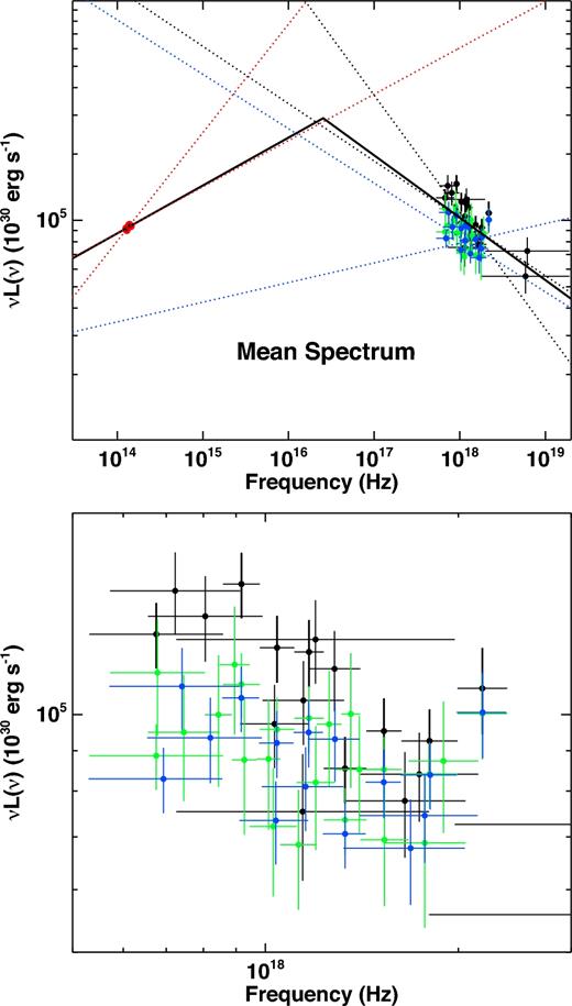
(Top panel) The red points show the mean NIR (SINFONI) during the VB3 flare, such as in Fig. 4. The blue points show the corresponding X-ray (XMM–Newton and NuSTAR) spectra, when no dust correction is applied. The green and black points show the X-ray spectra corrected for the effects of dust scattering according to the dust and fgcdust models, respectively. The stronger the correction, the brighter and steeper becomes the X-ray spectrum (see text for details). The red, blue and black dotted lines show the uncertainty on the NIR slope, on the X-ray slope when no correction for dust is applied and once the data are corrected using the fcgdust model, respectively. The black line shows the best-fitting PLCool model (where the X-ray and NIR slopes are tied). All data and models and data are de-absorbed. (Bottom panel) Enlargement of the top panel into the X-ray band, to allow a better elucidation of the extent of the effect.
